Article

Theoretical Analysis of a Fractional-Order LLCL Filter for Grid-Tied Inverters

1
School of Mechanical and Electrical Engineering, Guangzhou University, Guangzhou 510006, China
2
School of Electronics and Communication Engineering, Guangzhou University, Guangzhou 510006, China
*
Author to whom correspondence should be addressed.
Fractal Fract. 2023, 7(2), 135; https://doi.org/10.3390/fractalfract7020135
Submission received: 9 January 2023 / Revised: 25 January 2023 / Accepted: 29 January 2023 / Published: 31 January 2023

Abstract

:
The LLCL-filter-based grid-tied inverter performs better than the LCL-type grid-tied inverter due to its outstanding switching-frequency current harmonic elimination capability, but the positive resonance peak must be suppressed by passive or active damping methods. This paper proposes a class of fractional-order LLCL (FOLLCL) filters, which provides rich features by adjusting the orders of three inductors and one capacitor of the filter. Detailed analyses are performed to reveal the frequency characteristics of the FOLLCL filter; the orders must be selected reasonably to damp the positive resonance peak while reserving the negative resonance peak to attenuate the switching-frequency harmonics. Furthermore, the control system of the grid-tied inverter based on the FOLLCL filter is studied. When the positive resonance is suppressed by the intrinsic damping effect of the FOLLCL filter, the passive or active damper can be avoided; the grid current single close-loop is adequate to control the grid-tied inverter. For low-frequency applications, proportional-resonant (PR) controller is more suitable for the FOLLCL-type grid-tied inverter compared with the proportional-integral (PI) and fractional-order PI controllers due to its overall performance. Simulation results are consistent with theoretical expectations.

1. Introduction

The grid-tied inverter is widely used in renewable energy generation; the voltage-source inverter (VSI) interfaces with the grid through a low-pass filter to limit the excessive current harmonics. A third-order LCL filter is the most popular solution over a first-order L filter due to its smaller size, lower cost, and better harmonic attenuation capability [1,2,3,4,5]. However, large inductance should be selected for an LCL filter in low-frequency applications to suppress the more abundant current harmonics. To solve this problem, a high-order LLCL filter has been proposed in [6] and further developed in [7,8,9,10,11,12,13,14,15]. Based on the LCL filter, a small inductor is inserted in series with the capacitor to form a series resonant branch. The series resonant frequency is thus designed to further attenuate the switching harmonics. The total harmonic distortion (THD) of the grid current will be much lower with LLCL-type inverters compared with LCL-type ones in low-frequency applications.
However, the LLCL filter retains the positive resonant feature of the LCL filter, which causes system instability. Passive or active dampers are used to mitigate the impact of the positive resonance, leading to power loss or control complexity. It is even worse that the capacitor current feedback, the most commonly used active damping method, may introduce a negative resistance and cause instability due to the control delay [8].
In recent years, the fractional-order modeling of power converters has been paid much attention because the inductors and capacitors, the key components of power converters, have fractional-order characteristics, or can be specially designed as fractional-order components. The research of fractional-order power converters began from the modeling of DC–DC converters. In [16], fractional calculus and the circuit-averaging technique are used to model the buck converter. This technique is also used to build the model of the fractional-order magnetic coupled boost converter [17]. The fractional-order model of the buck converter based on the Caputo–Fabrizio derivative is presented in [18]. The Riemann–Liouville derivative is also used to obtain more accurate models of the fractional-order buck converter [19] and fractional-order buck–boost converter [20]. Instead of considering the complex definitions of fractional calculus, the harmonic balance principle and equivalent small parameter method are used to describe the fractional-order DC–DC converters [21]. Different from the above studies, time domain expressions for fractional-order DC–DC converters are derived in [22]. The modeling methods for fractional-order DC–AC converters are also reported in the literature. In [23], the Caputo derivative method is used to build the model of the voltage source converter, and small-signal analysis and averaging state-space model-based analysis are developed. The fractional-order model of the three-phase voltage source PWM rectifier is constructed in [24]; the Caputo fractional calculus operator is used to describe the fractional-order characteristics of the inductor and capacitor. In addition, the influence of the orders of the inductors and the capacitor on the operating characteristics of the PWM rectifier is studied. In [25], an LCαL filter-based grid-connected inverter is modeled and a filter design example is given. However, the above literature only focuses on the modeling methods; the control strategies are not considered.
On the other hand, fractional-control theories are developed to control the power converters. The fractional-order PID control method is employed to regulate DC–DC converters [26,27]; the results show that the method achieves less overshoot and a faster recovery time compared to the integer-order PID regulator. In [28], the factional-order adaptive sliding mode control approach is proposed for fractional-order buck–boost converters, which shows stronger robustness under various disturbances. For LCL-type grid-tied inverters, an active damping method based on fractional-order proportional-derivative (PD) grid current feedback is presented in [29], which shows better performance compared to the integer-order PD damping method. In [30], a capacitive current fractional proportional-integral feedback strategy is proposed to increase the limit of the damping region of the LCL grid-tied inverter under the weak grid condition. A fractional-order LCL (FOLCL) filter-based grid-tied inverter is studied in [31]; the capacitor current feedback loop can be omitted by only changing the orders of the passive components. Especially, PI and fractional-order PI controllers especially are designed for this grid-tied inverter.
Considering the advantages of fractional-order converters, this paper proposes a fractional-order LLCL-type grid-tied inverter, which can avoid the use of an active damper. The contributions of this paper include the following points:
  • The characteristics of the FOLLCL filter is analyzed, including the condition of resonance, magnitude–frequency characteristic, phase–frequency characteristic, and the impacts of inductor and capacitor orders on the characteristics.
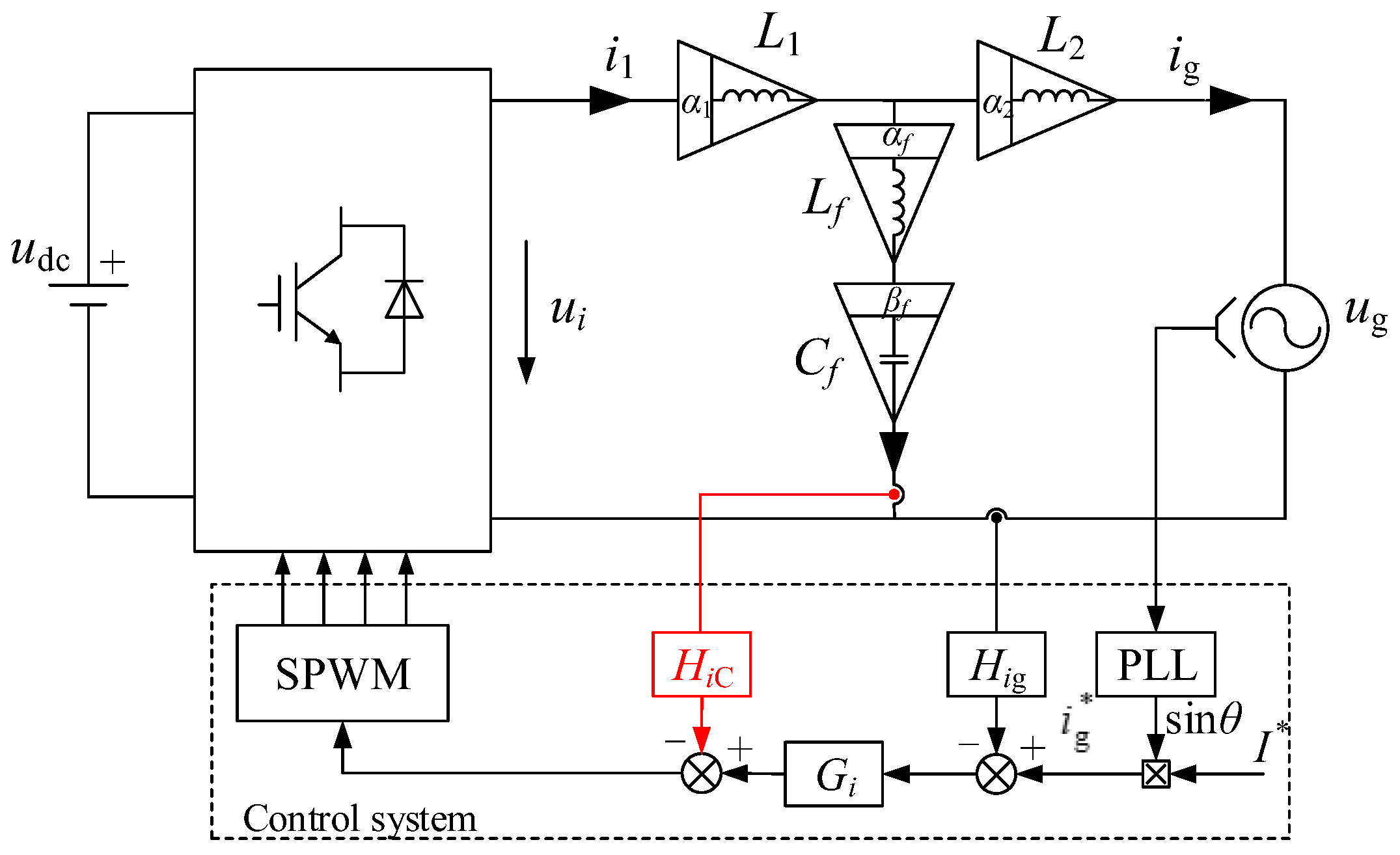
  • The control system of the FOLLCL-type grid-tied inverter is given. Active damping can be avoided, thus improving the ease of control and saving the cost of the control system.
  • The performances of the FOLLCL-type grid-tied inverter based on PI, PIλ, and PR control are analyzed through four cases. Among these three control methods, the most suitable one for the FOLLCL-type grid-tied inverter without an active damper is determined.
The remainder of the paper is organized as follows: Section 2 introduces the integer-order LLCL (IOLLCL) filter and makes a comparison between the IOLLCL filter and the IOLCL filter. Section 3 analyzes the characteristics of the FOLLCL filter, including resonant frequency, magnitude–frequency characteristic, and phase–frequency characteristic. In Section 4, the structure of the control system of the FOLLCL-type grid-tied inverter is described. Based on the expression of loop gain, the system performance is analyzed. Four cases are presented to discuss the performance of the FOLLCL-type grid-tied inverter. The simulation results are given in Section 5 to validate the theoretical analysis. Finally, Section 6 concludes this paper.

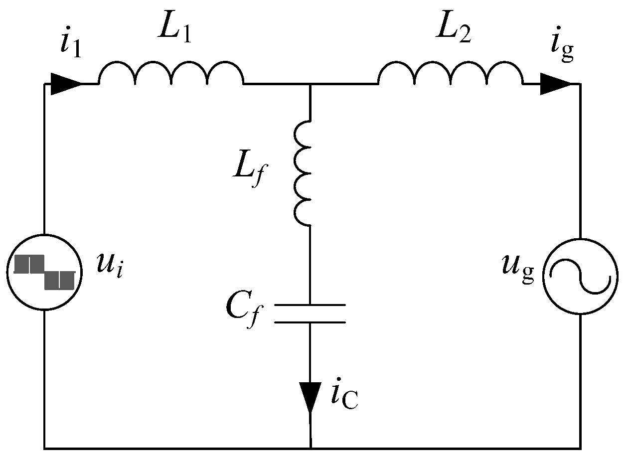
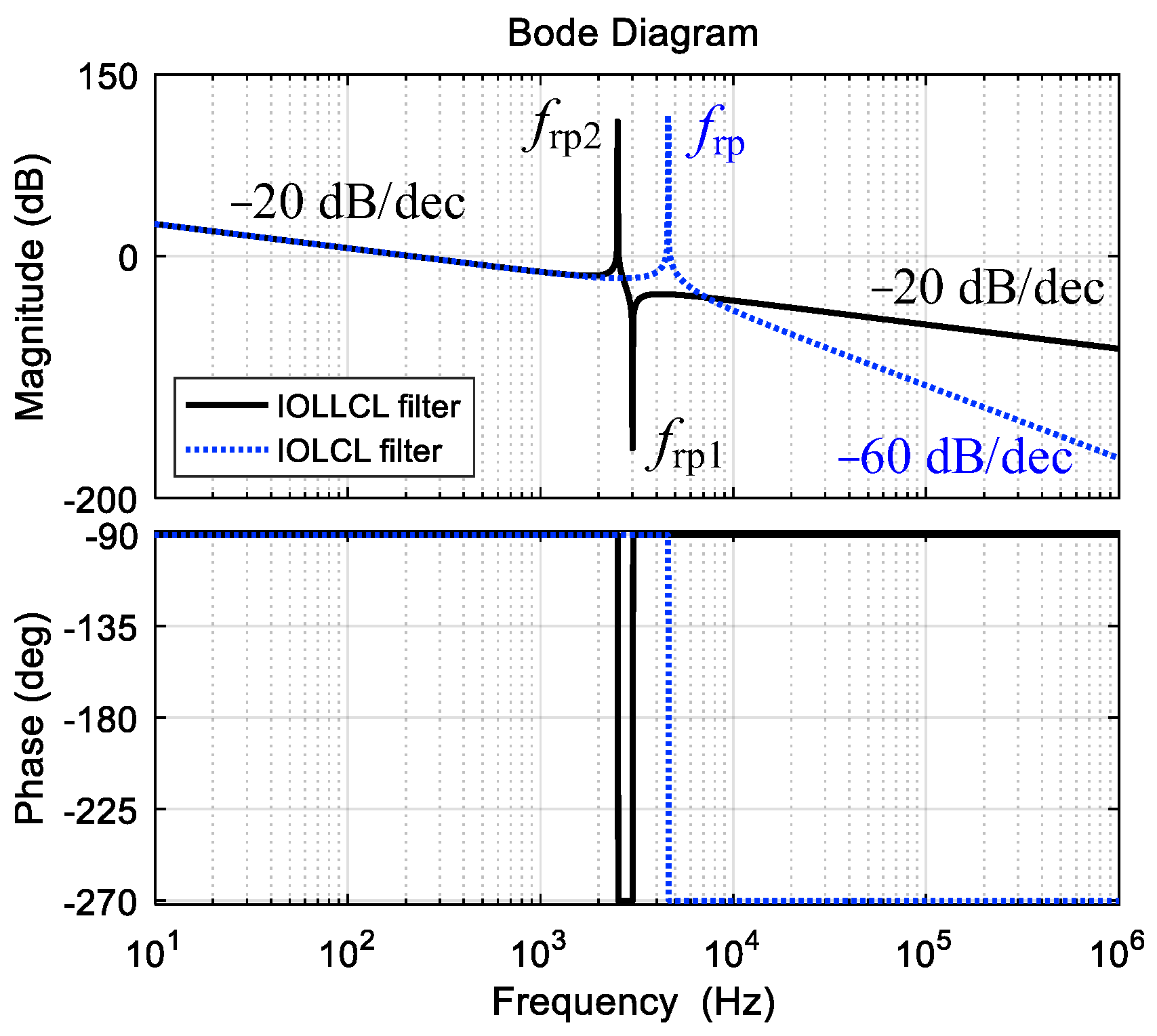
2. Integer-Order LLCL Filter

An VSI can connect the power grid through an LLCL filter to form a grid-tied inverter. The equivalent circuit of a single-phase integer-order LLCL-filter-based grid-tied inverter is shown in Figure 1, where L1 and L2 are the inverter-side and grid-side inductors, a small inductor Lf and a capacitor Cf composing a series resonant circuit, ui and i1 are the inverter output voltage and current, ug and ig are the grid voltage and current, and ic is the capacitor current.
The transfer function ig(s)/ui(s) of the IOLLCL filter can be derived as
G IO = i g ( s ) u i ( s ) | u g ( s ) = 0 = L f C f s 2 + 1 ( L 1 L 2 C f + ( L 1 + L 2 ) C f L f ) s 3 + ( L 1 + L 2 ) s
Figure 2 illustrates the bode diagrams of ig(s)/ui(s) for both the IOLLCL filter and IOLCL filter while all the other parameters are the same except for Lf. The specific parameters of the filters are given in Table 1. Unlike the IOLCL filter, the IOLLCL filter has two resonance peaks: a negative one and a positive one; the resonance frequencies are frp1 (ωrp1) and frp2 (ωrp2), respectively. When the VSI operates under the condition of the dual-carrier sine-wave PWM, the uppermost harmonics of ig are around the switching frequency 2fs. Therefore, frp1 is designed to be equal to 2fs to attenuate such harmonics. The positive resonance peak at frp2, as in the resonance peak at frp for the IOLCL filter, would lead to system instability in grid-tied inverter applications and should be damped by passive or active methods.
The negative resonant frequency of the IOLLCL filter is
ω rp 1 = 1 L f C f
The positive resonant frequency of the IOLLCL filter is
ω rp 2 = L 1 + L 2 L 1 L 2 C f + L f C f ( L 1 + L 2 )
It can also be seen from Figure 2 that the IOLLCL and IOLCL filters have similar low-frequency magnitude characteristics, while the IOLCL filter exhibits a better attenuation ability at a high-frequency band than the IOLLCL filter. However, overall, compared with the IOLCL filter, the grid current can obtain lower total harmonic distortion with the IOLLCL filter.

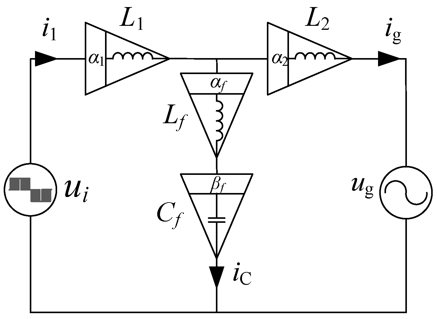
3. Fractional-Order LLCL Filter

The IOLLCL filter in the grid-tied inverter can be replaced by an FOLLCL filter to achieve better performance. The FOLLCL filter consists of four components: three inductors and a capacitor, as shown in Figure 3. In this paper, an LLCL filter can be called a fractional-order LLCL filter, with all or part of its components being fractional-order ones.
The transfer function from input (inverter output voltage ui) to output (grid current ig) is expressed as
G FO = i g ( s ) u i ( s ) = L f C f s α f + β f + 1 L 1 L 2 C f s α 1 + α 2 + β f + C f L f L 1 s α 1 + α f + β f + C f L f L 2 s α 2 + α f + β f + L 1 s α 1 + L 2 s α 2
where α1, α2, αf, and βf are the orders of L1, L2, Lf, and Cf, respectively. The magnitude–frequency and phase–frequency characteristic expressions obtained from (4) are quite complex. To simplify the analysis, set α1 = α2 = α; (4) is rewritten as
G FO = i g ( s ) u i ( s ) = L f C f s α f + β f + 1 L 1 L 2 C f s 2 α + β f + C f L f ( L 1 + L 2 ) s α + α f + β f + ( L 1 + L 2 ) s α = L f C f s α f + β f + 1 L 1 L 2 C f s α [ s α + β f + B s α f + β f + A ]
where A = (L1 + L2)/(L1L2Cf) and B = Lf (L1 + L2)/(L1L2). Substitute ()α = ωαcos(απ/2) + αsin(απ/2) into (5); the mathematical model in frequency domain can be obtained as
G FO ( j ω ) = L f C f ω α f + β f [ cos ( α f + β f ) π 2 + j sin ( α f + β f ) π 2 ] + 1 L 1 L 2 C f ω α ( cos α π 2 + j sin α π 2 ) [ ω α + β f cos ( α + β f ) π 2 + A + j ω α + β f sin ( α + β f ) π 2 + B ω α f + β f cos ( α f + β f ) π 2 + j B ω α f + β sin ( α f + β f ) π 2 ]
The magnitude–frequency characteristic of GFO is expressed as
| G FO ( j ω ) | = 1 L 1 L 2 C f ω α [ L f C f ω α f + β f cos ( α f + β f ) π 2 + 1 ] 2 + ( sin ( α f + β f ) π 2 ) 2 ( ω α + β f cos ( α + β f ) π 2 + A + B ω α f + β f cos ( α f + β f ) π 2 ) 2 + ( ω α + β f sin ( α + β f ) π 2 + B ω α f + β sin ( α f + β f ) π 2 ) 2

3.1. Resonant Frequencies

Define angular frequency ωr1 as follows:
ω r 1 = [ 1 L f C f cos [ ( α f + β f ) π / 2 ] ] 1 α f + β f
Then, the numerator of (7) can be expressed as
num ( | G FO | ) = [ ( ω ω r 1 ) α f + β f + 1 ] 2 + ( sin ( α f + β f ) π 2 ) 2
When ω = ωr1, (9) can be reduced to
num ( | G FO | ) = | sin ( α f + β f ) π 2 |
If αf + βf = 2n (n is an integer), sin[(αf + βf) nπ/2] = 0, and |GFO(r1)| as shown in (7) is zero. It means that the magnitude–frequency characteristic of the FOLLCL filter has a negative resonance (series resonance) peak at ω = ωr1. According to the present literature, the orders of the actually realizable fractional-order inductors and capacitors are greater than 0 and less than 2, so n is set to 1 in this research. Therefore, to attenuate the switching-frequency current ripple in grid-tied inverter applications, the sum of αf and βf must equal 2. Substitute αf + βf = 2 back into (8); the negative resonant frequency can be obtained as
ω rp 1 = 1 L f C f
It can be seen from (8) that the series resonance peak of the FOLLCL filter has the same form as the IOLLCL filter when αf + βf = 2. Series resonance is the most critical feature for the FOLLCL filter, so the following analysis is based on the relationship of αf + βf = 2.
Substitute αf + βf = 2 to (7); the denominator of (7) is expressed as
den ( | G FO | ) = L 1 L 2 C f ω α ( ω α + β f cos ( α + β f ) π 2 + A B ω 2 ) 2 + ( ω α + β f sin ( α + β f ) π 2 ) 2
Define angular frequency ωr2 as follows:
ω r 2 = [ A B ω 2 cos [ ( α + β f ) π / 2 ] ] 1 α + β f
Therefore, (12) can be expressed as
den ( | G FO | ) = L 1 L 2 C f ω α [ ( ω ω r 2 ) α + β f ( A B ω 2 ) + A B ω 2 ] 2 + ( ω α + β f sin ( α + β f ) π 2 ) 2
When ω = ωr2, (14) can be reduced to
den ( | G FO | ) = L 1 L 2 C f ω α ( ω r 2 α + β f sin ( α + β f ) π 2 ) 2
If α + βf = 2, sin[(α + βf)π/2] = 0, and |GFO(r2)| as shown in (7) is positive infinity. It means that the magnitude–frequency characteristic of the FOLLCL filter has a positive resonance peak at ω = ωr2. Substitute α + βf = 2 back into (13); the positive resonant frequency can be obtained as
ω rp 2 = L 1 + L 2 L 1 L 2 C f + L f C f ( L 1 + L 2 )
It can be seen from (16) that the FOLLCL filter has the same expression of positive resonance peak as the IOLLCL filter when αf + βf = 2 and α + βf = 2.
Theorem 1.
When α1 = α2 = α, the negative resonance (series resonance) peak of the FOLLCL filter exists only when αf + βf = 2; the resonant frequency is ω rp 1 = 1 / L f C f . The positive resonance peak of the FOLLCL filter exists only when αf + βf = 2 as well as α + βf = 2; the resonant frequency is ω rp 2 = ( L 1 + L 2 ) / [ L 1 L 2 C f + L f C f ( L 1 + L 2 ) ] . The positive resonant frequency ωrp2 is always less than the negative resonant frequency ωrp1.
Theorem 1 essentially reveals the resonant conditions for FOLLCL filters and provides a criterion to estimate whether an FOLLCL filter has resonance peaks. Orders α, αf, and βf of a conventional IOLLCL filter are all equal to 1. Both conditions αf + βf = 2 and α + βf = 2 are satisfied; therefore, the IOLLCL filter is just a special case of the FOLLCL filter. Moreover, the positive resonance peak can be avoided according to Theorem 1 by choosing reasonable orders for the inverter-side inductor L1, grid-side inductor L2, and capacitor Cf. Passive or active damping approaches used in an IOLLCL filter can be omitted for an FOLLCL filter.

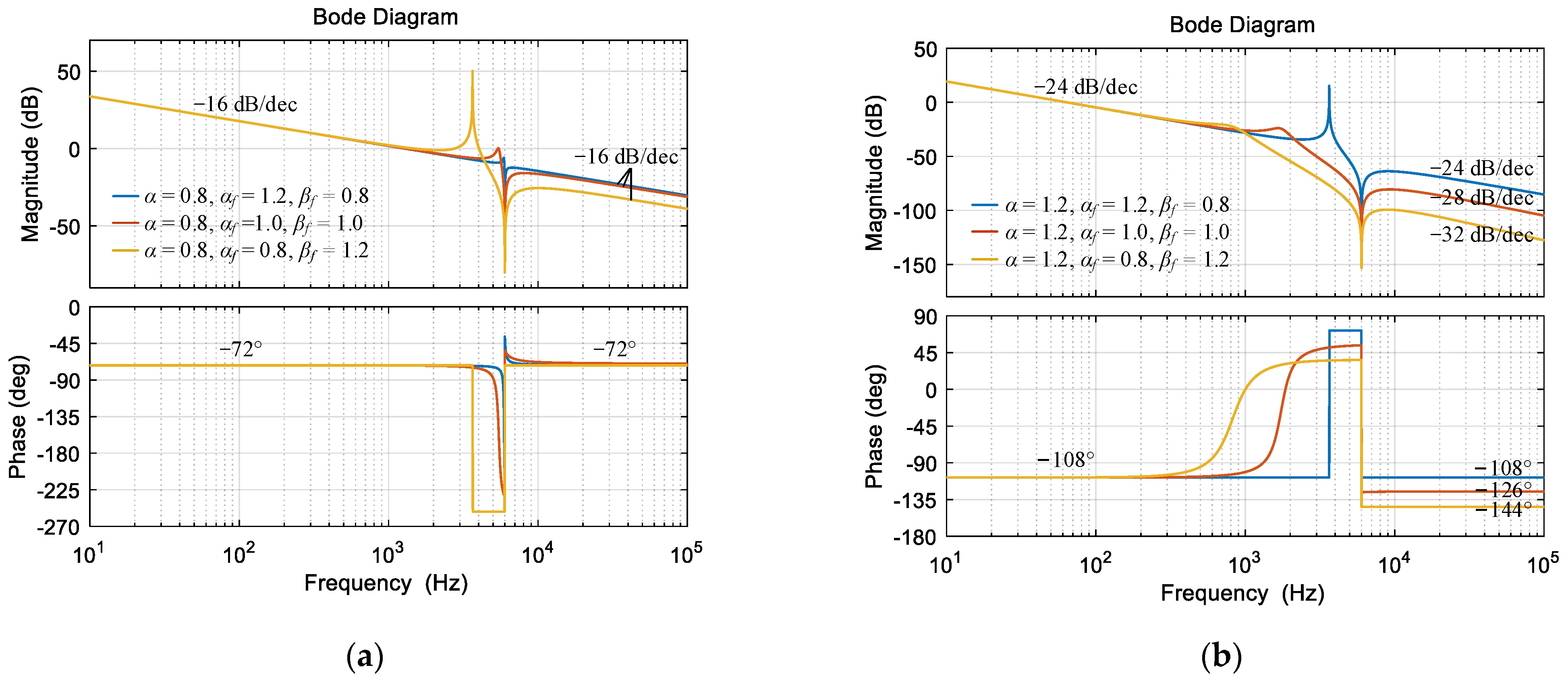
3.2. Magnitude–Frequency Characteristic

As previously mentioned, αf + βf = 2 must be satisfied for the FOLLCL filter, so (7) can be arranged as
| G FO ( j ω ) | = 1 L 1 L 2 C f ω α | L f C f ω 2 + 1 | ( ω α + β f + ( A B ω 2 ) cos ( α + β f ) π 2 ) 2 + ( A B ω 2 ) 2 sin 2 ( α + β f ) π 2  
(1) When ω << ωrp2, LfCfω2 << 1, and A2A, (17) can be further expressed as
| G FO ( j ω ) | = 1 L 1 L 2 C f ω α 1 ( ω α + β f + A cos ( α + β f ) π 2 ) 2 + A 2 sin 2 ( α + β f ) π 2
Define intermediate variables ωt1 and ωt2 as follows:
ω t 1 = | A cos ( α + β f ) π 2 | 1 α + β f
ω t 2 = | A sin ( α + β f ) π 2 | 1 α + β f
Substitute (19) and (20) into (18); the magnitude–frequency characteristic can be derived as
| G FO ( j ω ) | = 1 L 1 L 2 C f ω α 1 ( ω α + β f + τ ω t 1 α + β f ) 2 + ω t 2 2 ( α + β f )
where τ = 1 (α + βf ∈ (0, 1] ∪ [3, 4)) or τ = −1 (α + βf ∈ (1, 3)).
When ω << ωt1, ( ω / ω t 1 ) α + β f 0 and τ2 = 1, (21) can be simplified as
| G FO ( j ω ) | = 1 L 1 L 2 C f ω α ω t 1 α + β f 1 ( ( ω / ω t 1 ) α + β f + τ ) 2 + ( ω t 2 / ω t 1 ) 2 ( α + β f ) 1 L 1 L 2 C f ω α 1 ω t 1 2 ( α + β f ) + ω t 2 2 ( α + β f ) = 1 L 1 L 2 C f A ω α
The log magnitude–frequency characteristic and the slope of its asymptote are expressed as (23) and (24).
L ( ω ) 20 lg ( L 1 L 2 C f A ) 20 α lg ω
d L ( ω ) d lg ω 20 α   dB / dec , ω < < ω t 1
(2) When ω >> ωrp1, LfCfω2 >> 1, and A22, (17) can be expressed as
| G FO ( j ω ) | = 1 L 1 L 2 C f ω α L f C f ω 2 ( ω α + β f + B ω 2 cos ( α + β f ) π 2 ) 2 + B 2 ω 4 sin 2 ( α + β f ) π 2
ω t 3 = | B cos ( α + β f ) π 2 | 1 α + β f
Define intermediate variables ωt3 and ωt4 as follows:
ω t 4 = | B sin ( α + β f ) π 2 | 1 α + β f
Substitute (26) and (27) into (25); the magnitude–frequency characteristic can be derived as
| G FO ( j ω ) | = 1 L 1 L 2 C f ω α L f C f ω 2 ( ω α + β f + τ ω 2 ω t 3 α + β f ) 2 + ω 4 ω t 4 2 ( α + β f )
When ω >> ωrp1 and α + βf ∈ [2, 4), ω 2 ( ω t 3 / ω ) α + β f 0 , and ω 2 ( ω t 4 / ω ) α + β f 0 , (17) can be expressed as
| G FO ( j ω ) | = 1 L 1 L 2 C f ω 2 α + β f L f C f ω 2 ( 1 + τ ω 2 ( ω t 3 / ω ) α + β f ) 2 + ω 4 ( ω t 4 / ω ) 2 ( α + β f ) L f L 1 L 2 ω 2 α + β f 2
The log magnitude–frequency characteristics and the slope of its asymptote are expressed as (30) and (31).
L ( ω ) 20 lg L f 20 lg ( L 1 L 2 ) 20 ( 2 α + β f 2 ) lg ω
d L ( ω ) d lg ω 20 ( 2 α + β f 2 )   dB / dec ,   ω > > ω rp 1
Similarly, when ω >> ωrp1 and α + βf ∈ (0,2), the slope of the asymptote is −20α dB/dec.
Theorem 2.
For FOLLCL, when ω << ωrp2, the asymptote slope of the low-frequency log magnitude–frequency characteristic is −20α dB/dec. When ω >> ωrp1, α + βf∈ [2, 4), the asymptote slope of the high-frequency log magnitude–frequency characteristics is −20 (2α + βf − 2) dB/dec; if α + βf∈ (0, 2), the asymptote slope is −20α dB/dec.

3.3. Phase–Frequency Characteristic

According to (6), when αf + βf = 2, the phase model can be expressed as
G FO ( j ω ) = arctan ( tan π α 2 ) arctan ω α + β f sin ( α + β f ) π 2 ω α + β f cos ( α + β f ) π 2 + A B ω 2
(1) When ω << ωt1, A − Bω2 ≈ A and ω α + β f sin [ ( α + β f ) π / 2 ] << ω α + β f cos [ ( α + β f ) π / 2 ] + A , so the low-frequency phase is expressed as
G FO ( j ω ) arctan ( tan π α 2 ) arctan ω α + β f sin ( α + β f ) π 2 ω α + β f cos ( α + β f ) π 2 + A π α 2
(2) When ω >> ωrp1, A − Bω2 ≈ −Bω2 and Bω2 << | ω α + β f cos [ ( α + β f ) π / 2 ] |. Moreover, when α + βf ∈ [2, 4), arctan { tan [ ( α + β f ) π / 2 ] } = ( α + β f ) π / 2 2 π , so the high-frequency phase is expressed as
G FO ( j ω ) π arctan ( tan π α 2 ) arctan ω α + β f sin ( α + β f ) π 2 ω α + β f cos ( α + β f ) π 2 B ω 2 π arctan ( tan π α 2 ) arctan ω α + β f sin ( α + β f ) π 2 ω α + β f cos ( α + β f ) π 2 = π ( α + β f / 2 ) + π
When α + βf ∈ (0,2), ω α + β f sin [ ( α + β f ) π / 2 ] << | ω α + β f cos [ ( α + β f ) π / 2 ] B ω 2 | , so the high-frequency phase can be expressed as
G FO ( j ω ) arctan ( tan π α 2 ) arctan ω α + β f sin ( α + β f ) π 2 ω α + β f cos ( α + β f ) π 2 B ω 2 π α 2
Theorem 3.
For FOLLCL, when ω << ωrp2, the low-frequency phase is −πα/2. When ω >> ωrp1, if α + βf∈ [2, 4),the high-frequency phase is −π (α + βf/2) + π; if α + βf∈ (0, 2), the high-frequency phase is −πα/2.
It can be seen from Theorem 2 and Theorem 3 that the low-frequency characteristics only depend on the orders of L1 and L2, and are independent of the orders of Lf and Cf. The high-frequency characteristics are determined by the orders of L1, L2, and Cf when α + βf ∈ [2, 4), and only depend on the orders of L1 and L2 when α + βf ∈ (0, 2).

3.4. Simulation Analyses

The bode plots of the FOLLCL filter are shown in Figure 4. The specific parameters of the FOLLCL filter are given in Table 1. Two cases are considered, namely, α + βf ≤ 2 and α+βf ≥ 2. The values of the asymptote slopes and phases are marked in the plots; it can be seen that the results are consistent with the theoretical analyses. In particular, the positive resonance peak is suppressed when α + βf ≠ 2. Furthermore, it is shown in Figure 4b that when α + βf > 2, the phase–frequency characteristic curves do not pass through −180°, which means that the phase crossover frequency does not exist. Therefore, α + βf must be less than or equal to 2 to guarantee the stability.

4. Grid-Tied Inverter Based on Fractional-Order LLCL Filter

An FOLLCL filter and a VSI can be combined to form a grid-tied inverter. Figure 5 shows the single-phase FOLLCL-type grid-tied inverter and its control system. The primary objective of the grid-tied inverter is to control the grid-side current ig to be synchronized with the grid voltage, which is denoted by ug. I* is the reference amplitude of the grid-side current, θ is the phase of grid voltage obtained by the phase-locked loop (PLL), and i g * is the reference of the grid-side current. ig is sensed with the sensor gain of Hig and compared with i g * . The current error is sent to the current regulator Gi; Gi = Kp + Ki/sλ, and Kp, Ki, and λ are the proportional coefficient, integral coefficient, and order of the integrator, respectively. For the FOLLCL filter with α + βf equaling or very close to 2, an active damping method is used to attenuate the positive resonance. The output of Gi is sent to the PWM generator after subtracting the capacitor current iC, which is sensed with the sensor gain of HiC. For the FOLLCL filter with α + βf deviating from 2, the output of Gi is sent to the PWM generator directly; the active damping can be avoided.

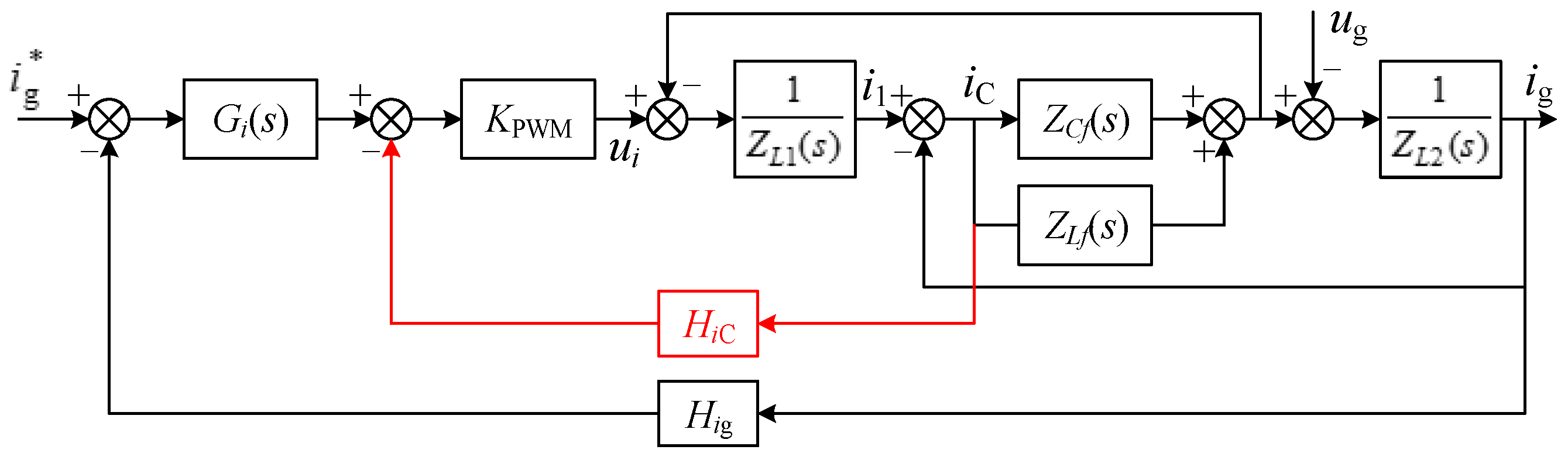
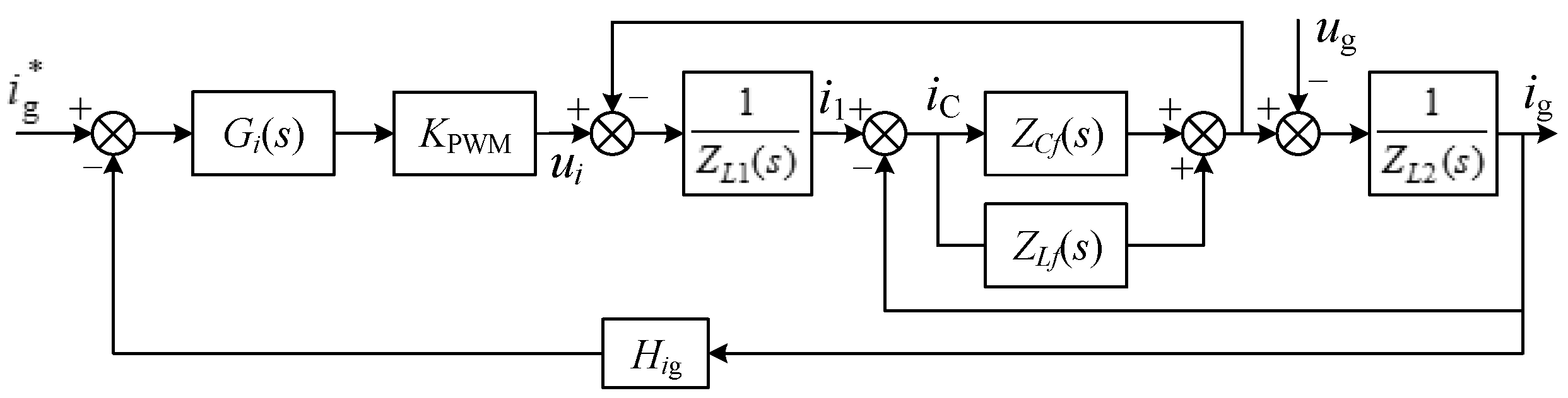
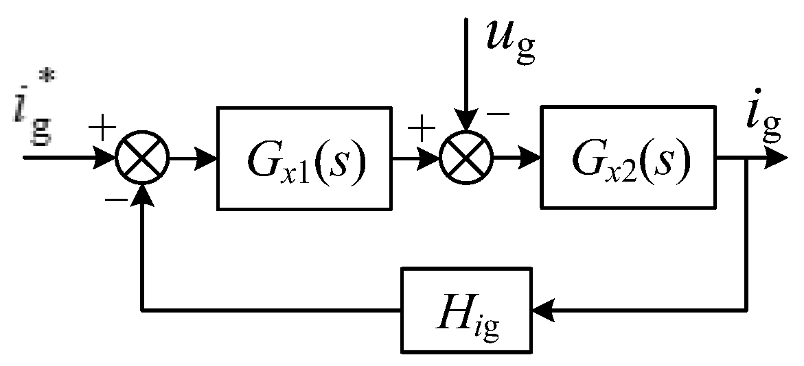
4.1. Structure of the Control System

According to Figure 5, the control block diagram of the single-phase FOLLCL-type grid-tied inverter when α + βf equals to or is very close to 2 is shown in Figure 6, where KPWM is the transfer function from the modulation signal to the inverter output voltage, expressed as KPWM = udc/Vtri, and Vtri is the amplitude of triangular carrier. ZL1(s), ZL2(s), ZLf(s), and ZCf(s) are the impedance of L1, L2, Lf, and Cf, respectively, which are expressed as
Z L 1 ( s ) = s α L 1 , Z L 2 ( s ) = s α L 2 , Z L f ( s ) = s α f L 1 , Z C f ( s ) = 1 / s β f C f
The control block diagram of the single-phase FOLLCL-type grid-tied inverter when α+βf deviates from 2 is shown in Figure 7. Compared with Figure 6, the capacitor current feedback loop is removed.
The control block diagrams in Figure 6 and Figure 7 can be equivalently transformed into the block diagram in Figure 8. The transfer functions Gx1 and Gx2 are expressed as (37) and (38), respectively:
G x 1 ( s ) = K PWM G i ( s ) [ Z L f ( s ) + Z C f ( s ) ] Z L 1 ( s ) + Z L f ( s ) + Z C f ( s ) + H i C K PWM
G x 2 ( s ) = Z L 1 ( s ) + Z L f ( s ) + Z C f ( s ) + H i C K PWM Z L 1 ( s ) Z L 2 ( s ) + [ Z L 1 ( s ) + Z L 2 ( s ) ] [ Z L f ( s ) + Z C f ( s ) ] + H i C K PWM Z L 2 ( s )
where HiC = 0 when α + βf ≠ 2.
According to the equivalent block diagram in Figure 8 and (36)~(38), the expression of the loop gain can be derived as
T A ( s ) = G x 1 ( s ) G x 2 ( s ) H i g ( s ) = H i g K PWM G i ( s ) ( L f C f s α f + β f + 1 ) L 1 L 2 C f s 2 α + β f + ( L 1 + L 2 ) L f C f s α + α f + β f + L 2 C f H i C K PWM s α + β f + ( L 1 + L 2 ) s α
As discussed in Part 3, αf + βf = 2 must be satisfied in grid-tied inverter applications, so (39) is rewritten as
T A ( s ) = H i g K PWM G i ( s ) ( L f C f s 2 + 1 ) L 1 L 2 C f s 2 α + β f + ( L 1 + L 2 ) L f C f s α + 2 + L 2 C f H i C K PWM s α + β f + ( L 1 + L 2 ) s α
The grid current ig can be expressed as
i g ( s ) = 1 H i g T A ( s ) 1 + T A ( s ) i g * ( s ) G x 2 ( s ) 1 + T A ( s ) u g ( s ) = i g 1 ( s ) + i g 2 ( s )
It can be seen from (41) that ig(s) consists of two parts: the reference tracking component ig1(s) and the disturbance component ig2(s) caused by the grid voltage, which can be expressed as (42) and (43), respectively.
i g 1 ( s ) = 1 H i g T A ( s ) 1 + T A ( s ) i g * ( s )
i g 2 ( s ) = G x 2 ( s ) 1 + T A ( s ) u g ( s )

4.2. System Performance Analysis

The loop gain at the fundamental frequency is often much greater than one, so 1 + TA(s) ≈ TA(s), and (42) can be rewritten as i g 1 ( s ) i g * ( s ) / H i g . Therefore, ig1(s) and i g * ( s ) are almost in phase. For ffc, the LfCf branch can be considered open. According to (38) and (40), the expression of Gx2(s) and TA(s) at the fundamental frequency can be obtained as follows:
G x 2 ( j 2 π f o ) 1 ( j 2 π f o ) α ( L 1 + L 2 )
T A ( j 2 π f o ) H i g K PWM G i ( j 2 π f o ) ( j 2 π f o ) α ( L 1 + L 2 )
where fo is the fundamental frequency. Substitute (44) and (45) into (43), and for PI regulator, Gi(jfo) ≈ Ki/(jfo), so we have
i g 2 u g H i g K PWM G i ( j 2 π f o ) j 2 π f o u g H i g K PWM K i
From (46), it can be seen that ig2 lags behind ug by 90°; a small ig2 is expected to reduce the amplitude and phase tracking errors for ig. From (45) and (46), the RMS value of ig2 can be expressed as
I g 2 U g H i g K PWM | G i ( j 2 π f o ) | U g ( 2 π f o ) α ( L 1 + L 2 ) | T A ( j 2 π f o ) |
The magnitude of the loop gain at fo is expressed as
T fo = 20 l g | T A ( j 2 π f o ) | 20 l g U g ( 2 π f o ) α ( L 1 + L 2 ) I g 2  
where the unit of Tfo is dB. Thus, the steady-state error requirement for Ig2 is converted to the requirement for Tfo. Obviously, for a given value of Ig2, a smaller-order α means bigger Tfo.
Compared to the PI regulator, the PR regulator can significantly increase Tfo, and thus decrease the steady-state error of the grid current. The expression of the PR regulator is
G i ( s ) = K p + 2 K r ω i s s 2 + 2 ω i s + ω o 2
where Kp is the proportional coefficient, Kr is the resonant coefficient, ωi is the bandwidth concerning the –3 dB cutoff frequency of the resonant compensator, and ωo = 2πfo is the fundamental angular frequency. The design criteria of the PR regulator have been reported in many works in the literature and will not be repeated here.
In order to demonstrate the control system design criteria of the FOLLCL-type grid-tied inverter, four cases are presented based on the system parameters listed in Table 1 and Table 2.
Case I (α + βf = 2, PI control): For α + βf = 2 (taking (α, αf, βf) = (1.2, 1.2, 0.8) and (α, αf, βf) = (1.1, 1.1, 0.9) as examples), the bode diagrams of the loop gain before compensation (Gi(s) = 1) are drawn in Figure 9 according to (40), where fc is the cut-off frequency of the loop gain. As shown in Figure 9, the capacitor current feedback can effectively suppress the positive resonance peak of the FOLLCL filter, and the resonance damping capability becomes stronger with the increase of HiC. As with the application in conventional IOLCL-type grid-tied inverters, this well-known active damping method only changes the magnitude–frequency characteristics around the resonant frequency frp2. However, the phase–frequency characteristics vary observably; they decrease from –(90α)° when f < frp2.
The control system parameter design principles for IOLCL-type grid-tied inverters are adopted here to control the FOLLCL-type grid-tied inverter with α + βf = 2. The bode diagrams of the loop gain after compensation (Gi(s) = Kp + Ki/s) are shown in Figure 10. The frequency characteristics without active damping and compensation (green dotted lines) when (α, αf, βf) = (1.2, 1.2, 0.8) are also plotted in the same figure for comparison purpose. HiC = 0.1, Hig = 0.15, Kp = 0.45, and Ki = 2200 are designed in this case to yield a satisfactory overall system performance. Compared with the original system (green dotted lines), the loop gain at the fundamental frequency (Tfo) after compensation (blue solid lines) increases and the high-frequency (f > frp1) magnitude characteristics move down, which can guarantee the fundamental current tracking and high-frequency harmonic attenuation capabilities. It can also be seen from Figure 10 that a lower α can guarantee better performance under the condition of α + βf = 2. When α = 1.1, the system has a sufficient gain margin (GM = 5.04 dB) and an acceptable phase margin (PM = 38.1°, while PM > 45° is required for a well-designed system), as well as a reasonable cut-off frequency (fc = 948 Hz) and a sufficient fundamental loop gain (Tfo = 49.5 dB), while when α = 1.2, although there is a slightly higher gain margin (GM = 5.74 dB), the PM, fc, and Tfo all decrease. The low phase margin (PM = 17.1°) especially threatens the system stability.
Case II (α + βf ≠ 2, PI control): For α + βf ≠ 2 (taking α = 1.1, αf = 1.2, βf = 0.8 as an example), the bode diagrams of the loop gain before compensation (Gi(s) = 1) are drawn in Figure 11. HiC = 0 is set in this case to avoid active damping. The positive resonance peak is damped effectively by selecting appropriate values for orders α and βf to make their sum unequal to 2. When Hig = 0.15, the same value as in case I, the cut-off frequency is very close to the equivalent switching frequency 2fs (6 kHz), which is not acceptable for a grid-tied inverter. Moreover, when Hig = 0.1 or 0.15, the magnitude plot has three cut-off frequencies and the system behaves as a conditionally stable system. For a large Hig, even if the system can be stable after compensation, it is not easy to obtain a sufficient gain margin. If we keep decreasing Hig to 0.05, the magnitude plot has only one cut-off frequency. Therefore, Hig = 0.05 is chosen for the compensated system in the next step.
The bode diagrams of the loop gain after compensation (Gi(s) = Kp + Ki/sλ, λ = 1) are shown in Figure 12. As seen from (46), the decrease of Hig will increase ig2, so Ki should be increased to meet the steady-state error requirement. However, the phase margin when Ki = 2200 is only 22.7°, and after increasing Ki from 2200 to 4000, the phase margin decreases to 14.6°, and a sufficient phase margin cannot be guaranteed.
Case III (α + βf ≠ 2, PIλ control): In this case, (α, αf, βf) = (1.1, 1.2, 0.8), HiC = 0, Hig = 0.05, and a fractional-order PIλ regulator is used to try to improve the phase margin. When Kp = 0.45, Ki = 2200, and λ increases from 0.8 to 1.4, the bode diagrams of the loop gain are shown in Figure 13. The phase margin increases with λ, so λ = 1.4 is selected to leave enough room for Ki adjustment.
The bode diagrams of the loop gain with varying Ki when λ = 1.4 are shown in Figure 14. With the increase of Ki, the phase margin decreases, but it is still sufficient even Ki = 6000 (PM = 49.2°). However, each curve in Figure 13 and Figure 14 has a small Tfo, so the steady-state error requirement is still not guaranteed according to (47) and (48). The contradiction between Tfo and PM cannot be balanced by a PIλ regulator.
Case IV (α + βf≠2, PR control): In this case, (α, αf, βf) = (1.1, 1.2, 0.8), HiC = 0, Hig = 0.05, and a PR regulator is used to control the grid current. The values of the parameters are Kp = 0.45, ωo = 2π × 50 rad/s, and ωi = π rad/s, and Kr increases from 100 to 300; the bode diagrams of the compensated system are shown in Figure 15. It can be seen that each curve has a large enough Tfo to eliminate the steady-state error of ig. However, PM decreases with the increase of Kr, when Kr = 100, GM = 11.3 dB, PM is 59.3°, and the fc also has a good value, so Kr = 100 will be selected in the simulation section.
Based on the four cases discussed previously, it can be concluded that:
(1)
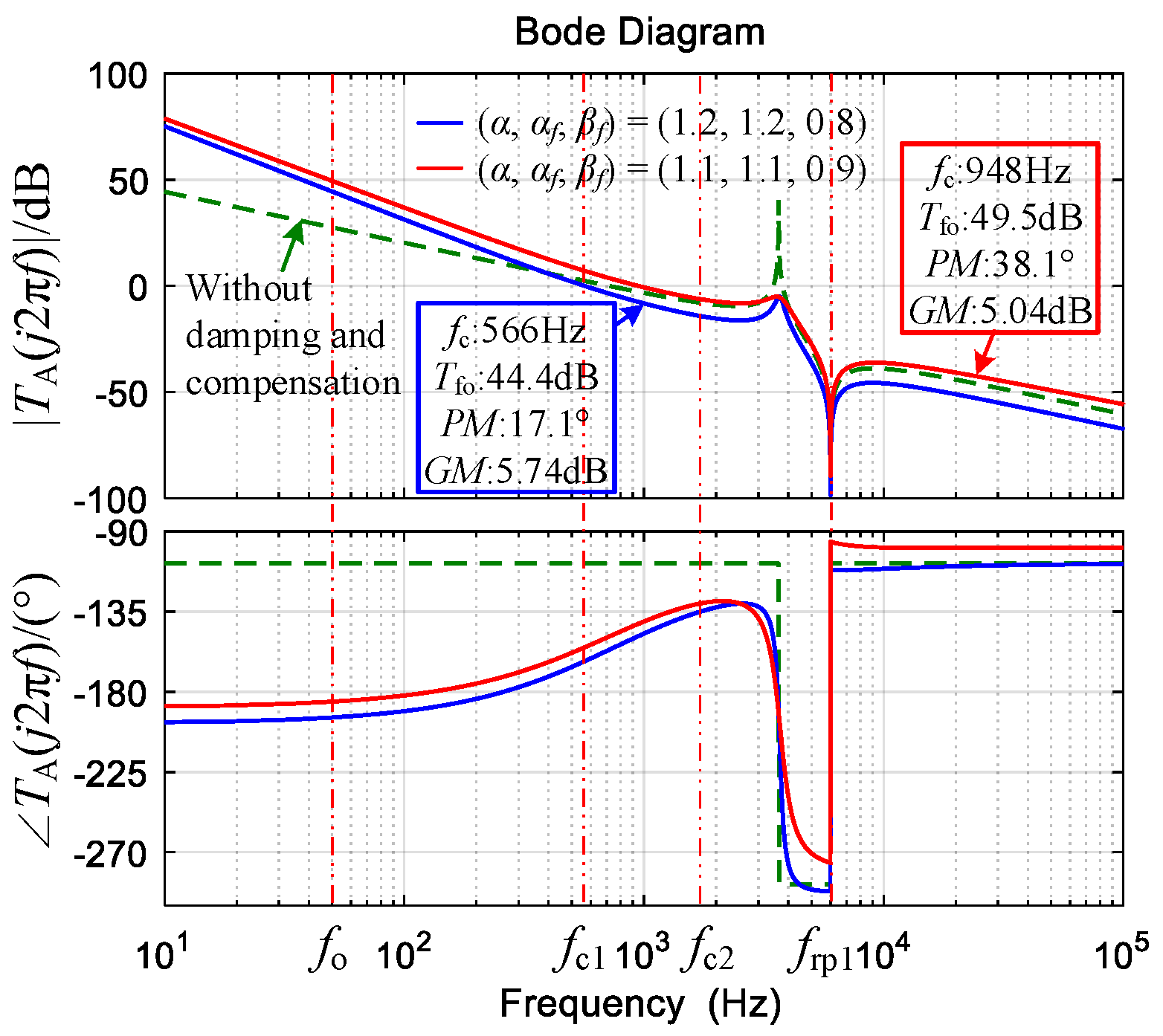
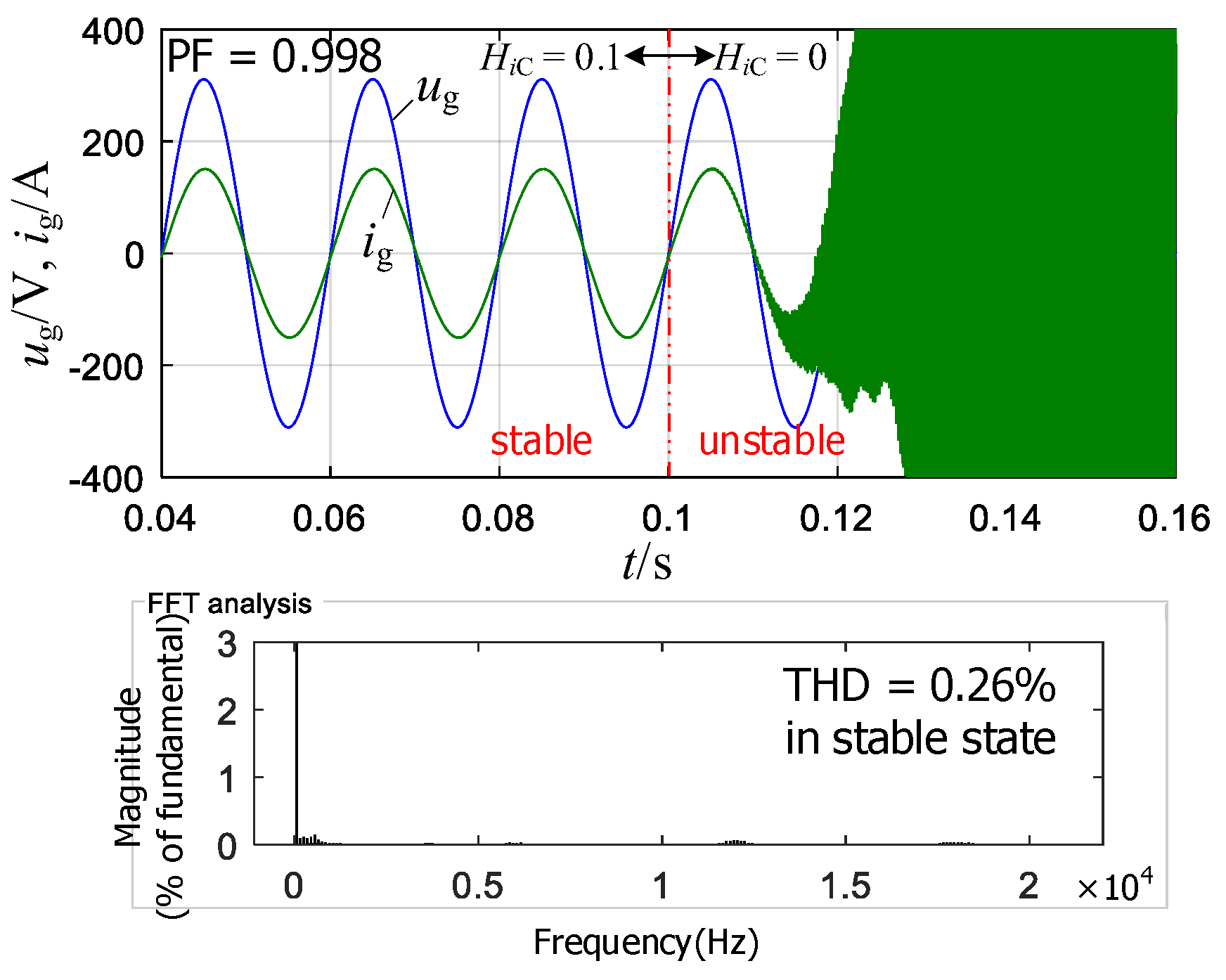
If α + βf = 2, the FOLLCL-type grid-tied inverter can be damped by a capacitor current feedback loop. Under PI control, a lower α can achieve a larger PM but a higher fc.
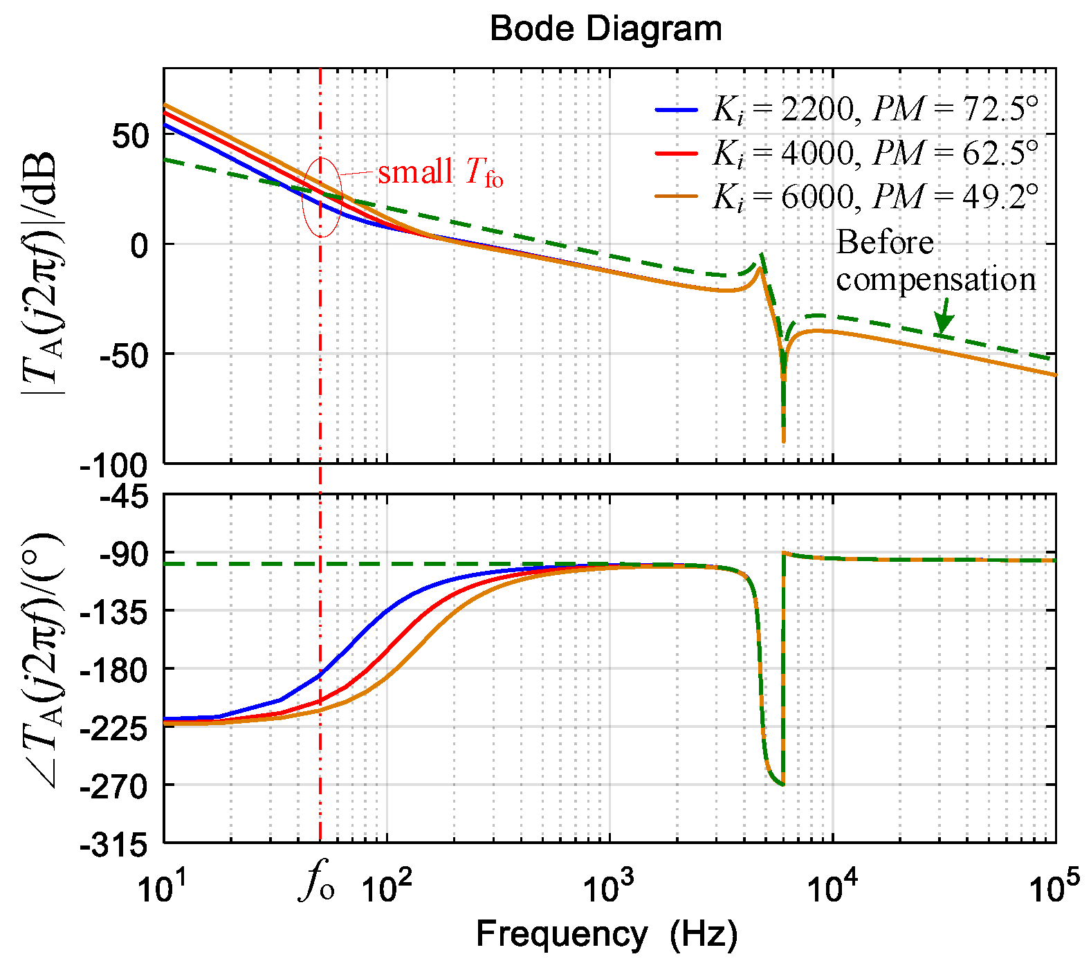
(2)
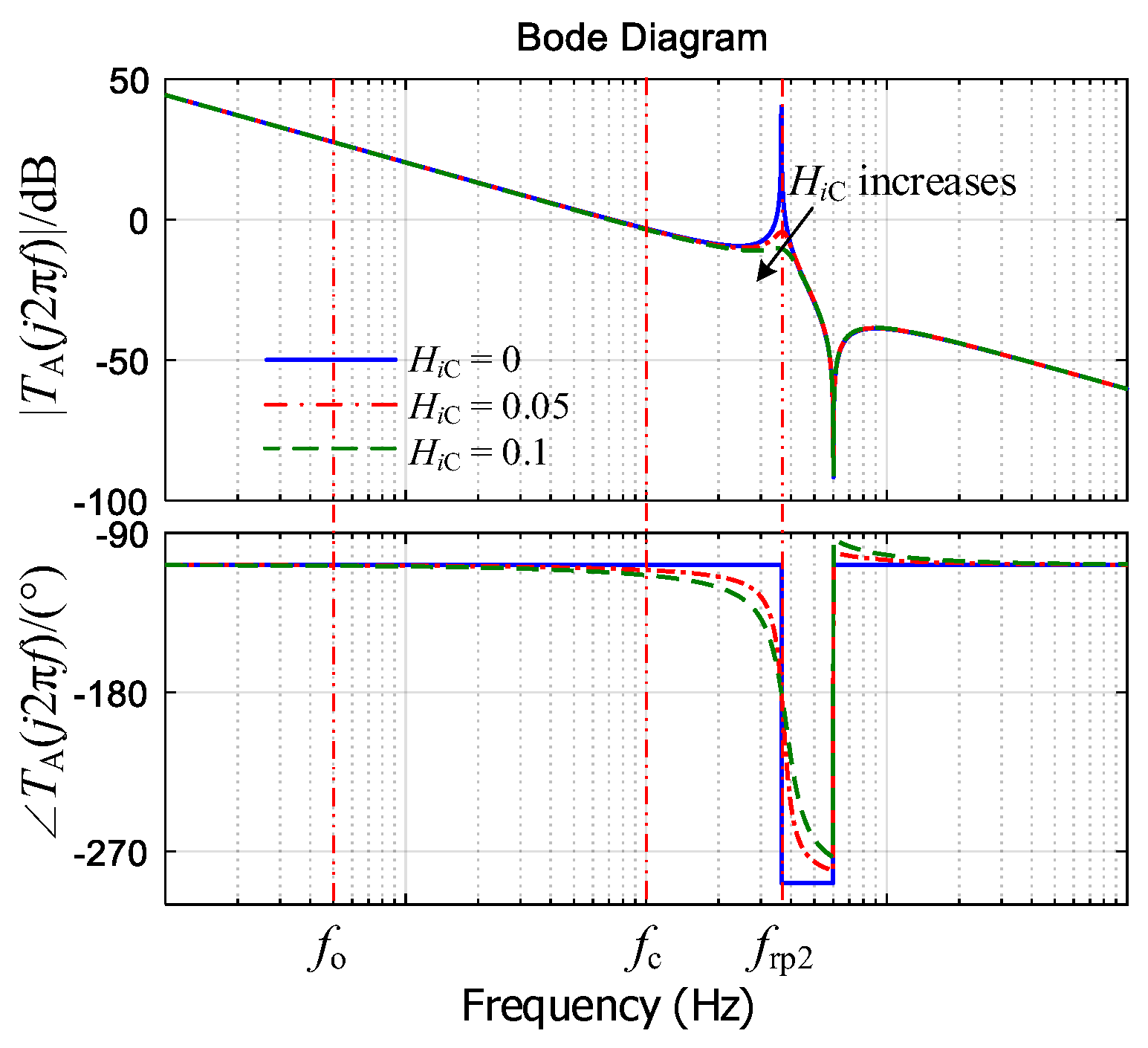
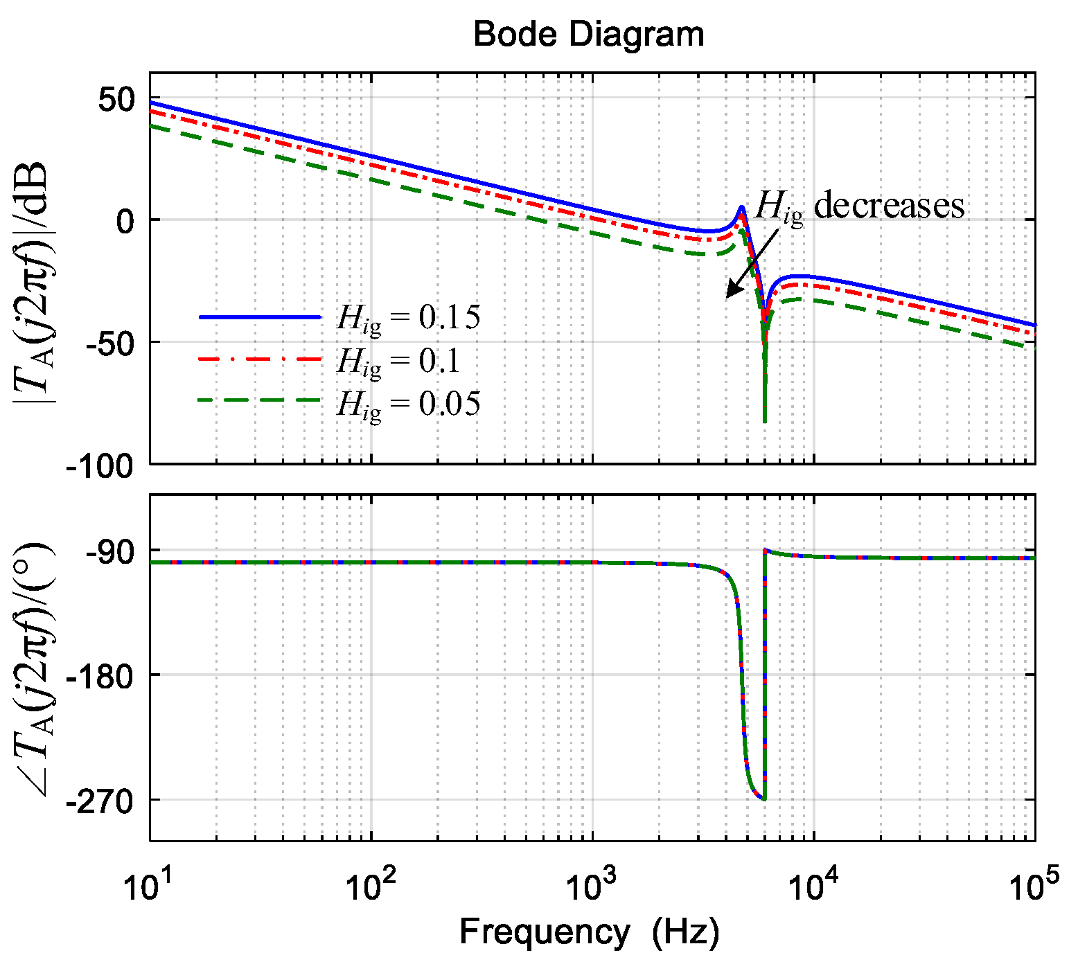
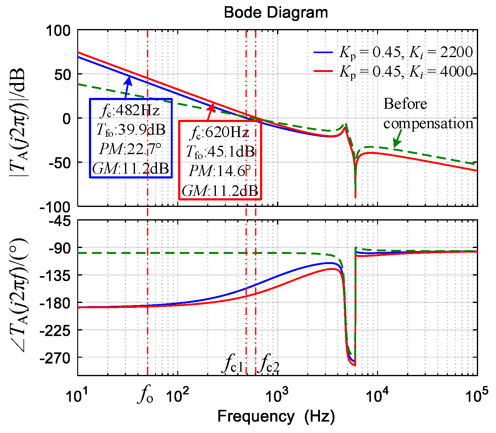
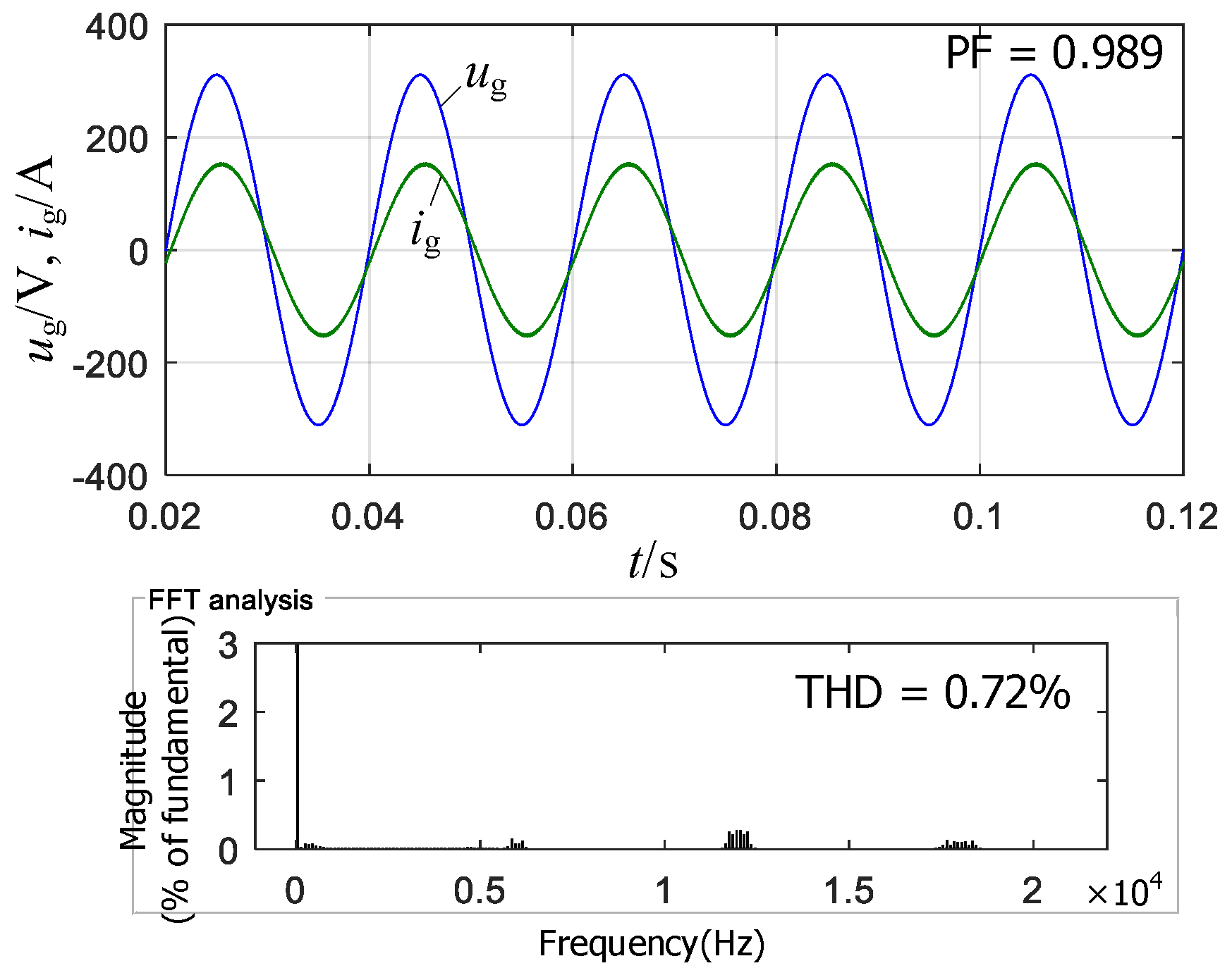
If α + βf ≠ 2, the system is stable under the grid current feedback; the capacitor current feedback is avoided. Under PI control, a large Ki should be chosen to reduce the steady-state error of ig, but the PM decreases significantly.
(3)
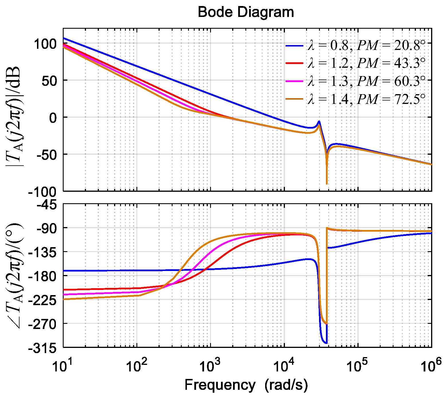
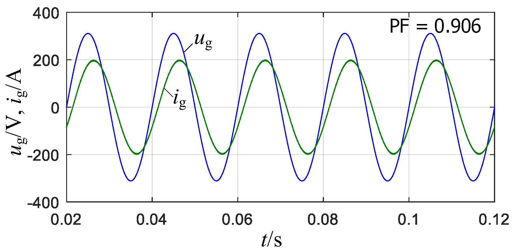
A PIλ regulator can also make the system stable, but there is a contradiction between Tfo and PM.
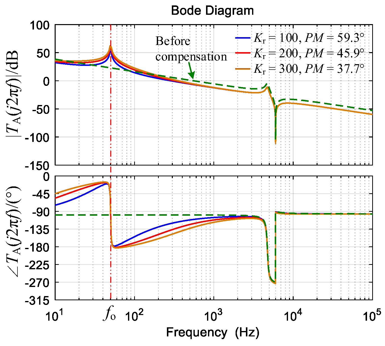
(4)
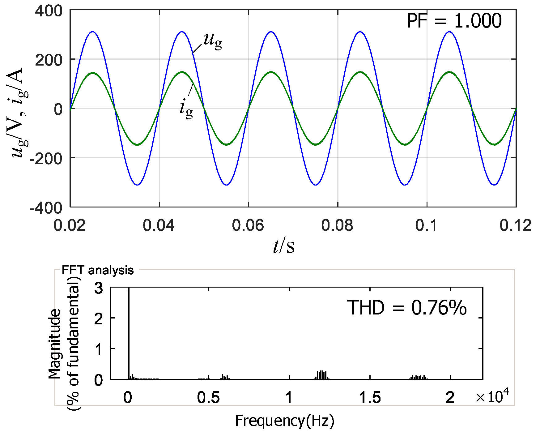
A PR regulator can simultaneously obtain good Tfo, GM, PM, and fc, which is suitable for controlling the FOLLCL-type grid-tied inverter if α + βf ≠ 2.
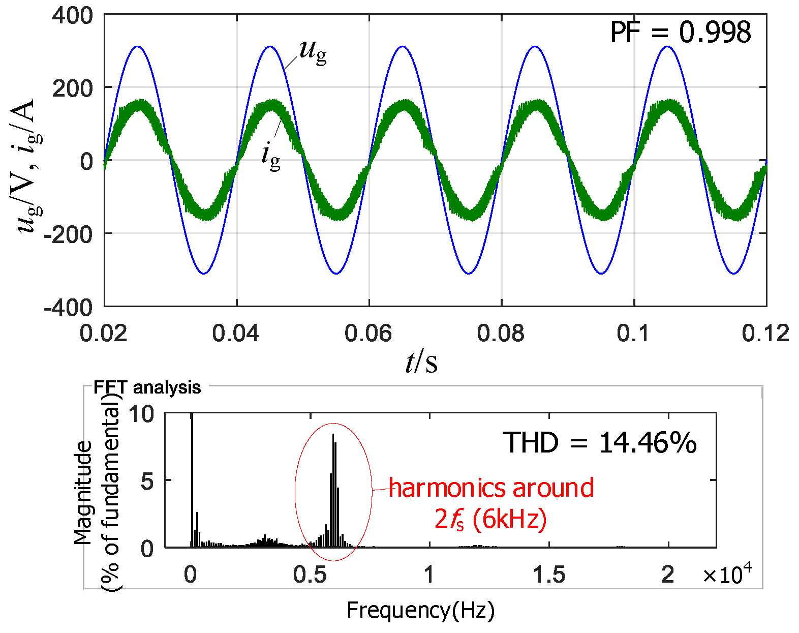
5. Simulations

To verify the characteristics of the FOLLCL-type grid-tied inverter and the effectiveness of the control methods, simulations are conducted with the parameters presented in Table 1 and Table 2. In each simulation, the reference grid current i g * is set to 50sin(ωt) A; ig is magnified three times for observation in the waveform diagram. The fractional-order inductors and capacitor are equivalent to the fractance circuit using the Oustaloup approximation method.In the first simulation, an IOLCL-type grid-tied inverter is studied. As shown in Figure 16, a large amount of harmonics, which is mainly around 2fs (6 kHz), exists in the grid current. The THD of ig is 14.46%, which is not acceptable in the application. The result indicates that the LCL-type grid-tied inverter has little advantage in low-frequency applications.
In the second simulation, an FOLLCL-type grid-tied inverter with α + βf = 2 and αf + βf = 2 (α = 1.1, αf = 1.1, βf = 0.9) under PI control is investigated. As shown in Figure 17, when the capacitor current feedback loop is effective before 0.1 s, the system is stable, the grid current has a very low THD (only 0.26%), and the power factor is high (0.998). The FOLLCL-type grid-tied inverter exhibits excellent harmonic suppression ability. However, instability arises after 0.1 s due to the removal of the capacitor current feedback loop, which causes positive resonance.
Moreover, an FOLLCL-type grid-tied inverter with α + βf ≠ 2 and αf + βf = 2 (α = 1.1, α = 0.2, βf = 0.8) is studied. The inverter is regulated by a PI controller; the control parameters are Kp = 0.45 and Ki = 2200, respectively. As with the analysis in Section 4 (case II), the capacitor current feedback is eliminated and Hig = 0.05. As shown in Figure 18, the system is stable without active damping and the grid current is close to the ideal sine, which has a THD of 0.72%. However, to obtain a sufficient phase margin, Ki cannot be too large, resulting in a certain phase error between ug and ig; the power factor is only 0.989.
Furthermore, in Figure 19, the simulation results of the FOLLCL-type grid-tied inverter with α + βf ≠ 2 and αf + βf = 2 (α = 1.1, αf = 1.2, βf = 0.8) controlled by a PIλ regulator are shown. According to the analysis in Section 4 and case III, when λ = 1.4 and Ki = 6000, although PM > 45°, the Tfo is very small, as can be seen in Figure 14. Therefore, as shown in Figure 19, both the amplitude error and phase error between i g * and ig are very large, and the power factor is only 0.906.
Finally, a PR regulator is used to control the FOLLCL-type grid-tied inverter with α + βf ≠ 2 and αf + βf = 2 (α = 1.1, αf = 1.2, βf = 0.8). Kp = 0.45, ωi = π, and Kr = 100 are the parameters of the regulator, and Hig = 0.05. The results are shown in Figure 20. The grid current is in strict in-phase with the grid voltage; the power factor is 1. In addition, the amplitude error is close to 0. The results are consistent with the previous analysis in Section 4.
The above simulation results prove that the analyses in previous sections are correct and PR regulator is superior to PI and PIλ regulators to control an FOLLCL-type grid-tied inverter with α + βf ≠ 2.

6. Conclusions

In this paper, the fractional-order LLCL filter and the grid-tied inverter based on it are studied. By correctly selecting the orders of the components, the positive resonance can be suppressed and the negative resonance is reserved. Therefore, the passive or active damping can be avoided for the FOLLCL-type grid-tied inverter. Meanwhile, the switching-frequency harmonics in the grid current can be attenuated. For low-frequency applications, it is difficult for the PI controller and fractional-order PI controller to balance all performances simultaneously. PR controllers can guarantee good fundamental frequency loop gain, cut-off frequency, gain margin, and phase margin at the same time. The FOLLCL-type grid-tied inverter without active damping under PR control achieves excellent tracking accuracy and low grid current THD. Simulations are conducted to verify the correctness of the theoretical analyses.

Author Contributions

Methodology, X.W.; Software, R.Z. and J.C.; Validation, R.Z. and J.C.; Investigation, X.W.; Writing—original draft, X.W.; Writing—review & editing, X.W. All authors have read and agreed to the published version of the manuscript.

Funding

This work was supported by the “Guangzhou Science and Technology Plan Project, no. 202102010404”.

Institutional Review Board Statement

Not applicable.

Informed Consent Statement

Not applicable.

Data Availability Statement

Not applicable.

Conflicts of Interest

The authors declare no conflict of interest.

References

  1. Twining, E.; Holmes, D.G. Grid current regulation of a three-phase voltage source inverter with an LCL input filter. IEEE Trans. Power Electron. 2003, 18, 888–895. [Google Scholar] [CrossRef] [Green Version]
  2. Pan, D.H.; Ruan, X.B.; Wang, X.H.; Yu, H.; Xing, Z.W. Analysis and design of current control schemes for LCL-type grid-connected inverter based on a general mathematical model. IEEE Trans. Power Electron. 2017, 32, 4395–4410. [Google Scholar] [CrossRef]
  3. Jayalath, S.; Hanif, M. Generalized LCL-filter design algorithm for grid-connected voltage-source inverter. IEEE Trans. Ind. Electron. 2017, 64, 1905–1915. [Google Scholar] [CrossRef]
  4. Wu, W.M.; Liu, Y.; He, Y.B.; Chung, H.S.H.; Liserre, M.; Blaabjerg, F. Damping methods for resonances caused by LCL-filter-based current-controlled grid-tied power inverters: An overview. IEEE Trans. Ind. Electron. 2017, 64, 7402–7413. [Google Scholar] [CrossRef] [Green Version]
  5. Wang, J.G.; Yan, J.D.; Jiang, L.; Zou, J.Y. Delay-dependent stability of single-loop controlled grid-connected inverters with LCL filters. IEEE Trans. Power Electron. 2016, 31, 743–757. [Google Scholar] [CrossRef] [Green Version]
  6. Wu, W.M.; He, Y.B.; Blaabjerg, F. An LLCL- power filter for single-phase grid-tied inverter. IEEE Trans. Power Electron. 2012, 27, 782–789. [Google Scholar] [CrossRef]
  7. Wu, W.M.; He, Y.B.; Tang, T.H.; Blaabjerg, F. A new design method for the passive damped LCL and LLCL filter-based single-phase grid-tied inverter. IEEE Trans. Ind. Electron. 2013, 60, 4339–4350. [Google Scholar] [CrossRef]
  8. Wu, W.M.; Sun, Y.J.; Huang, M.; Wang, X.F.; Wang, H.; Blaabjerg, F.; Liserre, M.; Chung, H.S.H. A robust passive damping method for LLCL-filter-based grid-tied inverters to minimize the effect of grid harmonic voltages. IEEE Trans. Power Electron. 2014, 29, 3279–3289. [Google Scholar] [CrossRef] [Green Version]
  9. Zhang, Z.H.; Wu, W.M.; Shuai, Z.K.; Wang, X.F.; Luo, A.; Chung, H.S.; Blaabjerg, F. Principle and robust impedance-based design of grid-tied inverter with LLCL-filter under wide variation of grid-reactance. IEEE Trans. Power Electron. 2019, 34, 4362–4374. [Google Scholar] [CrossRef]
  10. Liu, Y.T.; Jin, D.H.; Jiang, S.Q.; Liang, W.H.; Peng, J.C.; Lai, C.M. An active damping control method for the LLCL filter-based SiC MOSFET grid-connected inverter in vehicle-to-grid application. IEEE Trans. Veh. Technol. 2019, 68, 3411–3423. [Google Scholar] [CrossRef]
  11. Khan, A.; Gastli, A.; Ben-Brahi, L. Modeling and control for new LLCL filter based grid-tied PV inverters with active power decoupling and active resonance damping capabilities. Electr. Power Syst. Res. 2018, 155, 307–319. [Google Scholar] [CrossRef]
  12. Attia, H.A.; Freddy, T.K.S.; Che, H.S.; El Khateb, A.H. Design of LLCL filter for single phase inverters with confined band variable switching frequency (CB-VSF) PWM. J. Power Electron. 2019, 19, 44–57. [Google Scholar]
  13. Alemi, P.; Bae, C.; Lee, D. Resonance suppression based on PR control for single-phase grid-connected inverters with LLCL filters. IEEE Trans. Emerg. Sel. Topics Power Electron. 2016, 4, 459–467. [Google Scholar] [CrossRef]
  14. Liu, Z.F.; Wu, H.Y.; Liu, Y.; Ji, J.H.; Wu, W.M.; Blaabjerg, F. Modelling of the modified-LLCL-filter-based single-phase grid-tied Aalborg inverter. IET Power Electron. 2017, 10, 151–1515. [Google Scholar] [CrossRef]
  15. Miao, Z.Y.; Yao, W.X.; Lu, Z.Y. Single-cycle-lag compensator-based active damping for digitally controlled LCL/LLCL-type grid-connected inverters. IEEE Trans. Ind. Electron. 2020, 63, 1980–1990. [Google Scholar] [CrossRef]
  16. Wang, F.Q.; Ma, X.K. Modeling and analysis of the fractional order Buck converter in DCM operation by using fractional calculus and the circuit-averaging technique. J. Power Electron. 2013, 13, 1008–1015. [Google Scholar] [CrossRef] [Green Version]
  17. Jia, Z.R.; Liu, C.X. Fractional-order modeling and simulation of magnetic coupled boost converter in continuous conduction mode. Int. J. Bifurc. Chaos 2018, 28, 1850061. [Google Scholar] [CrossRef]
  18. Yang, R.C.; Liao, X.Z.; Lin, D.; Dong, L. Modeling and analysis of fractional order Buck converter using Caputo–Fabrizio derivative. Energy Rep. 2020, 6, 440–445. [Google Scholar] [CrossRef]
  19. Wei, Z.H.; Zhang, B.; Jiang, Y.W. Analysis and modeling of fractional-order buck converter based on Riemann-Liouville derivative. IEEE Access 2019, 7, 162768–162777. [Google Scholar] [CrossRef]
  20. Xie, L.L.; Liu, Z.P.; Zhang, B. A modeling and analysis method for CCM fractional order Buck-boost converter by using R–L fractional definition. J. Electr. Eng. Technol. 2020, 15, 1651–1661. [Google Scholar] [CrossRef]
  21. Chen, X.; Chen, Y.F.; Zhang, B.; Qiu, D.Y. A modeling and analysis method for fractional-order DC–DC converters. IEEE Trans. Power Electron. 2017, 32, 7034–7044. [Google Scholar] [CrossRef]
  22. Radwan, A.G.; Emira, A.A.; AbdelAty, A.M.; Azar, A.T. Modeling and analysis of fractional order DC-DC converter. ISA Trans. 2018, 82, 184–199. [Google Scholar] [CrossRef] [PubMed]
  23. Sharma, M.; Rajpurohit, B.S.; Agnihotri, S.; Rathore, A.K. Development of fractional order modeling of voltage source converters. IEEE Access 2020, 8, 131750–131759. [Google Scholar] [CrossRef]
  24. Xu, J.H.; Li, X.C.; Liu, H.; Meng, X.R. Fractional-order modeling and analysis of a three-phase voltage source PWM rectifier. IEEE Access 2020, 8, 13507–13515. [Google Scholar] [CrossRef]
  25. El-Khazali, R. Fractional-order LCαL filter-based grid connected PV systems. In 2019 IEEE 62nd International Midwest Symposium On Circuits And Systems (MWSCAS); IEEE: New York, NY, USA, 2019; pp. 533–536. [Google Scholar]
  26. Seo, S.W.; Choi, H.H. Digital implementation of fractional order PID-type controller for boost DC–DC converter. IEEE Access 2019, 7, 142652–142662. [Google Scholar] [CrossRef]
  27. Soriano-Sánchez, A.G.; Rodríguez-Licea, M.A.; Pérez-Pinal, F.J.; Vázquez-López, J.A. Fractional-order approximation and synthesis of a PID controller for a Buck converter. Energies 2020, 13, 629. [Google Scholar] [CrossRef] [Green Version]
  28. Xie, L.L.; Liu, Z.P.; Ning, K.Z.; Qin, R. Fractional-order adaptive sliding mode control for fractional-order Buck-boost converters. J. Electr. Eng. Technol. 2022, 17, 1693–1704. [Google Scholar] [CrossRef]
  29. Azghandi, M.A.; Barakati, S.M.; Yazdani, A. Impedance-based stability analysis and design of a fractional-order active damper for grid-connected current-source inverters. IEEE Trans. Sustain. Energy 2021, 12, 599–611. [Google Scholar] [CrossRef]
  30. Wang, Q.Y.; Ju, B.L.; Zhang, Y.Q.; Zhou, D.; Wang, N.; Wu, G.P. Design and implementation of an LCL grid-connected inverter based on capacitive current fractional proportional–integral feedback strategy. IET Control Theory Appl. 2020, 14, 2889–2898. [Google Scholar] [CrossRef]
  31. Wang, X.G.; Cai, J.H. Grid-connected inverter based on a resonance-free fractional-order LCL filter. Fractal Fract. 2022, 6, 374. [Google Scholar] [CrossRef]
Figure 1. Equivalent circuit of a single-phase integer-order LLCL-filter-based grid-tied inverter.
Fractalfract 07 00135 g001
Figure 2. Frequency-response characteristic of the IOLLCL filter.
Fractalfract 07 00135 g002
Figure 3. Equivalent circuit of a single-phase fractional-order LLCL-filter-based grid-tied inverter.
Fractalfract 07 00135 g003
Figure 4. Bode diagrams of the FOLLCL filter. (a) α = 0.8, α + βf ≤ 2, (b) α = 1.2, α + βf ≥ 2.
Fractalfract 07 00135 g004
Figure 5. Single-phase FOLLCL-type grid-tied inverter and its control system.
Fractalfract 07 00135 g005
Figure 6. Control block diagram of single-phase FOLLCL-type grid-tied inverter when α + βf equals or very close to 2.
Fractalfract 07 00135 g006
Figure 7. Control block diagram of single-phase FOLLCL-type grid-tied inverter when α + βf deviates from 2.
Fractalfract 07 00135 g007
Figure 8. Equivalent block diagram of Figure 6 and Figure 7.
Fractalfract 07 00135 g008
Figure 9. Bode diagrams of the loop gain before compensation when α + βf = 2.
Fractalfract 07 00135 g009
Figure 10. Bode diagrams of the loop gain after compensation when α + βf = 2.
Fractalfract 07 00135 g010
Figure 11. Bode diagrams of the loop gain before compensation when α + βf ≠ 2.
Fractalfract 07 00135 g011
Figure 12. Bode diagrams of the loop gain after compensation with a PI controller when α + βf ≠ 2 (varying Ki).
Fractalfract 07 00135 g012
Figure 13. Bode diagrams of the loop gain after compensation with a PIλ controller when α + βf ≠ 2 (varying λ).
Fractalfract 07 00135 g013
Figure 14. Bode diagrams of the loop gain after compensation with a PIλ controller when α + βf ≠ 2 (λ = 1.4 and varying Ki).
Fractalfract 07 00135 g014
Figure 15. Bode diagrams of the loop gain after compensation with a PR controller when α + βf ≠ 2 (varying Kr).
Fractalfract 07 00135 g015
Figure 16. Simulation results of the IOLCL-type grid-tied inverter.
Fractalfract 07 00135 g016
Figure 17. Simulation results of the FOLLCL-type grid-tied inverter with α + βf = 2 and a PI regulator.
Fractalfract 07 00135 g017
Figure 18. Simulation results of the FOLLCL-type grid-tied inverter with α + βf ≠ 2 and a PI regulator.
Fractalfract 07 00135 g018
Figure 19. Simulation results of the FOLLCL-type grid-tied inverter with α + βf ≠ 2 and a PIλ regulator.
Fractalfract 07 00135 g019
Figure 20. Simulation results of the FOLLCL-type grid-tied inverter with α + βf ≠ 2 and a PR regulator.
Fractalfract 07 00135 g020
Table 1. Filter Parameters.
ParameterSymbolValue
inverter-side inductorL1600 μH
grid-side inductorL2150 μH
series resonant circuit inductorLf70.362 μH
series resonant circuit capacitorCf10 μF
Table 2. System Parameters.
ParameterSymbolValue
DC voltageudc360 V
grid voltage (RMS)Ug220 V
fundamental frequencyfo50 Hz
switching frequencyfs3 kHz
amplitude of the triangular carrierVtri3.05 V
Disclaimer/Publisher’s Note: The statements, opinions and data contained in all publications are solely those of the individual author(s) and contributor(s) and not of MDPI and/or the editor(s). MDPI and/or the editor(s) disclaim responsibility for any injury to people or property resulting from any ideas, methods, instructions or products referred to in the content.

