Article

The Sensitive Visualization and Generalized Fractional Solitons’ Construction for Regularized Long-Wave Governing Model

by
Riaz Ur Rahman
1,
Waqas Ali Faridi
1,*,
Magda Abd El-Rahman
2,3,
Aigul Taishiyeva
4,
Ratbay Myrzakulov
4 and
Emad Ahmad Az-Zo’bi
5
1
Department of Mathematics, University of Management and Technology, Lahore 54782, Pakistan
2
Department of Physics, College of Science, King Khalid University, Abha 61413, Saudi Arabia
3
Department of Radiation Physics, National Center of Radiation Research and Technology (NCRRT), Atomic Energy Authority, Cairo 11787, Egypt
4
Ratbay Myrzakulov Eurasian International Centre for Theoretical Physics, Astana 010009, Kazakhstan
5
Department Mathematics and Statistics, Mutah University, Al-Karak 61710, Jordan
*
Author to whom correspondence should be addressed.
Fractal Fract. 2023, 7(2), 136; https://doi.org/10.3390/fractalfract7020136
Submission received: 30 December 2022 / Revised: 26 January 2023 / Accepted: 29 January 2023 / Published: 1 February 2023

Abstract

:
The solution of partial differential equations has generally been one of the most-vital mathematical tools for describing physical phenomena in the different scientific disciplines. The previous studies performed with the classical derivative on this model cannot express the propagating behavior at heavy infinite tails. In order to address this problem, this study addressed the fractional regularized long-wave Burgers problem by using two different fractional operators, Beta and M-truncated, which are capable of predicting the behavior where the classical derivative is unable to show dynamical characteristics. This fractional equation is first transformed into an ordinary differential equation using the fractional traveling wave transformation. A new auxiliary equation approach was employed in order to discover new soliton solutions. As a result, bright, periodic, singular, mixed periodic, rational, combined dark–bright, and dark soliton solutions were found based on the constraint relation imposed on the auxiliary equation parameters. The graphical visualization of the obtained results is displayed by taking the suitable parametric values and predicting that the fractional order parameter is responsible for controlling the behavior of propagating solitary waves and also providing the comparison between fractional operators and the classical derivative. We are confident about the vital applications of this study in many scientific fields.

1. Introduction

Nonlinear partial differential equations (NLPDEs) are extensively applied in several domains of science to depict complex phenomena, such as biology, chemistry, and physics. In order to provide sufficient information for understanding physical phenomena occurring in a variety of science and engineering domains, multiple methods for finding the exact and approximate solutions to nonlinear partial differential equations [1,2] have been established. The extraction of the exact solution is one of the most-glowing avenues for partial differential equations in modern sciences. This importance has led to the creation and use of a variety of techniques in this area. There has been significant advancement in the fundamental choice and creation of innovative analytical techniques for obtaining solitons for these models [3]. However, there has recently been a noticeable movement in interest toward fractional-order NLPDEs [4,5].
Despite the early popularity of fractional calculus, effective tools for solving fractional-order derivative challenges, such as the Riemann–Liouville and Caputo fractional derivatives, did not arise until much later [6,7]. Nonetheless, the majority of the well-known definitions acknowledge some limits. Namely, the chains, quotients, and product rules, for example, are all invalid. Engineering, fluid mechanics, physics, control theory, plasma physics, biology, and fractional dynamics are just a few of the domains where fractional calculus has aroused much interest recently [8,9,10]. Because fractional-order derivatives can be used to circumvent the drawbacks of integer-order derivatives, scientists and researchers have been fascinated by them. To investigate fractional integrals and fractional derivatives for limited measurable functions, one uses fractional calculus. It has a variety of compelling characteristics that classical calculus cannot explain. Fractional nonlinear evolution models, as a result, are an area of great interest in mathematics and engineering [11,12]. Only fractional operators can accurately depict the effects of crossover and fading memory in many physical models. A thorough understanding of dynamics is made possible by fractional systems. On the other side, Beta and M-truncated derivatives are receiving much attention [13,14]. These operators have been successfully used to study numerous issues in science and other domains [15,16,17].
There have been numerous studies of traveling solutions in space–time fractional nonlinear optics. One of the most-significant basic needs of researchers in numerous branches of science has been to find exact solutions for differential equations with partial derivatives [18,19]. As a result of its importance, numerous methods have been developed and implemented in this area [20,21]. In recent years, a hot topic in science and engineering has been the study of analytical and numerical solutions to mathematical models that represent well-known phenomena. Optical fibers, plasma physics, biology, ion acoustic waves, stochasticity, and other fields are among those affected [22,23]. Nadeem et al. [24] and Khan et al. [25] investigated the nonlinear-Schrödinger-type equations and established the analytical solutions by using different analytical techniques. The nonlinear fractional models have a wide range of application in different fields of disease and predict better cure and caution [26,27]. Specifically, enormous optical fiber parameters were employed by the optical soliton, which assisted in the production of the latter. Nonlinearities and dispersion are the most-commonly used parameters to study the behavior of solitons. Solitons are, in fact, one of the most-noticeable features of nonlinear dynamics. The authors in [28,29] recently developed specific analytical techniques to find solutions to the equation under consideration. The authors of [30] used Hirota’s approach to study the soliton solutions and bi-linear forms of the described model, as well as the instability requirements for the soliton solutions. Reference [31] provides the exact traveling wave solutions of the suggested equation using a modified simple equation. Wang [32] investigated the modified Benjamin–Bona–Mahony and developed the numerous types of solitons by using the variational direct extended method and He’s frequency formulation method. Liu et al. [33] obtained the fractional symmetry infinitesimal generators of the time fractional dissipative Burgers equation. Akbar et al. [34] applied the Kudryashov scheme to the nonlinear Schrödinger equation and constructed the generalized soliton solutions. Siddique et al. [35] studied the fraction soliton solutions of the generalized reaction Duffing model by using three different analytical techniques. The analysis of traveling wave solutions to fractional differential equations has been approached in a variety of ways. The truncated approach, semi-inverse, new extended direct algebraic method, the tanh-method, the exponential generalized method, as well as the homotopy method are among the most common [36,37]. This article computes the traveling wave solutions of the fractional regularized long-wave (RLW) problem using the new auxiliary equation method (NAEM). Many models, including the KdV equation, coupled Boussinesq and Burgers models, fractional WBBM equation, Krankel Manna Merle system, and others, have been analyzed using the suggested technique [38,39,40]. There are many different families of solutions for executing this technique. The goal of this project is to not only find exact solutions to the RLW problem, but also to do the comparison of the results using fractional operators and to perform a sensitivity study of the system.
The following is how the rest of the article is organized. Section 2 represents the basics of fractional calculus. In Section 3, we go over how to use the NAEM to generate soliton solutions. In Section 4, we apply the approach for the fractional RLW and find out the solutions. Section 5 includes a graphical representation of the acquired solutions, as well as a comparative approach to the results. In Section 6, the sensitivity of the system is given. Finally, Section 7 presents the conclusion of the work.

2. Basic Preliminaries

Some basic definitions of fractional calculus are mentioned in this section.

2.1. Beta Derivative

Definition 1.
The definition of the fractional Beta derivative is [41]
0 A D φ ω ( g ( φ ) ) = lim ϵ 0 g φ + ϵ ( φ + 1 Γ ( ω ) ) 1 ω g ( φ ) ϵ ,
as well as the properties:
Theorem 1.
If 0 < ω 1 , α , β R , g, and h are the functions of ω order at the ϕ > 0 given point, then
1 : 0 A D φ ω ( α g ( φ ) + β h ( φ ) ) = α 0 A D φ ω g ( φ ) + β 0 A D φ ω h ( φ ) . 2 : D φ ω ( c ) = 0 . 3 : 0 A D φ ω ( g ( φ ) h ( φ ) ) = h ( φ ) 0 A D φ ω g ( φ ) + g ( φ ) 0 A D φ ω h ( φ ) . 4 : 0 A D φ ω g ( ϕ ) h ( φ ) = ϕ d g ( ϕ ) d ϕ . 5 : 0 A D φ ω g ( φ ) h ( φ ) = h ( φ ) 0 A D φ ω g ( φ ) g ( φ ) 0 A D φ ω h ( φ ) h 2 ( φ ) ;
taking ϵ = φ + 1 Γ ( ω ) 1 ω b , ϵ 0 when b 0 , then we have
0 A D φ ω g ( φ ) = φ + 1 Γ ( ω ) 1 ω d g ( φ ) d φ .

2.2. M-Truncated Derivative

Definition 2.
The single-parameter truncated Mittag–Leffler function [42] is defined as
i E θ ( z ) = k = 0 i z k Γ ( θ k + 1 ) ,
in which θ > 0 and z C . Suppose that f : [ 0 , ) R and ω ( 0 , 1 ) , then the M-truncated derivative of f of order ω is defined by
i D M ω , θ f ( ϕ ) = lim ε 0 f ( ϕ i E θ ( ε ϕ ω ) ) f ( ϕ ) ε ,
for ϕ > 0 and i E θ ( . ) , θ > 0 .
Theorem 2.
Suppose that g is a differentiable function of ω order at ϕ 0 > 0 with ω ( 0 , 1 ] and θ > 0 , then f is continuous at ϕ 0 .
Theorem 3.
If ω ( 0 , 1 ] , θ > 0 , f, and h are differentiable up to ω order at ϕ > 0 , then,
1- D M ω , θ ( r f ( ϕ ) + f h ( ϕ ) ) = r D M ω , θ ( f ( ϕ ) ) + s D M ω , θ ( h ( ϕ ) ) , where r and s are real constants.
2- D M ω , θ ( ϕ ω ) = ω ϕ 1 ω , ω R .
3- D M ω , θ ( f ( ϕ ) h ( ϕ ) ) = f ( ϕ ) D M ω , θ ( h ( ϕ ) ) + h ( ϕ ) D M ω , θ ( f ( ϕ ) ) .
4- D M ω , θ ( f ( ϕ ) h ( ϕ ) ) = f ( ϕ ) D M ω , θ ( h ( ϕ ) ) h ( ϕ ) D M ω , θ ( f ( ϕ ) ) h ( ϕ ) 2 .
5- D M ω , θ ( f ) ( ϕ ) = ϕ 1 ω Γ ( θ + 1 ) d f d ϕ .
6- D M ω , θ ( f h ) ( ϕ ) = g ( h ( ϕ ) ) D M ω , θ h ( ϕ ) .

3. Application of the NAEM

In this section, we simply use the proposed technique to find soliton solutions to the RLW problem using Beta and M-truncated fractional derivatives. The graphs of the acquired solutions are illustrated by adjusting the fractional parameter β to appropriate values.

Description of the NAEM

Consider the following nonlinear evolution equation for ψ ( x , t ) :
G ( ψ , ψ x , ψ t , ψ x x , ψ ψ x x , ψ t t , ) = 0 ,
where G indicates a ψ polynomial function with independent variables x and t. To turn Equation (1) into a simple form of ordinary differential equation, we use the single-variable transformation ω = x κ t :
K ( Ψ , Ψ , κ Ψ , κ 2 Ψ , Ψ Ψ , ) = 0 .
The powers of Ψ represent the derivatives in terms of ω , and κ is a polynomial function. A possible initial solution for Equation (2) is as follows:
Q ( ω ) = i = 0 M f i ρ i β ( ω ) ,
satisfying the auxiliary equation:
β ( ω ) = 1 l n ( ρ ) μ ρ ϕ ( ω ) + σ + γ ρ ϕ ( ω ) ,
where f 0 , f 1 , f 2 , …, f M are unknown coefficients such that f M 0 . According to the balancing principle, the value of M can be determined by equating the largest nonlinear term in Equation (2) with its higher-order derivative.
The following is a list of the families of possible results to Equation (4).
Family 1: When γ 0 and σ 2 4 μ γ < 0 ,
ρ ϕ ( ω ) = σ 2 γ + 4 μ γ σ 2 2 γ tan 4 μ γ σ 2 2 ω ,
ρ ϕ ( ω ) = σ 2 γ 4 μ γ σ 2 2 γ cot 4 μ γ σ 2 2 ω .
Family 2: When σ 2 4 μ γ > 0 and γ 0 ,
ρ ϕ ( ω ) = σ 2 γ σ 2 4 μ γ 2 γ tanh σ 2 4 μ γ 2 ω ,
ρ ϕ ( ω ) = σ 2 γ σ 2 4 μ γ 2 γ coth σ 2 4 μ γ 2 ω .
Family 3: When σ 2 + 4 μ 2 < 0 , γ 0 , and γ = μ ,
ρ ϕ ( ω ) = σ 2 μ 4 μ 2 σ 2 2 μ tan 4 μ 2 σ 2 2 ω ,
ρ ϕ ( ω ) = σ 2 μ + 4 μ 2 σ 2 2 μ cot 4 μ 2 σ 2 2 ω .
Family 4: When σ 2 + 4 μ 2 > 0 , γ 0 , and γ = μ ,
ρ ϕ ( ω ) = σ 2 μ + 4 μ 2 + σ 2 2 μ tanh 4 μ 2 + σ 2 2 ω ,
ρ ϕ ( ξ ) = σ 2 μ + 4 μ 2 + σ 2 2 μ coth 4 μ 2 + σ 2 2 ω .
Family 5: When σ 2 4 μ 2 < 0 and γ = μ ,
ρ ϕ ( ω ) = σ 2 μ + 4 μ 2 σ 2 2 μ tan 4 μ 2 σ 2 2 ω ,
ρ ϕ ( ω ) = σ 2 μ 4 μ 2 σ 2 2 μ cot 4 μ 2 σ 2 2 α .
Family 6: When σ 2 4 μ 2 > 0 and γ = μ ,
ρ ϕ ( ω ) = σ 2 μ 4 μ 2 + σ 2 2 μ tanh 4 μ 2 + σ 2 2 ω ) ,
ρ ϕ ( ω ) = σ 2 μ 4 μ 2 + σ 2 2 μ coth 4 μ 2 + σ 2 2 ξ .
Family 7: When σ 2 = 4 μ γ ,
ρ ϕ ( α ) = 2 + σ α 2 γ ω .
Family 8: When μ γ < 0 , σ = 0 , and γ 0 ,
ρ ϕ ( ω ) = μ γ tanh ( μ γ ω ) ,
ρ ϕ ( ω ) = μ γ coth ( μ γ α ) .
Family 9: When μ = γ with σ = 0 ,
ρ ϕ ( ω ) = 1 + e 2 γ ω 1 e 2 γ ω .
Family 10: When μ = γ = 0 ,
ρ ϕ ( α ) = sinh ( σ ω ) + cosh ( σ ω ) .
Family 11: When μ = σ = K and γ = 0 ,
ρ ϕ ( ω ) = e K ω 1 .
Family 12: When γ = σ = K and μ = 0 ,
ρ ϕ ( ω ) = e K ω 1 e K ω .
Family 13: When σ = μ + γ ,
ρ ϕ ( α ) = 1 μ e ( μ γ ) ω 1 γ e ( μ γ ) ω .
Family 14: When σ = μ γ ,
ρ ϕ ( α ) = e ( γ + μ ) ω μ e ( μ γ ) ω γ .
Family 15: When μ = 0 ,
ρ ϕ ( ω ) = σ e σ ω 1 γ e σ ω .
Family 16: When μ = σ = γ 0 ,
ρ ϕ ( ω ) = 1 2 3 tan ( 3 2 μ ω ) 1 .
Family 17: When σ = γ = 0 ,
ρ ϕ ( ω ) = μ ω .
Family 18: When σ = μ = 0 ,
ρ ϕ ( ω ) = 1 γ ω .
Family 19: When μ = γ and σ = 0 ,
ρ ϕ ( ω ) = tan ( μ ω ) .
Family 20: When γ = 0 ,
ρ ϕ ( ω ) = e σ ω n l .

4. Fractional RLW Burgers Equation

This section focuses on putting our proposed methodology into action to evaluate its efficacy and reliability. As a result, the RLW equation has a variety of solitary wave solutions. The time-fractional RLW-Burgers equation in the sense of Beta and M-truncated fractional derivatives is given as:
0 A D t γ u + δ u x + ϵ u u x + λ u x x + θ u x x t = 0 , 0 A D M , t ω , γ u + δ u x + ϵ u u x + λ u x x + θ u x x t = 0 , t > 0 , 0 < γ 1 ,
where 0 A D t γ and 0 A D M , t ω , γ are the Beta and M-truncated derivative operators and δ , λ , and ϵ are real-valued constants. The regularized long-wave Burgers equation deliberates the propagation of surface water waves in the channel. The influence of shallow-water waves is described by Equation (32), and acoustic ion plasma waves have had a considerable impact on the physical sciences, such as Equation (32) with integer-order, which depicts the formation and growth of an undular bore through a long wave in shallow water. In Equation (32), the variables are scaled, t proportional to the elapsed time, x proportional to the horizontal coordinate along the channel, and u proportional to the vertical displacement of the surface of the water from its equilibrium position. Consider the following transformation of the NLPDE into an ordinary differential equation, which is provided in Equation (32) as:
u ( x , y , ) = Q ( ω ) ;
u ( x , y ) is the soliton wave form, and ω is classified as follows:
i. We discover for the Beta fractional derivative:
ω = x ν η t + 1 Γ ( γ ) η .
ii. Using the fractional M-truncated derivative yields:
ω = Γ ( ϑ + 1 ) η x ν t η .
In Equations (34) and (35), η is the fractional-order parameter, ϑ is a real arbitrary constant, and ν is the presenting wave’s speed. Equations (34) and (35) are substituted into Equation (32), and we obtain an ordinary differential equation, such as:
( ν θ ) Q + λ Q + ϵ Q Q + ( δ ν ) Q = 0 .
Equation (36) yields a nonlinear equation that is derived by integrating once:
( ν θ ) Q + λ Q + ϵ 2 Q 2 + δ ν Q + C = 0 ,
where λ , θ , ϵ , δ are arbitrary constant and the integration constant is symbolized by the letter C.

Traveling Wave Solutions of Fractional RLW Equation

In this part, we extract the soliton solutions for the model under consideration. To obtain the value of M, we apply the homogeneous balancing principle to Equation (37) and obtain M = 2 . Equation (3) now takes on the form:
Q ( ω ) = f 0 + f 1 ρ ϕ ( ω ) + f 2 ρ 2 ϕ ( ω ) .
By comparing all coefficients of distinct powers of f ϕ to zero after inserting Equation (38) into Equation (37) along with Equation (4), a system of equations is achieved:
( ρ ϕ ) 0 : 2 μ 2 θ ν f 2 + C μ σ θ ν f 1 + λ μ f 1 + 1 2 ϵ f 0 2 + δ f 0 ν f 0 = 0 . ( ρ ϕ ) 1 : 2 γ μ ν f 1 6 μ σ θ ν f 2 σ 2 θ ν f 1 + ϵ f 0 f 1 + 2 λ μ f 2 + λ σ f 1 + δ f 1 ν f 1 = 0 . ( ρ ϕ ) 2 : γ λ f 1 + 2 λ σ f 2 + ϵ f 0 f 2 8 γ μ θ ν f 2 3 γ σ θ ν f 1 4 σ 2 θ ν f 2 + 1 2 ϵ f 1 2 + δ f 2 ν f 2 = 0 . ( ρ ϕ ) 3 : 2 γ 2 θ ν f 1 10 γ σ θ ν f 2 + ϵ f 1 f 2 + 2 γ λ f 2 = 0 . ( ρ ϕ ) 4 : 6 γ 2 θ ν f 2 + 1 2 ϵ f 2 2 = 0 .
The following set of solutions is obtained by solving the given system with Maple:
f 0 = Θ 5 ϵ 48 Θ γ 2 λ μ 2 + 2 Θ γ λ μ σ 2 24 γ λ μ σ + 6 λ σ 3 + Ξ , f 1 = 12 γ λ 5 ϵ Θ σ 1 , f 2 = 12 5 ϵ Θ λ γ 2 , δ = Θ 5 θ ( 4 Θ 48 Θ γ 2 λ μ 2 12 Θ γ λ μ σ 2 24 γ λ μ σ + 6 λ σ 3 + Ξ Θ γ λ μ 2 Θ 48 Θ γ 2 λ μ 2 12 Θ γ λ μ σ 2 24 γ λ μ σ + 6 λ σ 3 + Ξ Θ σ 2 θ + 24 Θ γ λ μ σ θ 6 Θ λ σ 3 θ + 12 γ λ μ θ + λ ) ,
ν = Θ λ θ ,
where
Θ = 1 4 γ μ σ 2 ,
and
Ξ = ( 2304 γ 3 λ 2 μ 3 + 1728 γ 2 λ 2 σ 2 432 γ λ 2 μ σ 4 + 36 λ 2 σ 6 + 800 C γ 2 μ 2 ϵ 400 C γ μ 2 σ ϵ + 50 C σ 4 ϵ ) 1 2 .
When we insert Equations (39)–(42) into Equation (38), we obtain the following:
Q ( ω ) = Θ 5 ϵ 48 Θ γ 2 λ μ 2 + 2 Θ γ λ μ σ 2 24 γ λ μ σ + 6 λ σ 3 + Ξ + 12 γ λ 5 ϵ Θ σ 1 ρ ϕ ( ω ) + 12 5 ϵ Θ λ γ 2 ρ 2 ϕ ( ω ) .
When the solutions identified by Equation (4) are swapped, Equation (43) yields a family of solutions:
Family 1: When σ 2 4 μ γ < 0 and γ 0 ,
Q 1 , 1 ( x , t ) = Θ 5 ϵ 48 Θ γ 2 λ μ 2 + 2 Θ γ λ μ σ 2 24 γ λ μ σ + 6 λ σ 3 + Ξ + 6 λ 5 ϵ Θ σ 1 σ + 4 μ γ σ 2 tan 4 μ γ σ 2 2 ω +
3 5 ϵ Θ λ ( σ + 4 μ γ σ 2 tan 4 μ γ σ 2 2 ω 2 , Q 1 , 2 ( x , t ) = Θ 5 ϵ 48 Θ γ 2 λ μ 2 + 2 Θ γ λ μ σ 2 24 γ λ μ σ + 6 λ σ 3 + Ξ + 6 λ 5 ϵ Θ σ 1 σ 4 μ γ σ 2 cot 4 μ γ σ 2 2 ω + 3 5 ϵ Θ λ ( σ 4 μ γ σ 2 cot 4 μ γ σ 2 2 ω 2 .
Family 2: When σ 2 4 μ γ > 0 and γ 0 ,
Q 2 , 1 ( x , t ) = Θ 5 ϵ 48 Θ γ 2 λ μ 2 + 2 Θ γ λ μ σ 2 24 γ λ μ σ + 6 λ σ 3 + Ξ + 6 λ 5 ϵ Θ σ 1 ( σ σ 2 4 μ γ tanh σ 2 4 μ γ 2 ω +
3 5 ϵ Θ λ ( σ σ 2 4 μ γ tanh σ 2 4 μ γ 2 ω 2 , Q 2 , 2 ( x , t ) = Θ 5 ϵ 48 Θ γ 2 λ μ 2 + 2 Θ γ λ μ σ 2 24 γ λ μ σ + 6 λ σ 3 + Ξ + 6 λ 5 ϵ Θ σ 1 ( σ σ 2 4 μ γ coth σ 2 4 μ γ 2 ω + 3 5 ϵ Θ λ ( σ σ 2 4 μ γ coth σ 2 4 μ γ 2 ω 2 .
Family 3: When σ 2 + 4 μ γ < 0 , γ 0 , and γ = μ ,
Q 3 , 1 ( x , t ) = Θ 5 ϵ 48 Θ μ 4 λ 2 Θ λ μ 2 σ 2 + 24 λ μ 2 σ + 6 λ σ 3 + Ξ 6 λ 5 ϵ ( σ 4 μ 2 σ 2 tan 4 μ 2 σ 2 2 ω + 3 5 ϵ Θ λ ( σ 4 μ 2 σ 2 tan 4 μ 2 σ 2 2 ω 2 ,
Q 3 , 2 ( x , t ) = Θ 5 ϵ 48 Θ μ 4 λ 2 Θ λ μ 2 σ 2 + 24 λ μ 2 σ + 6 λ σ 3 + Ξ + 6 λ 5 ϵ Θ σ 1 ( σ + 4 μ 2 σ 2 cot 4 μ 2 σ 2 2 ω + 3 5 ϵ Θ λ ( σ + 4 μ 2 σ 2 cot 4 μ 2 σ 2 2 ω 2 .
Family 4: When σ 2 + 4 μ γ > 0 , γ 0 , and γ = μ ,
Q 4 , 1 ( x , t ) = Θ 5 ϵ 48 Θ μ 4 λ 2 Θ λ μ 2 σ 2 + 24 λ μ 2 σ + 6 λ σ 3 + Ξ 6 λ 5 ϵ σ + 4 μ 2 + σ 2 tanh 4 μ 2 + σ 2 2 ω + 3 5 ϵ Θ λ ( σ + 4 μ 2 + σ 2 tanh 4 μ 2 + σ 2 2 ω 2 ,
Q 4 , 2 ( x , t ) = Θ 5 ϵ 48 Θ μ 4 λ 2 Θ λ μ 2 σ 2 + 24 λ μ 2 σ + 6 λ σ 3 + Ξ 6 λ 5 ϵ Θ σ 1 ( σ + 4 μ 2 + σ 2 coth 4 μ 2 + σ 2 2 ω + 3 5 ϵ Θ λ ( σ + 4 μ 2 + σ 2 coth 4 μ 2 + σ 2 2 ω 2 .
Family 5: When σ 2 4 μ 2 < 0 and γ = μ ,
Q 5 , 1 ( x , t ) = Θ 5 ϵ 48 Θ μ 4 λ + 2 Θ λ μ 2 σ 2 24 λ μ 2 σ + 6 λ σ 3 + Ξ + 6 λ 5 ϵ Θ σ 1 σ + 4 μ 2 σ 2 tan 4 μ 2 σ 2 2 ω + 3 5 ϵ Θ λ σ + 4 μ 2 σ 2 tan 4 μ 2 σ 2 2 ω 2 ,
Q 5 , 2 ( x , t ) = Θ 5 ϵ 48 Θ μ 4 λ + 2 Θ λ μ 2 σ 2 24 λ μ 2 σ + 6 λ σ 3 + Ξ + 6 λ 5 ϵ Θ σ 1 σ 4 μ 2 σ 2 cot 4 μ 2 σ 2 2 ω + 3 5 ϵ Θ λ ( σ 4 μ 2 σ 2 cot 4 μ 2 σ 2 2 ω 2 .
Family 6: When σ 2 4 μ 2 > 0 and γ = μ ,
Q 6 , 1 ( x , t ) = Θ 5 ϵ 48 Θ μ 4 λ + 2 Θ λ μ 2 σ 2 24 λ μ 2 σ + 6 λ σ 3 + Ξ + 6 λ 5 ϵ Θ σ 1 σ 4 μ 2 + σ 2 tanh 4 μ 2 + σ 2 2 ω + 3 5 ϵ Θ λ σ 4 μ 2 + σ 2 tanh 4 μ 2 + σ 2 2 ω 2 ,
Q 6 , 2 ( x , t ) = Θ 5 ϵ 48 Θ μ 4 λ + 2 Θ λ μ 2 σ 2 24 λ μ 2 σ + 6 λ σ 3 + Ξ + 6 λ 5 ϵ Θ σ 1 σ 4 μ 2 + σ 2 coth 4 μ 2 + σ 2 2 ω + 3 5 ϵ Θ λ σ 4 μ 2 + σ 2 coth 4 μ 2 + σ 2 2 ω 2 .
Family 7: When σ 2 = 4 μ γ ,
Q 7 ( x , t ) = Θ 5 ϵ 48 Θ γ 2 λ μ 2 + 8 Θ γ 2 λ μ 2 24 γ λ μ σ + 24 γ μ λ σ + Ξ 6 λ 5 ϵ Θ σ 1 2 + σ ω ω + 3 5 ϵ Θ λ 2 + σ ω ω 2 .
Family 8: μ γ < 0 , σ = 0 , and γ 0 ,
Q 8 , 1 ( x , t ) = Θ 5 ϵ 48 Θ γ 2 λ μ 2 + Ξ + 12 γ λ 5 ϵ μ γ tanh μ γ ω + 12 5 ϵ Θ λ γ 2 μ γ tanh μ γ ω 2 ,
Q 8 , 2 ( x , t ) = Θ 5 ϵ 48 Θ γ 2 λ μ 2 + Ξ + 12 γ λ 5 ϵ μ γ coth μ γ ω + 12 5 ϵ Θ λ γ 2 μ γ coth μ γ ω 2 .
Family 9: When σ = 0 and μ = γ ,
Q 9 , 1 ( x , t ) = Θ 5 ϵ 48 Θ γ 4 λ + Ξ + 12 γ λ 5 ϵ 1 + e 2 γ ω 1 e 2 γ ω + 12 5 ϵ Θ λ γ 2 1 + e 2 γ ω 1 e 2 γ ω 2 .
Family 10 and Family 11 are vanished.
Family 12: When γ = σ = K and μ = 0 ,
Q 12 ( x , t ) = Θ 5 ϵ 6 λ K 3 + Ξ + 12 K λ 5 ϵ Θ K 1 e K ω 1 e K ω + 12 5 ϵ Θ λ K 2 e K ω 1 e K ω 2 .
Family 13: When μ + γ = σ ,
Q 13 ( x , t ) = Θ 5 ϵ 48 Θ γ 2 λ μ 2 + 2 Θ γ λ μ σ 2 24 γ λ μ σ + 6 λ σ 3 + Ξ 12 γ λ 5 ϵ Θ σ 1 1 μ e ( μ γ ) ω 1 γ e ( μ γ ) ω + 12 5 ϵ Θ λ γ 2 1 μ e ( μ γ ) ω 1 γ e ( μ γ ) ω 2 .
Family 14: When ( μ + γ ) = σ ,
Q 14 ( x , t ) = Θ 5 ϵ 48 Θ γ 2 λ μ 2 + 2 Θ γ λ μ σ 2 24 γ λ μ σ + 6 λ σ 3 + Ξ 12 γ λ 5 ϵ Θ σ 1 e ( γ + μ ) ω μ e ( μ γ ) ω γ + 12 5 ϵ Θ λ γ 2 e ( γ + μ ) ω μ e ( μ γ ) ω γ 2 .
Family 15: When μ = 0 ,
Q 15 ( x , t ) = Θ 5 ϵ 6 λ σ 3 + Ξ 12 γ λ 5 ϵ Θ σ 1 σ e σ ω 1 γ e σ ω + 12 5 ϵ Θ λ γ 2 σ e σ ω 1 γ e σ ω 2 .
Family 16: When σ = μ = γ 0 ,
Q 16 ( x , t ) = Θ 5 ϵ 48 Θ γ 2 λ μ 2 + 2 Θ γ λ μ σ 2 24 γ λ μ σ + 6 λ σ 3 + Ξ 6 γ λ 5 ϵ Θ σ 1 3 tan ( 3 2 μ ω ) 1 + 3 5 ϵ Θ λ γ 2 3 tan ( 3 2 μ ω ) 1 2 .
Family 18: When σ = μ = 0 ,
Q 18 ( x , t ) = 12 λ 5 ϵ 1 ω + 12 5 ϵ Θ λ 1 ω 2 .
Family 19: When μ = γ and σ = 0 ,
Q 19 ( x , t ) = Θ 5 ϵ 48 Θ γ 4 λ + Ξ 12 λ 5 ϵ tan μ ω + 12 5 ϵ Θ λ tan 2 μ ω .

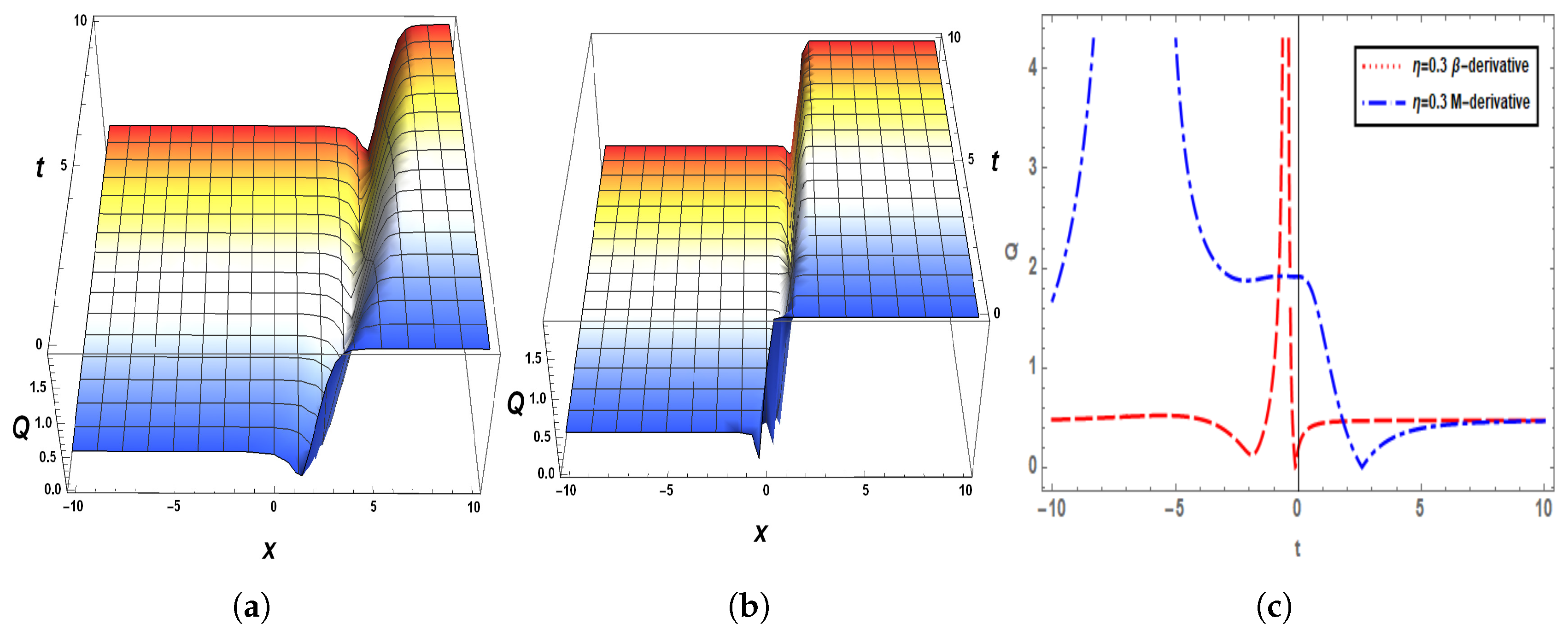
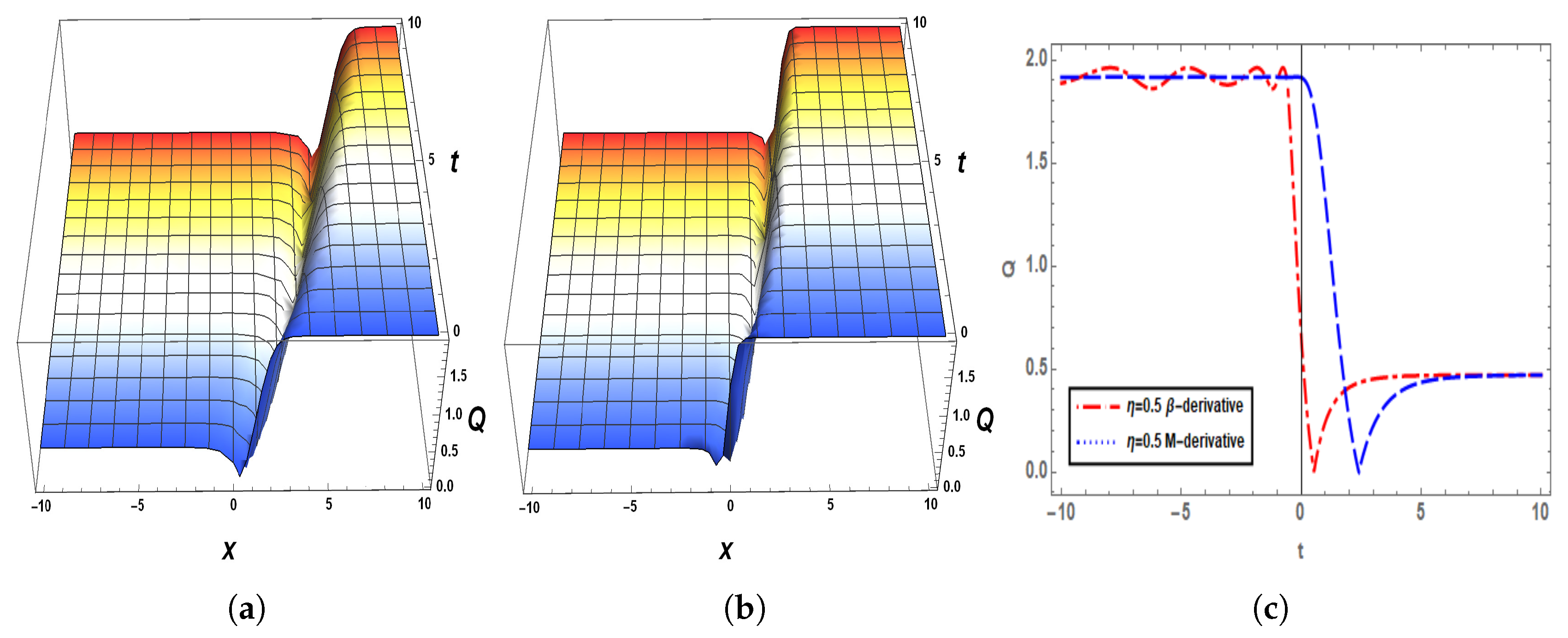
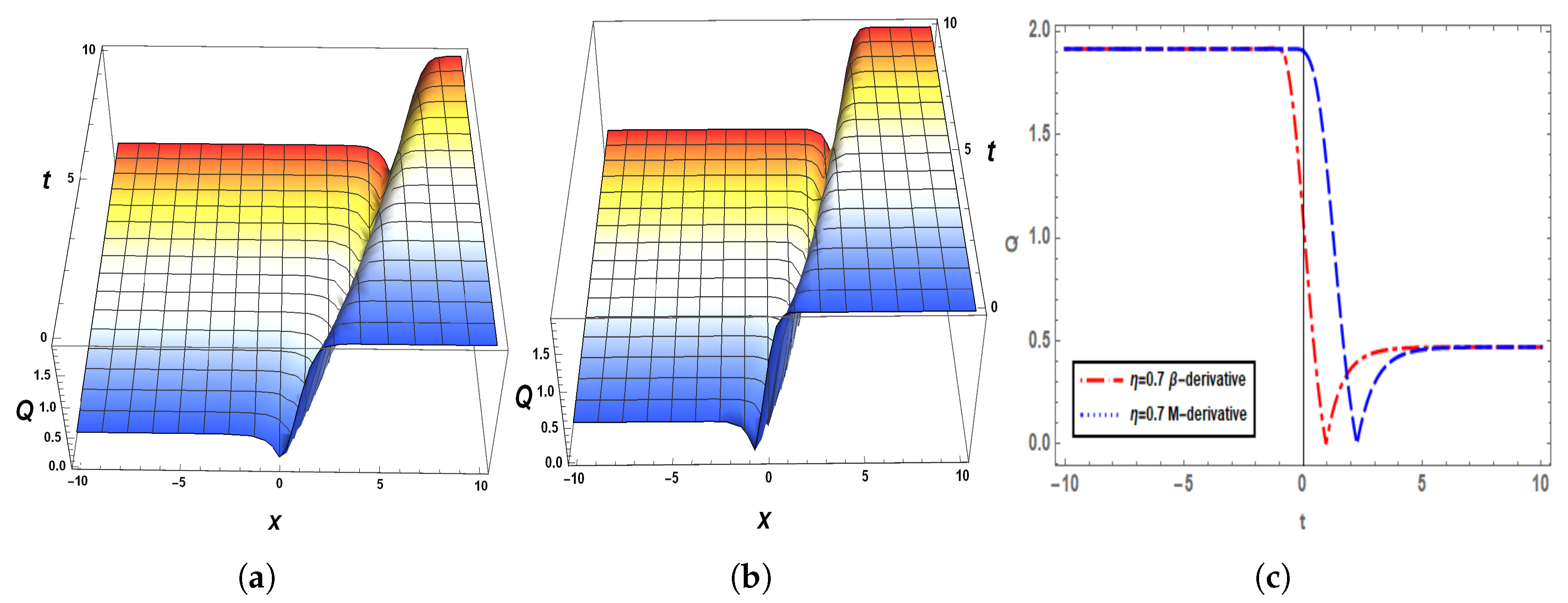
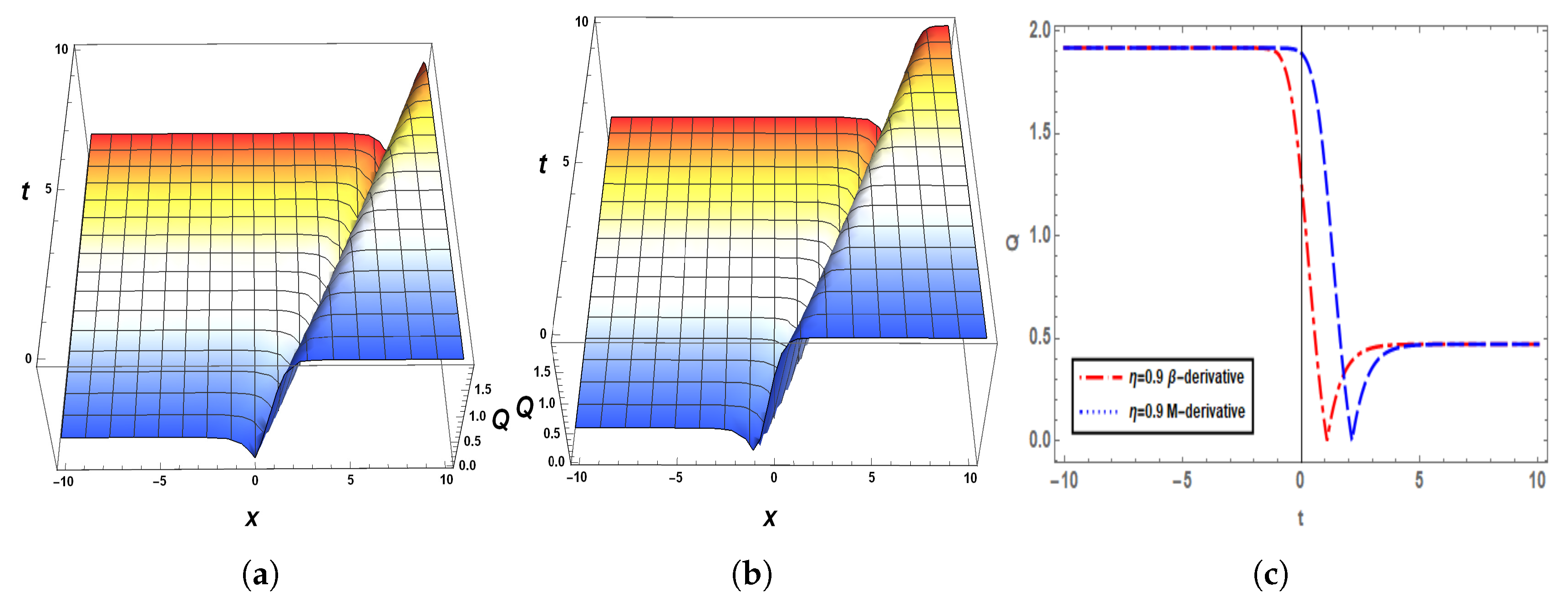
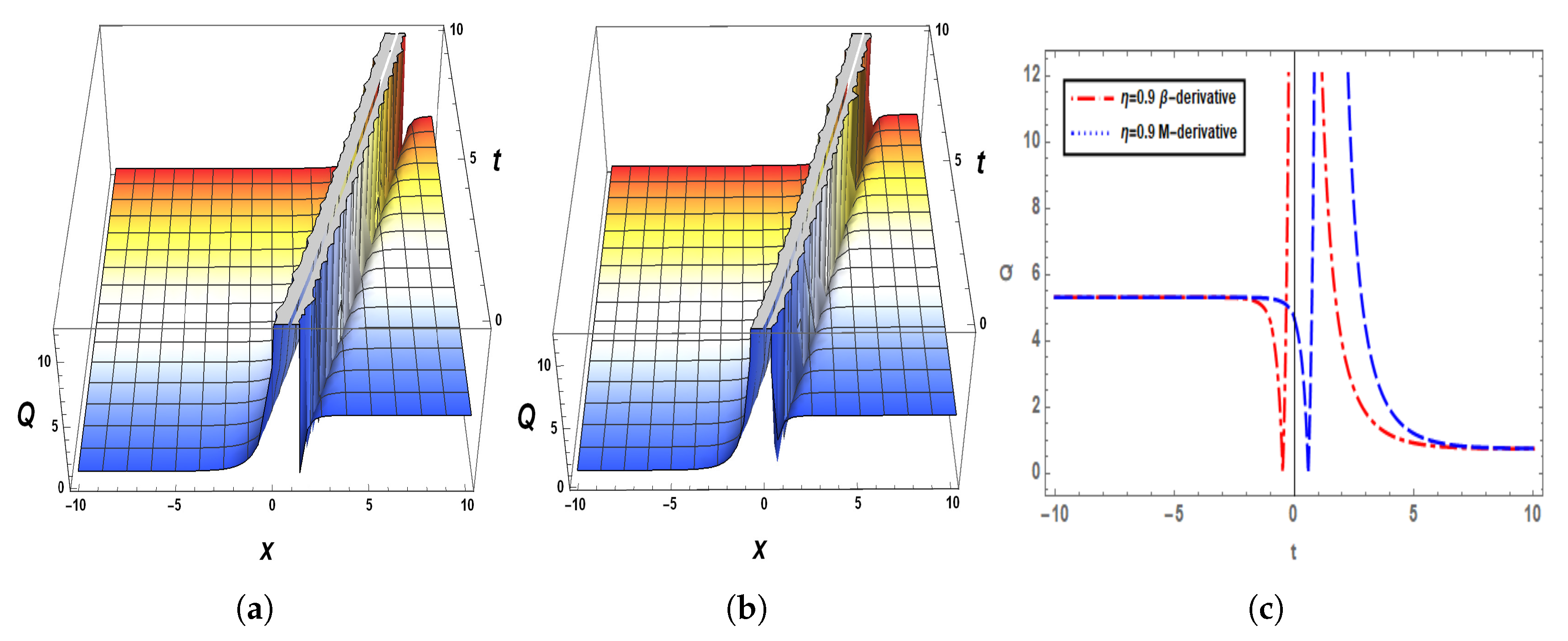
5. Graphical Analysis of the Solutions

This section is devoted to the physical explanation of the graphical presentation and significance of the obtained results.
Figure 1a,b display the 3D Gray-type soliton propagation at fractional order η = 0.3 with the Beta and M-truncated fractional operator, respectively. Figure 1c presents a 2D comparison between the utilized fractional operators and predicting that the solitary wave by the β derivative has less singularity than other solitary waves by the M-truncated derivative having the same amplitude at η = 0.3 .
Similarly, Figure 2, Figure 3 and Figure 4 predict the Gray soliton in 3D and 2D as well, η = 0.5 , 0.7 , 0.9 , respectively. One can observe that, as the fractional order is increasing and coming close to the classical order, the singularity vanishes. More clearly, Figure 5a,b present the influence of the fractional order on the propagation of the soliton. Figure 5c depicts the behavior of the soliton at the integer order. It is observed that the classical derivative is unable to express the behavior as the fractional operators are describing. The fractional operators predict that the solution contains a singularity at η 0.3 . The validity and accuracy of these fractional operators can be ensured as the fractional propagating behavior of the solution is tending to the behavior of the integer-order soliton solution as the fractional order is increasing.
Figure 6a,b display the 3D combined bright–dark-type soliton propagation at fractional order η = 0.3 with the Beta and M-truncated fractional operator, respectively. Figure 6c presents the 2D comparison between the utilized fractional operators and predicting that the solitary wave by the β derivative has less singularity than other solitary waves by the M-truncated derivative having the same amplitude at η = 0.3 .
Similarly, Figure 7, Figure 8 and Figure 9 predict the combined bright–dark soliton in 3D and 2D as well, η = 0.5 , 0.7 , 0.9 , respectively. More clearly, Figure 10a,b present the influence of the fractional order on the propagation of the soliton. Figure 10c depicts the behavior of the soliton at integer order. It is observed that the classical derivative is unable to express the behavior as the fractional operators are describing. The amplitude of the solitary wave at the fractional order is greater than the amplitude of the solitary wave at integer order. The validity and accuracy of these fractional operators can be ensured as the fractional propagating behavior of the solution is tending to the behavior of the integer-order soliton solution as the fractional order is increasing.

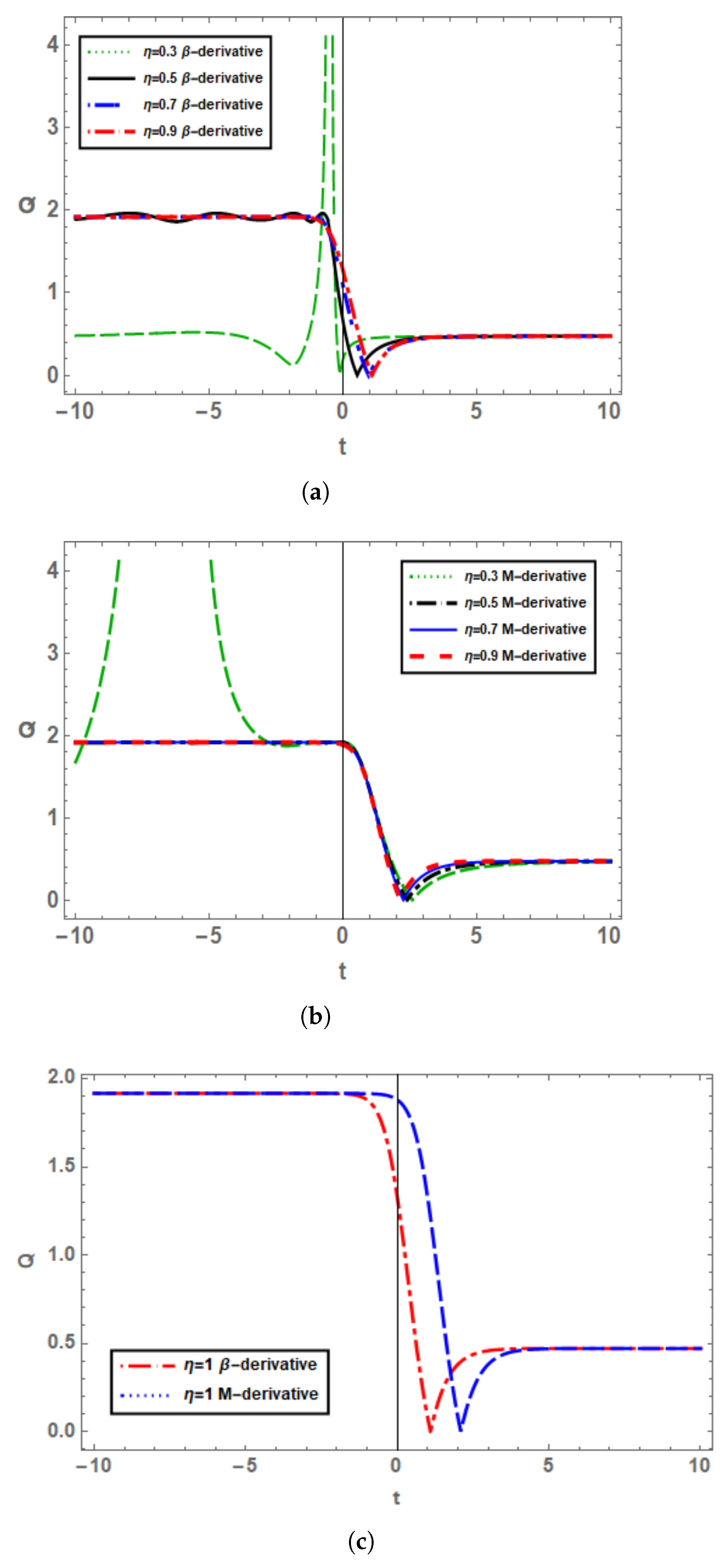
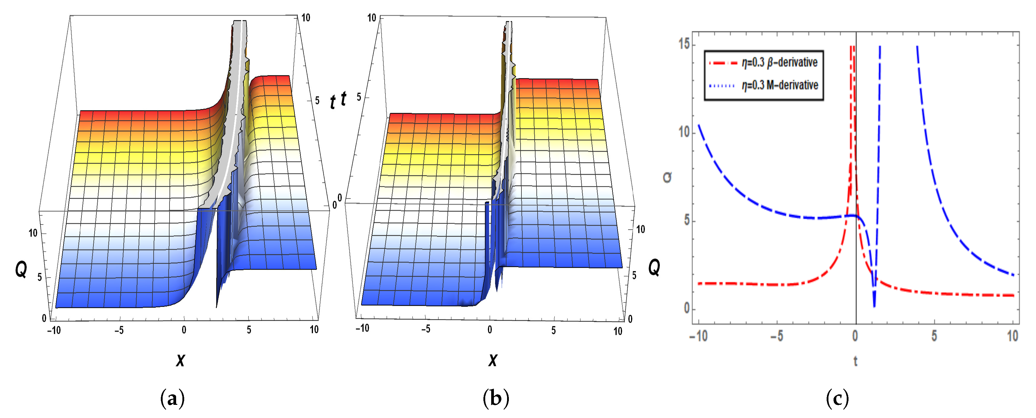
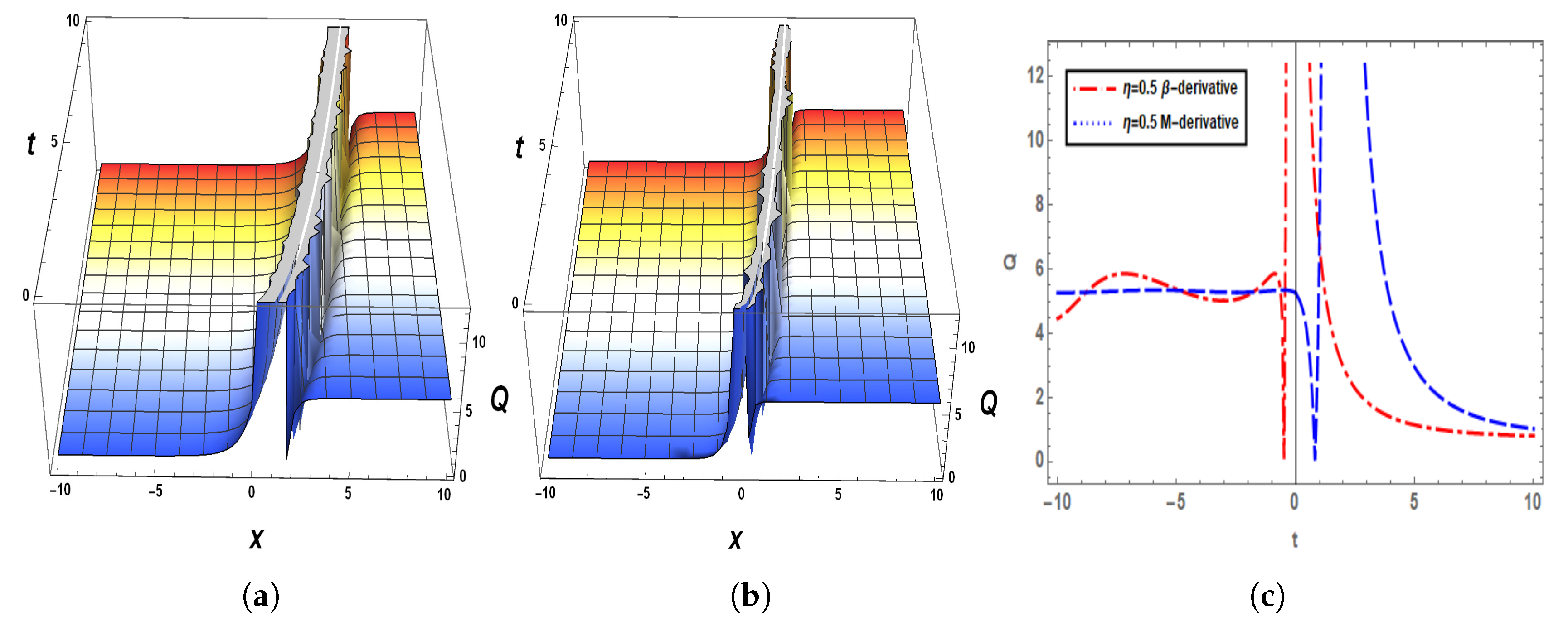
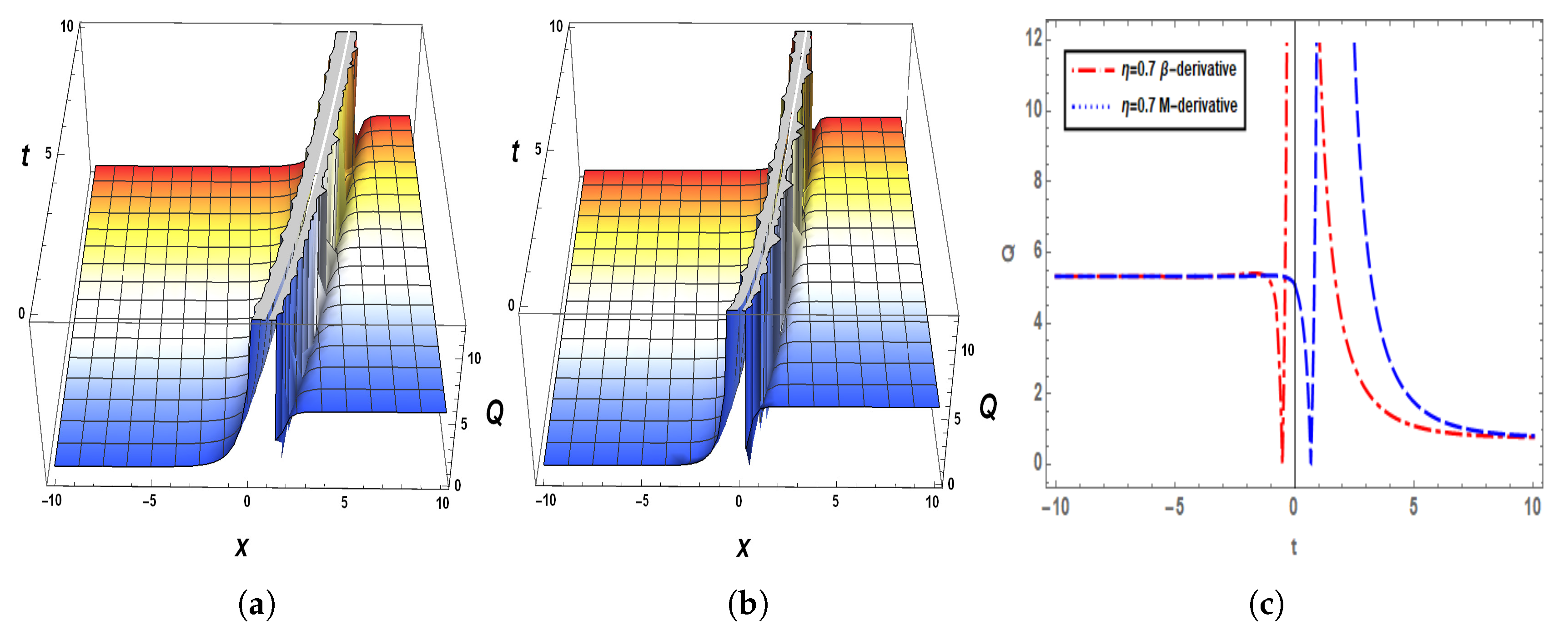
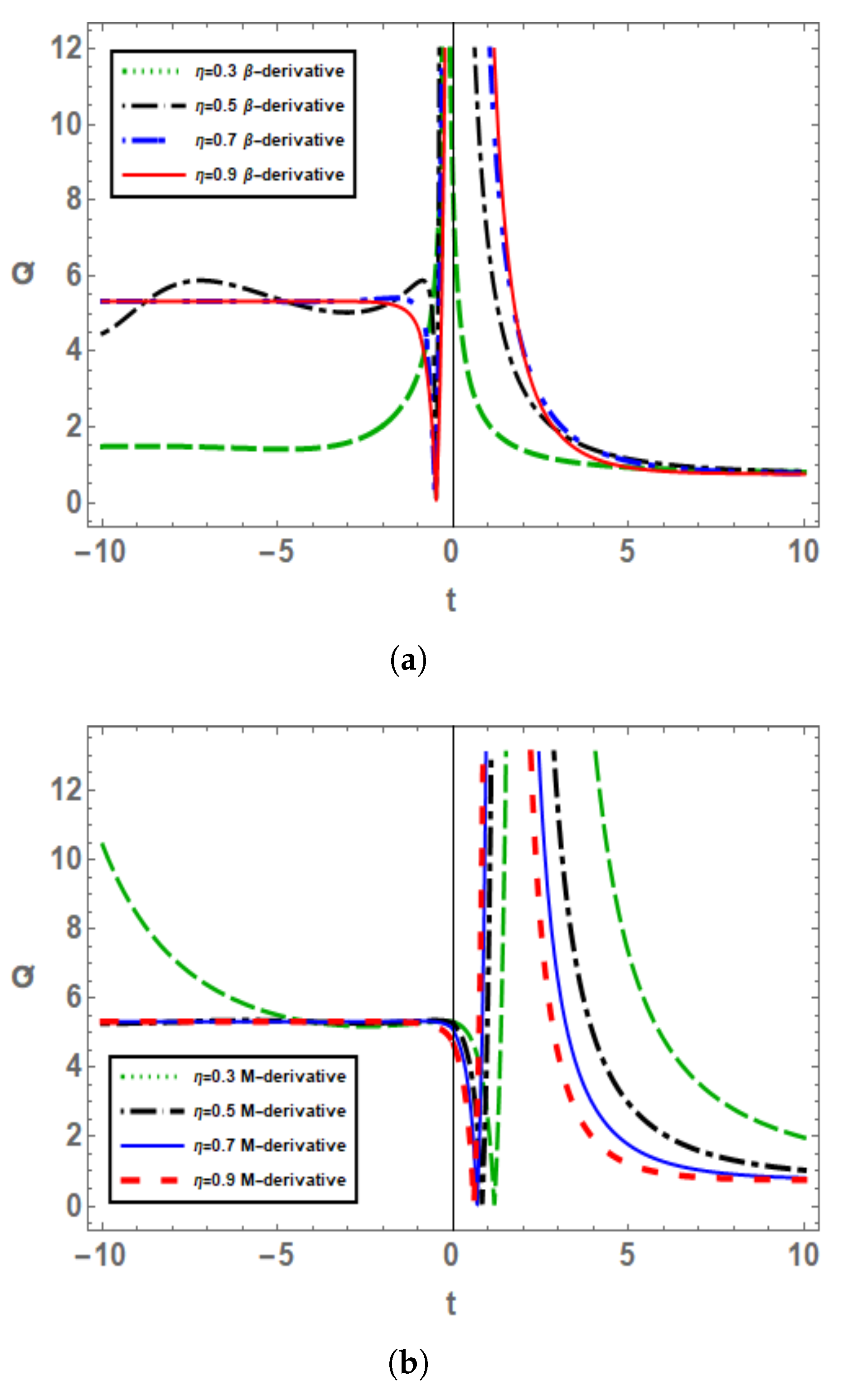
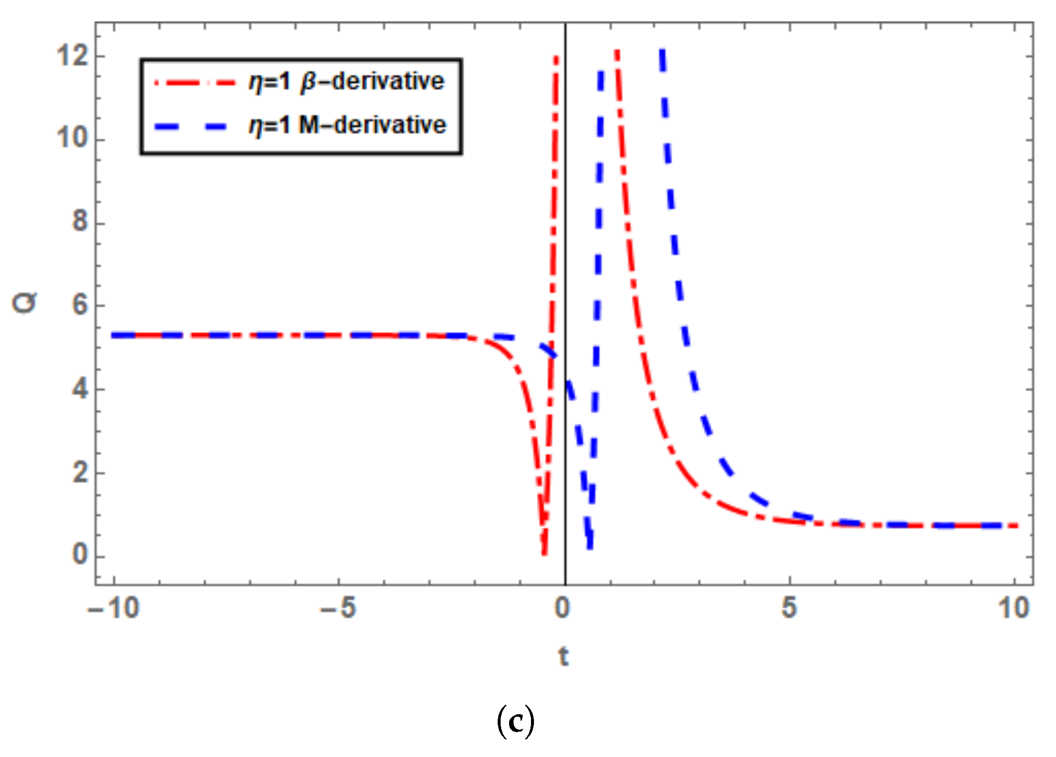
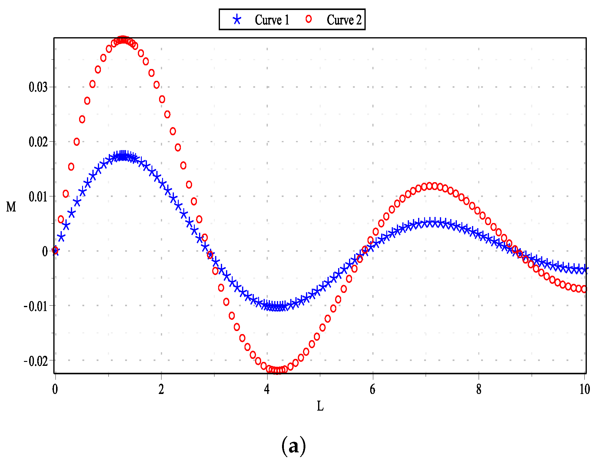
6. Sensitivity Analysis

This section describes the proposed system’s sensitive behavior. The sensitivity method is a tool to analyzing how many variations in the input parameters for a specific variable will affect the results of a mathematical model. Sensitivity analysis can be used in a variety of fields, including investment, business analysis, engineering, environmental studies, physics, and chemistry. Sensitivity analysis is used to analyze the influence of uncertainty on the output of the model. Sensitivity analysis investigates how different values of an independent variable affect a certain dependent variable under a given set of assumptions. Below is a description of the given system (see Figure 11):

7. Conclusions

This paper discussed the soliton and soliton-like structures in the fractional regularized long-wave equation. A variety of these structures were retrieved using the NAEM. The Beta and M-truncated derivatives were introduced to solve the fractional RLW equation, which had not yet been solved by the NAEM. There are twelve different cases in these solutions. The constraint conditions, which are also listed beside the solutions, guarantee the existence of solutions derived from these functions. The bright, dark, singular soliton, as well as the bright–dark soliton solutions were retrieved. Furthermore, our findings showed that the method we used is extremely simple, convenient, and effective for extracting optical solitons from fractional RLW equations and other models that will be studied in the future. Scientists need to have the resulting soliton solutions to agree on the physical event of this equation. The behaviors of various solutions have been visualized using 3 D and 2 D graphics by selecting appropriate parameter values. The method described here is useful for exploring the multiple challenges found in science and engineering. Lastly, the sensitivity analysis of the system was performed and depicted through graphs thoroughly.

8. Future Work

In this work, we discovered the soliton solutions of Equation (32) using the Beta and M-truncated fractional derivatives on the RLW equation. In addition, we may develop further derivatives on the same platform in the future in various formats. We may analyze the graphical behavior of soliton solutions that provide the same outcomes as we found when using conformable fractional derivatives by employing these different types of derivatives. Moreover, multiple solitons, rogue waves, breathers, bifurcation analysis, chaos analysis, and modulational instability gain spectrum visualization can be studied and explored.

Author Contributions

Formal analysis, problem formulation, investigation, methodology: W.A.F.; supervision, funding, resources: A.T. and M.A.E.-R.; validation, graphical discussion, software: R.U.R. and W.A.F.; review and editing: R.M., E.A.A.-Z. and M.A.E.-R. All authors have read and agreed to the published version of the manuscript.

Funding

King Khalid University, Abha, Saudi Arabia, for funding this work through the Large Groups Project under Grant Number RGP. 2/73/43.

Informed Consent Statement

Not applicable.

Data Availability Statement

All the data are within the manuscript.

Acknowledgments

Magda Abd El-Rahman extends appreciation to the Deanship of Scientific Research at King Khalid University, Abha, Saudi Arabia.

Conflicts of Interest

The authors declare that they have no competing interests.

References

  1. Yusuf, A.; Sulaiman, T.A.; Mirzazadeh, M.; Hosseini, K. M-truncated optical solitons to a nonlinear Schrödinger equation describing the pulse propagation through a two-mode optical fiber. Opt. Quantum Electron. 2021, 53, 1–17. [Google Scholar] [CrossRef]
  2. Alabedalhadi, M.; Al-Smadi, M.; Al-Omari, S.; Karaca, Y.; Momani, S. New Bright and Kink Soliton Solutions for Fractional Complex Ginzburg–Landau Equation with Non-Local Nonlinearity Term. Fractal Fract. 2022, 6, 724. [Google Scholar] [CrossRef]
  3. Az-Zo’bi, E.A. Peakon and solitary wave solutions for the modified Fornberg-Whitham equation using the simplest equation method. Int. J. Math. Comput. Sci. 2019, 14, 635–645. [Google Scholar]
  4. Sarwar, S.; Furati, K.; Arshad, M. Abundant wave solutions of conformable space-time fractional order fokas wave model arising in physical sciences. Alex. Eng. J. 2021, 60, 2687–2696. [Google Scholar] [CrossRef]
  5. Khodadad, F.S.; M-Alizamini, S.M.; Günay, B.; Akinyemi, L.; Rezazadeh, H.; Inc, M. Abundant optical solitons to the Sasa-Satsuma higher-order nonlinear Schrödinger equation. Opt. Quantum Electron. 2021, 53, 702. [Google Scholar] [CrossRef]
  6. Ullah, N.; Asjad, M.I.; Awrejcewicz, J.; Muhammad, T.; Baleanu, D. On soliton solutions of the fractional-order nonlinear model appears in physical sciences. AIMS Math. 2022, 7, 7421–7440. [Google Scholar] [CrossRef]
  7. Darvishi, M.T.; Najafi, M.; Wazwaz, A.M. Conformable space-time fractional nonlinear (1+1)-dimensional Schrödinger-type models and their traveling wave solutions. Chaos Solitons Fractals 2021, 150, 111187. [Google Scholar] [CrossRef]
  8. Asghar, U.; Faridi, W.A.; Asjad, M.I.; Eldin, S.M. The Enhancement of Energy-Carrying Capacity in Liquid with Gas Bubbles, in Terms of Solitons. Symmetry 2022, 14, 2294. [Google Scholar] [CrossRef]
  9. Korpinar, Z.; Tchier, F.; Inç, M.; Ragoub, L.; Bayram, M. New soliton solutions of the fractional Regularized Long Wave Burgers equation by means of conformable derivative. Results Phys. 2019, 14, 102395. [Google Scholar] [CrossRef]
  10. Wazwaz, A.M. Bright and dark optical solitons of the (2+1)-dimensional perturbed nonlinear Schrödinger equation in nonlinear optical fibers. Opt. Int. J. Light Electron Opt. 2021, 251, 168334. [Google Scholar] [CrossRef]
  11. Ding, C.C.; Gao, Y.T.; Deng, G.F.; Wang, D. Lax pair, conservation laws, Darboux transformation, breathers, and rogue waves for the coupled nonautonomous nonlinear SchrÖdinger system in an inhomogeneous plasma. Chaos Solitons Fractal 2020, 133, 109580. [Google Scholar] [CrossRef]
  12. Raza, N.; Jhangeer, A.; Rahman, R.U.; Butt, A.R.; Chu, Y.M. Sensitive visualization of the fractional Wazwaz-Benjamin-Bona-Mahony equation with fractional derivatives: A comparative analysis. Results Phys. 2021, 25, 104171. [Google Scholar] [CrossRef]
  13. Tariq, K.U.; Younis, M.; Rizvi, S.T.R.; Bulut, H. M-truncated fractional optical solitons and other periodic wave structures with Schrödinger-Hirota equation. Mod. Phys. Lett. B 2020, 34, 2050427. [Google Scholar] [CrossRef]
  14. Arshed, S.; Rahman, R.U.; Raza, N.; Khan, A.K.; Inc, M. A variety of fractional soliton solutions for three important coupled models arising in mathematical physics. Int. J. Mod. Phys. B 2021, 36, 2250002. [Google Scholar] [CrossRef]
  15. Cinar, M.; Secer, A.; Bayram, M. On the optical soliton solutions of time-fractional Biswas–Arshed equation including the beta or M-truncated derivatives. Opt. Quantum Electron. 2023, 55, 186. [Google Scholar] [CrossRef]
  16. Mohammed, W.W.; Al-Askar, F.M.; Cesarano, C.; El-Morshedy, M. Solitary Wave Solutions of the Fractional-Stochastic Quantum Zakharov–Kuznetsov Equation Arises in Quantum Magneto Plasma. Mathematics 2023, 11, 488. [Google Scholar] [CrossRef]
  17. Ismael, F.H.; Bulut, H.; Baskonus, H.M.; Gao, W. Dynamical behaviors to the coupled Schrödinger-Boussinesq system with the beta derivative. AIMS Math. 2021, 6, 7909–7928. [Google Scholar] [CrossRef]
  18. Zulqarnain, R.M.; Ma, W.X.; Eldin, S.M.; Mehdi, K.B.; Faridi, W.A. New Explicit Propagating Solitary Waves Formation and Sensitive Visualization of the Dynamical System. Fractal Fract. 2023, 7, 71. [Google Scholar] [CrossRef]
  19. Ali, H.S.; Habib, M.A.; Miah, M.M.; Akbar, M.A. Solitary wave solutions to some nonlinear fractional evolution equations in mathematical physics. Heliyon 2020, 6, e03727. [Google Scholar] [CrossRef]
  20. Kumar, S.; Niwas, M.; Osman, M.S.; Abdou, M. Abundant different types of exact-soliton solutions to the (4+1)-dimensional Fokas and (2+1)-dimensional Breaking soliton equations. Commun. Theor. Phys. 2021, 73, 105007. [Google Scholar] [CrossRef]
  21. Esen, H.; Ozdemir, N.; Secer, A.; Bayram, M.; Sulaiman, T.A.; Yusuf, A. Solitary wave solutions of chiral nonlinear Schrödinger equations. Mod. Phys. Lett. B 2021, 35, 2150472. [Google Scholar] [CrossRef]
  22. Bekir, A.; Cevikel, A.C. New exact traveling wave solutions of nonlinear physical models. Chaos Solitons Fractals 2009, 41, 1733–1739. [Google Scholar] [CrossRef]
  23. Cinar, M.; Onder, I.; Secer, A.; Sulaiman, T.A.; Yusuf, A.; Bayram, M. Optical solitons of the (2+1)-dimensional Biswas–Milovic equation using modified extended tanh-function method. Optik 2021, 245, 167631. [Google Scholar] [CrossRef]
  24. Nadeem, M.; Jafari, H.; Akgül, A.; De la Sen, M. A Computational Scheme for the Numerical Results of Time-Fractional Degasperis–Procesi and Camassa–Holm Models. Symmetry 2022, 14, 2532. [Google Scholar] [CrossRef]
  25. Khan, A.; Ali, A.; Ahmad, S.; Saifullah, S.; Nonlaopon, K.; Akgül, A. Nonlinear Schrödinger equation under non-singular fractional operators: A computational study. Results Phys. 2022, 43, 106062. [Google Scholar] [CrossRef]
  26. Qureshi, Z.A.; Bilal, S.; Khan, U.; Akgül, A.; Sultana, M.; Botmart, T.; Zahran, H.Y.; Yahia, I.S. Mathematical analysis about the influence of Lorentz force and interfacial nanolayers on nanofluids flow through orthogonal porous surfaces with the injection of SWCNTs. Alex. Eng. J. 2022, 61, 12925–12941. [Google Scholar] [CrossRef]
  27. Xu, C.; Liu, Z.; Pang, Y.; Akgül, A.; Baleanu, D. Dynamics of HIV-TB coinfection model using classical and Caputo piecewise operator: A dynamic approach with real data from South-East Asia, European and American regions. Chaos Solitons Fractals 2022, 165, 112879. [Google Scholar] [CrossRef]
  28. Wazwaz, A.M.; Alhejaili, W.; AL-Ghamdi, A.O.; El-Tantawy, S.A. Bright and dark modulated optical solitons for a (2+1)-dimensional optical Schrödinger system with third-order dispersion and nonlinearity. Optik 2023, 274, 170582. [Google Scholar] [CrossRef]
  29. Hussain, A.; Bano, S.; Khan, I.; Baleanu, D.; Nisar, K.S. Lie Symmetry Analysis, Explicit solutions and conservation laws of a spatially two-dimensional Burgers Huxley equation. Symmetry 2020, 12, 170. [Google Scholar] [CrossRef]
  30. Yang, X.; Zhang, Z.; Wazwaz, A.M.; Wang, Z. A direct method for generating rogue wave solutions to the (3+1)-dimensional Korteweg-de Vries Benjamin-Bona-Mahony equation. Phys. Lett. A 2022, 449, 128355. [Google Scholar] [CrossRef]
  31. Akinyemi, L.; Mirzazadeh, M.; Hosseini, K. Solitons and other solutions of perturbed nonlinear Biswas–Milovic equation with Kudryashov’s law of refractive index. Nonlinear Anal. Model. Control 2022, 27, 1–7. [Google Scholar] [CrossRef]
  32. Wang, K.J. Variational principle and diverse wave structures of the modified Benjamin-Bona-Mahony equation arising in the optical illusions field. Axioms 2022, 11, 445. [Google Scholar] [CrossRef]
  33. Liu, J.G.; Yang, X.J.; Geng, L.L.; Yu, X.J. On fractional symmetry group scheme to the higher-dimensional space and time fractional dissipative Burgers equation. Int. J. Geom. Methods Mod. Phys. 2022, 19, 2250173–2251483. [Google Scholar] [CrossRef]
  34. Akbar, M.A.; Wazwaz, A.M.; Mahmud, F.; Baleanu, D.; Roy, R.; Barman, H.K.; Mahmoud, W.; Al Sharif, M.A.; Osman, M.S. Dynamical behavior of solitons of the perturbed nonlinear SchrÖdinger equation and microtubules through the generalized Kudryashov scheme. Results Phys. 2022, 43, 106079. [Google Scholar] [CrossRef]
  35. Siddique, I.; Jaradat, M.M.; Zafar, A.; Mehdi, K.B.; Osman, M.S. Exact traveling wave solutions for two prolific conformable M-Fractional differential equations via three diverse approaches. Results Phys. 2021, 28, 104557. [Google Scholar] [CrossRef]
  36. Ghayad, M.S.; Badra, N.M.; Ahmed, H.M.; Rabie, W.B. Derivation of optical solitons and other solutions for nonlinear Schrödinger equation using modified extended direct algebraic method. Alex. Eng. J. 2023, 64, 801–811. [Google Scholar] [CrossRef]
  37. Ghanbari, B.; Baleanu, D. Applications of two novel techniques in finding optical soliton solutions of modified nonlinear Schrödinger equations. Results Phys. 2023, 44, 106171. [Google Scholar] [CrossRef]
  38. Sarhan, A.; Burqan, A.; Saadeh, R.; Al-Zhour, Z. Analytical Solutions of the Nonlinear Time-Fractional Coupled Boussinesq-Burgers Equations Using Laplace Residual Power Series Technique. Fractal Fract. 2022, 6, 631. [Google Scholar] [CrossRef]
  39. Rezazadeh, H.; Inc, M.; Baleanu, D. New solitary wave solutions for variants of (3+1)-dimensional Wazwaz-Benjamin-Bona-Mahony equations. Front. Phys. 2020, 8, 332. [Google Scholar] [CrossRef]
  40. Arshed, S.; Raza, N.; Butt, A.R.; Akgül, A. Exact solutions for Kraenkel-Manna-Merle model in saturated ferromagnetic materials using Beta-derivative. Phys. Scr. 2021, 96, 124018. [Google Scholar] [CrossRef]
  41. Riaz, M.B.; Jhangeer, A.; Awrejcewicz, J.; Baleanu, D.; Tahir, S. Fractional propagation of short light pulses in monomode optical fibers: Comparison of beta derivative and truncated M-fractional derivative. J. Comput. Nonlinear Dyn. 2022, 17, 031002. [Google Scholar] [CrossRef]
  42. Sousa, J.C.; Oliveira, E.C. A New Truncated M-Fractional Derivative Type Unifying Some Fractional Derivative Types with Classical Properties. Int. J. Anal. Appl. 2018, 16, 83–96. [Google Scholar]
Figure 1. Depiction of 3 D and 2 D graphs of Q 4 , 1 ( x , t ) for μ = 0.1 , γ = 0.1 , σ = 2 , θ = 0.5 , ϑ = 1 , ϵ = 2 , C = 1 , and λ = 1 . Here, (a,b) display the 3 D graphs with Beta and M-truncated derivatives, while (c) represents the 2 D surface taking η = 0.3 at t = 1 .
Fractalfract 07 00136 g001
Figure 2. For Q 4 , 1 ( x , t ) , we take μ = 0.1 , γ = 0.1 , σ = 2 , θ = 0.5 , ϑ = 1 , ϵ = 2 , C = 1 , and λ = 1 . (ac) reflect the 3 D and 2 D graphs employing η = 0.5 at t = 1 .
Fractalfract 07 00136 g002
Figure 3. For Q 4 , 1 ( x , t ) , we take μ = 0.1 , γ = 0.1 , σ = 2 , θ = 0.5 , ϑ = 1 , ϵ = 2 , C = 1 , and λ = 1 . Here, (ac) show the 3 D , as well as 2 D graphics letting η = 0.7 .
Fractalfract 07 00136 g003
Figure 4. Here, (ac) manifest the 3 D and 2 D plots for Q 4 , 1 ( x , t ) taking η = 0.9 at t = 1 .
Fractalfract 07 00136 g004
Figure 5. The 2 D plots of Q 4 , 1 ( x , t ) for both operators taking μ = 0.5 , γ = 0.5 , σ = 1.1 , and ω = 1 at t = 1 with different values of fractional parameter η .
Fractalfract 07 00136 g005
Figure 6. For Q 8 , 2 ( x , t ) , now take μ = 0.5 , γ = 0.8 , σ = 0 , θ = 1 , ϑ = 1 , ϵ = 0.5 , λ = 1 and C = 1 . Here, (ac) represent 3 D and 2 D graphs with both operators letting η = 0.3 .
Fractalfract 07 00136 g006
Figure 7. For Q 8 , 2 ( x , t ) , we consider μ = 0.5 , γ = 0.8 , σ = 0 , θ = 1 , ϑ = 1 , ϵ = 0.5 , λ = 1 , and C = 1 . (ac) show 3 D , as well as the 2 D plots with Beta and M-truncated derivatives for η = 0.5 .
Fractalfract 07 00136 g007
Figure 8. Graphical depiction of Q 8 , 2 ( x , t ) taking μ = 0.5 , γ = 0.8 , σ = 0 , θ = 1 , ϑ = 1 , ϵ = 0.5 , λ = 1 , and C = 1 . (ac) reflect 3 D and 2 D profiles with Beta and M-truncated operators for η = 0.7 .
Fractalfract 07 00136 g008
Figure 9. Graphical representation of Q 8 , 2 ( x , t ) letting μ = 0.5 , γ = 0.8 , σ = 0 , θ = 1 , ϑ = 1 , ϵ = 0.5 , λ = 1 , and C = 1 . Here, (ac) show 3 D , as well as the 2 D surface graphs for η = 0.9 .
Fractalfract 07 00136 g009
Figure 10. The 2 D profiles of Q 8 , 2 ( x , t ) for M-truncated and Beta operators with μ = 0.5 , γ = 0.8 , σ = 0 , θ = 1 , ϑ = 1 , ϵ = 0.5 , λ = 1 , and C = 1 at t = 1 .
Fractalfract 07 00136 g010aFractalfract 07 00136 g010b
Figure 11. (a) reflects the analysis of the system letting the initial conditions ( u , v ) = ( 0.0 , 0.055 ) and ( u , v ) = ( 0.0 , 0.025 ) with ϵ = 0.1 , δ = 0.1 , ν = 2.5 , θ = 1 , and C = 0.001 . It is indeed important to see that overlapping can be observed between the curves. (b) Here, we take the initial conditions ( u , v ) = ( 0.01 , 0.055 ) , the results of which are shown by the red curve and those of ( u , v ) = ( 0.012 , 0.045 ) represented by the blue color.
Fractalfract 07 00136 g011aFractalfract 07 00136 g011b
Disclaimer/Publisher’s Note: The statements, opinions and data contained in all publications are solely those of the individual author(s) and contributor(s) and not of MDPI and/or the editor(s). MDPI and/or the editor(s) disclaim responsibility for any injury to people or property resulting from any ideas, methods, instructions or products referred to in the content.

