Article

The First Integral of the Dissipative Nonlinear Schrödinger Equation with Nucci’s Direct Method and Explicit Wave Profile Formation

1
Department of Mathematics, University of Management and Technology, Lahore 54770, Pakistan
2
Mathematics Department, College of Science, University of Bisha, P.O. Box 344, Bisha 61922, Saudi Arabia
3
Department of Physics, College of Science, King Khalid University, Abha 61413, Saudi Arabia
4
Department of Radiation Physics, National Center of Radiation Research and Technology (NCRRT), Atomic Energy Authority, Cairo 11787, Egypt
5
Applied Mathematical Physics Research Group, Physics Department, Faculty of Science, Mansoura University, Mansoura 35516, Egypt
6
Higher Institute of Engineering and Technology, New Damietta 34517, Egypt
*
Authors to whom correspondence should be addressed.
Fractal Fract. 2023, 7(1), 38; https://doi.org/10.3390/fractalfract7010038
Submission received: 9 December 2022 / Revised: 24 December 2022 / Accepted: 27 December 2022 / Published: 29 December 2022
(This article belongs to the Special Issue Feature Papers for Numerical and Computational Methods Section)

Abstract

:
The propagation of optical soliton profiles in plasma physics and atomic structures is represented by the ( 1 + 1 ) dimensional Schrödinger dynamical equation, which is the subject of this study. New solitary wave profiles are discovered by using Nucci’s scheme and a new extended direct algebraic method. The new extended direct algebraic approach provides an easy and general mechanism for covering 37 solitonic wave solutions, which roughly corresponds to all soliton families, and Nucci’s direct reduction method is used to develop the first integral and the exact solution of partial differential equations. Thus, there are several new solitonic wave patterns that are obtained, including a plane solution, mixed hyperbolic solution, periodic and mixed periodic solutions, a mixed trigonometric solution, a trigonometric solution, a shock solution, a mixed shock singular solution, a mixed singular solution, a complex solitary shock solution, a singular solution, and shock wave solutions. The first integral of the considered model and the exact solution are obtained by utilizing Nucci’s scheme. We present 2-D, 3-D, and contour graphics of the results obtained to illustrate the pulse propagation characteristics while taking suitable values for the parameters involved, and we observed the influence of parameters on solitary waves. It is noticed that the wave number α and the soliton speed μ are responsible for controlling the amplitude and periodicity of the propagating wave solution.

1. Introduction

The Schrödinger equation is one of the fundamental equations in quantum theory. In quantum physics, the Schrödinger equation is frequently employed to determine a wave function’s progression over time. In other words, the primary application of the Schrödinger equation is to the prediction of the trajectory of a particle’s motion, and these findings play a significant role in the advancement of modern physics, as well as applied mathematics [1]. It is also characterized as a classical field equation. One of the applications is the comparison of the propagation of light in a planar waveguide with a nonlinear optical fiber [2,3]. The study of wave theory shows that the the nonlinear Schrödinger equation (NLSE) is a feasible tool for the demonstration of self-monochromatic waves in a dispersive medium. The NLSE is more common in the disciplines of plasma physics, matter physics, Heisenberg spin chains, deep water waves, computer networking, and optical communication (Seadawy et al. [4], Liu et al. [5], and Wang et al. [6]). The dissipative NLSE is extremely helpful for the modeling of amplitude in the study of dispersive and dissipative media. Therefore, the d-NLSE is a viable technique for the modeling of dissipative self-modulating monochromatic waves with dispersion. The estimation of quasi-monochromatic waves’ packets with slow alterations in nonlinear systems is provided by the NLSE’s linear and nonlinear dispersive and dissipative effects (Ma et al. [7]; Mo et al. [8]; Jiang et al. [9]).
Meanwhile, numerous researchers have worked on distinct forms of NLSEs. Chen et al. [10] gave interactions and a general periodic solution of the NLSE. The d-NLSE’s asymptotic behaviors were studied by Cazenave et al. [11]. Keller–Segel dynamics were studied by Lopez with the NLSE [12]. Weng et al. [13] also conducted an asymptotic analysis with some semi-rational vector solutions of the n-component NLSE, and some of the optical solutions were given by Savaissou by using a power law [14]. Seadway found soliton solutions of the Korteweg–de-Vries–Zakharov–Kuznetsov equation [15]. Akram worked on the CGL equation and obtained optical solutions, and they also used the Triki–Biswas equation to study ultrashort pulse propagation in optical fiber frameworks [16,17,18]. Kumar studied higher-order equations, such as the Chaffee–Infante equation, BLMP equation, and rdDym equation, with different approaches [19,20,21]. Imran explored an improved perturbed Schrödinger equation with the use of the Ker law [22] and examined the Chen–Lee–Liu dynamical equation with Nucci’s reduction approach [23]. Adil et al. [24] obtained the traveling wave solution of nonlinear directional couplers and studied fusion and fission reactions with soliton solutions [25]. The bright and dark soliton solutions of the ( 2 + 1 ) NLSE were studied by Wazwaz [26].
The optical solution of the (3 + 1) NLSE was given by Lanre [27]. Kudryashov gave the solutions of periodic and solitary waves by using a reduced form of a higher-order NLSE, and he also vigilantly worked on a resonant NLSE for optical solitons [28,29]. Wang worked on a chiral NLSE and figured out its abundant solutions [30]. Faridi et al. [31] analyzed the isotropic bi-quadratic Heisenberg spin chain phenomenon and found soliton solutions, and they also analyzed propagating wave structures of cold bosonic atoms and obtain soliton solutions [32]. Tahir worked on different models and found their soliton solution with the help of updated techniques [33,34,35]. In parallel to this, there are multiple researchers who have worked on different linear and nonlinear equations, such as Akgül [36], who worked on the nonlinear stochastic Newell–Whitehead–Segel equation, an HIV/AIDS model [37], pseudo-parabolic differential equations [38], the fractal–fractional Klein–Gordon equation [39], and the kernel Hilbert space method [40]. Cubic–quintic nonlinear Schrödinger equations were also studied by Fabio [41], and he obtained the dark and bright solutions of the nonlinear Schrödinger equation [42], etc.
The considered model was studied by Seadawy. He produced the bright and dark soliton solutions by using ansatz function methods [43]. To obtain the soliton solutions in the current work, a novel direct extended algebraic method is applied to the model.
In the present study, Section 2 presents the model and its structure. Section 3 portrays a detailed description of the proposed technique and solutions of the model with graphs of the solutions. A graphical discussion is included in Section 4. At the end, Section 5 contains the summary as a conclusion.

2. Description of the Model

We consider the dissipative NLSEs
i U t + 1 2 U x x + U U 2 = 0 , i = 1 ,
and
i U t 1 2 U x x + U U 2 = 0 , i = 1 .
The ( 1 + 1 ) dNLSE is [43],
i U t ( x , t ) + a U x x ( x , t ) + b U ( x , t ) 2 U ( x , t ) + i c U ( x , t ) = 0 , i = 1 ,
where the dispersion is represented by a, b is a non-linearity constant, and the dissipative effects are shown by c. If the dissipative effect is weak, c = 0 . This effect can also be shown for various forms of signs of a b < 0 and a b > 0 . The exact localized traveling wave solutions can be generated for the NLSE [43]. There are also some chances of significant modification of the pulse shape if the absorption is reduced and the nonlinear term is made comparable to the dispersion term. The shape of the stationary solution is affected by the sign of a. In fact, if both a > 0 and b > 0, then one can determine the group of exact solutions, which are localized and stationary.

3. Computation of Soliton Solutions

3.1. Description of the Method

Assume a general NPDE of the type:
Y ( U , U t , U x , U t t , U x x , ) = 0 ,
which can be transformed:
M ( R , R , R , ) = 0 ,
by using the following transformation:
U ( x , t ) = U ( κ ) e i Φ ,
where κ = k 1 x + k 2 t and Φ = k 3 x + k 4 t , where the prime sign represents the order of differentiation for different attributes in Equation (5). Assume that Equation (5) has a solution of the form:
U ( κ ) = r = 0 j a r ( P ( κ ) ) r ,
where
P ( κ ) = ln ( ρ ) φ + υ P ( κ ) + ς ( P ( κ ) ) 2 , ρ 0 , 1 .
In addition, ς , υ , and φ are real constants. The general forms of the solutions of Equation (8) w.r.t the real parameters ς , υ , and φ are as follows:
  • For υ 2 4 φ ς < 0 and ς 0 ,
    P 1 ( κ ) = υ 2 ς + 2 ς tan ρ 2 κ ,
    P 2 ( κ ) = υ 2 ς 2 ς cot ρ 2 κ ,
    P 3 ( κ ) = υ 2 ς + 2 ς tan ρ κ ± m n sec ρ κ ,
    P 4 ( κ ) = υ 2 ς + 2 ς cot ρ κ ± m n csc ρ κ ,
    P 5 ( κ ) = υ 2 ς + 4 ς tan ρ 4 κ cot ρ 4 κ .
  • For υ 2 4 φ ς > 0 and ς 0 ,
    P 6 ( κ ) = υ 2 ς 2 ς tanh ρ 2 κ ,
    P 7 ( κ ) = υ 2 ς 2 ς coth ρ 2 κ ,
    P 8 ( κ ) = υ 2 ς + 2 ς tanh ρ κ ± i m n ρ κ ,
    P 9 ( κ ) = υ 2 ς + 2 ς coth ρ κ ± m n ρ κ ,
    P 10 ( κ ) = υ 2 ς 4 ς tanh ρ 4 κ + coth ρ 4 κ .
  • For φ ς > 0 and υ = 0 ,
    P 11 ( κ ) = φ ς tan ρ φ ς κ ,
    P 12 ( κ ) = φ ς cot ρ φ ς κ ,
    P 13 ( κ ) = φ ς tan ρ 2 φ ς κ ± m n sec ρ 2 φ ς κ ,
    P 14 ( κ ) = φ ς cot ρ 2 φ ς κ ± m n csc ρ 2 φ ς κ ,
    P 15 ( κ ) = 1 2 φ ς tan ρ φ ς 2 κ cot ρ φ ς 2 κ .
  • For φ ς < 0 and υ = 0 ,
    P 16 ( κ ) = φ ς tanh ρ φ ς κ ,
    P 17 ( κ ) = φ ς coth ρ φ ς κ ,
    P 18 ( κ ) = φ ς tanh ρ 2 φ ς κ ± i m n ρ 2 φ ς κ ,
    P 19 ( κ ) = φ ς coth ρ 2 φ ς κ ± m n ρ 2 φ ς κ ,
    P 20 ( κ ) = 1 2 φ ς tanh ρ φ ς 2 κ + coth ρ φ ς 2 κ .
  • For υ = 0 and φ = ς ,
    P 21 ( κ ) = tan ρ φ κ ,
    P 22 ( κ ) = cot ρ φ κ ,
    P 23 ( κ ) = tan ρ 2 φ κ ± m n sec ρ 2 φ κ ,
    P 24 ( κ ) = cot ρ 2 φ κ ± m n csc ρ 2 φ κ ,
    P 25 ( κ ) = 1 2 tan ρ φ 2 κ cot ρ φ 2 κ .
  • For υ = 0 and ς = φ ,
    P 26 ( κ ) = tanh ρ φ κ ,
    P 27 ( κ ) = coth ρ φ κ ,
    P 28 ( κ ) = tanh ρ 2 φ κ ± i m n ρ 2 φ κ ,
    P 29 ( κ ) = coth ρ 2 φ κ ± m n ρ 2 φ κ ,
    P 30 ( κ ) = 1 2 tanh ρ φ 2 κ + coth ρ φ 2 κ .
  • For υ 2 = 4 φ ς ,
    P 31 ( κ ) = 2 φ ( υ κ ln ( ρ ) + 2 ) υ 2 κ ln ( ρ ) .
  • For υ = p , φ = p q , ( q 0 ) , and ς = 0 ,
    P 32 ( κ ) = ρ p κ q .
  • For υ = ς = 0 ,
    P 33 ( κ ) = φ κ ln ( ρ ) .
  • For υ = φ = 0 ,
    P 34 ( κ ) = 1 ς κ ln ( ρ ) .
  • For φ = 0 and υ 0 ,
    P 35 ( κ ) = m υ ς cosh ρ υ κ sinh ρ υ κ + m ,
    P 36 ( κ ) = υ sinh ρ υ κ + cosh ρ υ κ ς sinh ρ υ κ + cosh ρ υ κ + n .
  • For υ = p , ς = p q , ( q 0 and φ = 0 ) ,
    P 37 ( κ ) = m ρ p κ m q n ρ p κ .
sinh ρ ( κ ) = m ρ κ n ρ ( κ ) 2 , cosh ρ ( κ ) = m ρ κ + n ρ ( κ ) 2 , tanh ρ ( κ ) = m ρ κ n ρ ( κ ) m ρ κ + n ρ ( κ ) ,
ρ ( κ ) = 2 m ρ κ n ρ ( κ ) ρ ( κ ) = 2 m ρ κ + n ρ ( κ ) , coth ρ ( κ ) = m ρ κ + n ρ κ m ρ κ n ρ κ ,
sin ρ ( κ ) = m ρ i κ n ρ ( i κ ) 2 i , cos ρ ( κ ) = m ρ i κ + n ρ ( i κ ) 2 , tan ρ ( κ ) = i m ρ i κ n ρ ( i κ ) m ρ i κ + n ρ ( i κ ) ,
csc ρ ( κ ) = 2 i m ρ κ n ρ ( κ ) sec ρ ( κ ) = 2 m ρ κ + n ρ ( κ ) , cot ρ ( κ ) = i m ρ i κ + n ρ ( i κ ) m ρ i κ n ρ ( i κ ) ,
where m and n are arbitrary constants that have a value greater than zero, and they are also known as deformation parameters.

3.2. Imposition of the Technique on Equation (4)

In order to find the solution, we used the ansatz in Equation (3),
U ( x , t ) = U ( κ ) e i ϕ , κ = α x + μ t , Φ = k 1 x + λ t ,
where α is the wave number and μ is the speed of the soliton. By imposing the considered transformation in Equation (50) on Equation (3), we produce the following real parts:
a α 2 U ( a k 1 2 + λ ) U + b U 3 = 0 .
The homogeneous balancing constant of Equation (51) is one; thus, the solution is given as follows:
U ( κ ) = a 0 + a 1 P ( κ ) ,
where,
P ( κ ) = l n ( ρ ) ( φ + υ P + ς ( P ( κ ) ) 2 .
By plugging in the solution of Equation (52) along with Equations (51)–(53) and by calculating the coefficients of the different powers of P( κ ), we get the system of equations. This system is a system of algebraic equations, and it was solved with the help of the Mapple software; the results are as follows:
a o = Δ υ , a 1 = 2 Δ ς ,
where Δ = ± a 2 b α l n ( ρ ) .
We get the general solution of Equation (3) by plugging Equation (54) into Equation (52):
U ( x , t ) = Δ υ + 2 Δ ς P i ( κ ) ,
Here, = υ 2 4 φ ς . It should be seen that by placing different values of P r from Equations (9)–(45), we can get many solutions.
(1)
For υ 2 − 4 φ ς < 0, ς ≠ 0,
U 1 ( x , t ) = Δ tan ρ 2 κ e ι Φ ,
U 2 ( x , t ) = Δ cot ρ 2 κ e ι Φ ,
U 3 ( x , t ) = Δ tan ρ κ ± m n sec ρ κ e ι Φ ,
U 4 ( x , t ) = Δ cot ρ κ ± m n csc ρ κ e ι Φ ,
U 5 ( x , t ) = [ Δ 4 tan ρ 4 κ ) cot ρ 4 κ e ι Φ .
(2)
For υ 2 − 4 φ ς > 0, ς ≠ 0,
U 6 ( x , t ) = Δ tanh ρ 2 κ e ι Φ ,
U 7 ( x , t ) = Δ coth ρ 2 κ e ι Φ ,
U 8 ( x , t ) = Δ tanh ρ κ ± i m n ρ κ e ι Φ ,
U 9 ( x , t ) = Δ coth ρ κ ± m n ρ κ e ι Φ ,
U 10 ( x , t ) = Δ 2 tanh ρ 4 κ + coth ρ 4 κ e ι Φ .
(3)
For φ ς > 0 and υ = 0 ,
U 11 ( x , t ) = 2 Δ ς φ tan ρ φ ς κ e ι Φ ,
U 12 ( x , t ) = 2 Δ φ ς cot ρ φ ς κ e ι Φ ,
U 13 ( x , t ) = 2 Δ φ ς tan ρ 2 φ ς κ ± m n sec ρ 2 φ ς κ e ι Φ ,
U 14 ( x , t ) = 2 Δ φ ς cot ρ 2 φ ς κ ± m n csc ρ 2 φ ς κ e ι Φ ,
U 15 ( x , t ) = Δ φ ς tan ρ φ ς 2 κ cot ρ φ ς 2 κ e ι Φ .
(4)
For φ ς < 0 and υ = 0 ,
U 16 ( x , t ) = 2 Δ φ ς tanh ρ φ ς κ e ι Φ ,
U 17 ( x , t ) = 2 Δ φ ς coth ρ φ ς κ e ι Φ ,
U 18 ( x , t ) = 2 Δ φ ς tanh ρ 2 φ ς κ ± i m n ρ 2 φ ς κ e ι Φ ,
U 19 ( x , t ) = 2 Δ φ ς coth ρ 2 φ ς κ ± m n ρ 2 φ ς κ e ι Φ ,
U 20 ( x , t ) = Δ φ ς ( tanh ρ φ ς 2 κ + coth ρ φ ς 2 κ e ι Φ .
(5)
For υ = 0 and ς = φ ,
U 21 ( x , t ) = 2 Δ φ t a n ρ ( φ κ ) e ι Φ ,
U 22 ( x , t ) = 2 Δ φ c o t ρ ( φ κ ) e ι Φ ,
U 23 ( x , t ) = 2 Δ φ t a n ρ ( 2 φ κ ) ± m n s e c ρ ( 2 φ κ ) e ι Φ ,
U 24 ( x , t ) = 2 Δ φ c o t ρ ( 2 φ κ ) ± m n c s c ρ ( 2 φ κ ) e ι Φ ,
U 25 ( x , t ) = Δ φ t a n ρ ( φ 2 κ ) c o t ρ ( φ 2 κ ) e ι Φ .
(6)
For υ = 0 and ς = φ ,
U 26 ( x , t ) = 2 Δ φ t a n h ρ ( φ κ ) e ι Φ ,
U 27 ( x , t ) = 2 Δ φ c o t h ρ ( φ κ ) e ι Φ ,
U 28 ( x , t ) = 2 Δ φ t a n h ρ ( 2 φ κ ) ± i m n s e c h ρ ( 2 φ κ ) e ι Φ ,
U 29 ( x , t ) = 2 Δ φ c o t h ρ ( 2 φ κ ) ± m n c s c h ρ ( 2 φ κ ) e ι Φ ,
U 30 ( x , t ) = Δ φ t a n h ρ ( φ 2 κ ) + c o t h ρ ( φ 2 κ ) e ι Φ .
(7)
For υ 2 = 4 φ ς ,
U 31 ( x , t ) = 2 Δ κ l n ( ρ ) e ι Φ .
(8)
For υ = p , φ = p q , and ς = 0 ,
U 32 ( x , t ) = [ Δ p ] e ι Φ .
(9)
For υ = ς = 0 ,
U 33 ( x , t ) = 0 .
(10)
For υ = φ = 0 ,
U 34 ( x , t ) = 2 Δ κ ln ( ρ ) e ι Φ .
(11)
For φ = 0 and υ ≠ 0,
U 35 ( x , t ) = ± Δ υ 1 2 m c o s h ρ ( υ κ ) s i n h p ( υ κ ) + m e ι Φ .
U 36 ( x , t ) = ± Δ υ 1 2 c o s h ρ ( υ κ ) + s i n h p ( υ κ ) c o s h ρ ( υ κ ) + s i n h p ( υ κ ) + n e ι Φ
(12)
For υ = p , ς = p q , where q ≠ 0 and ς = 0 ,
U 37 ( x , t ) = Δ p 1 2 m q ρ p κ m n q ρ p κ e ι Φ

3.3. The First Integral and Exact Solution with Nucci’s Reduction Method

This portion contains the application of Nucci’s reduction method, along with the implications of this technique. Let us assume the change of variables Ψ 1 ( κ ) = U ( κ ) , Ψ 2 ( κ ) = U ( κ ) , and we get a dynamic system of ODEs of the first order by using the following Galilean transformation:
d Ψ 1 d κ = Ψ 2 , d Ψ 2 d κ = a k 1 2 + λ a α 2 Ψ 1 b a α 2 Ψ 1 2 .
Since this is an autonomous system of equations, we can assume that Ψ 1 is a new independent variable. At the same time, Equation (93) can be simplified to
d Ψ 2 d Ψ 1 = a k 1 2 + λ a Ψ 2 α 2 Ψ 1 b a Ψ 2 α 2 Ψ 1 2 .
Equation (94) is a separable ODE, and exact solution is acquired through an integration process:
Ψ 2 Ψ 1 = 2 a α 2 a Ψ 1 2 k 1 2 b Ψ 1 4 + 2 θ a α + 2 λ Ψ 1 2 2 a α ,
with an arbitrary constant θ . The first integral can be obtained with a constant value of θ :
θ = Ψ 1 2 2 a k 1 2 b Ψ 1 2 + 2 λ a α .
Substituting Equation (95) into Equation (93) yields
d Ψ 1 ( κ ) d κ = 1 2 4 a Ψ 1 2 k 1 2 2 b Ψ 1 4 + 4 λ Ψ 1 2 + 4 θ ,
Equation (97) is also a first-order separable equation, and with same pattern, we can get the general solution as follows:
U ( x , t ) = 2 a α Ω 4 a λ k 1 2 + 2 λ 2 + a 2 k 1 2 + a 2 k 1 4 4 a 4 α 4 b 2 ( a 2 k 1 4 + 2 a λ k 1 2 + λ 2 ) + 4 Ω 2 a 2 α 2 b ( a k 1 2 + λ ) + Ω 4 ,
whenever θ = 0 and Ω = e ln 2 a α a 2 α κ 2 k 1 2 + a α κ 2 λ a α .
U ( x , t ) = 2 θ a α a k 1 2 + a 2 k 1 4 + 2 a α b θ + 2 a λ k 1 2 + λ 2 λ JacobiSN a k 1 2 + Ξ λ κ 2 a α , a 2 k 1 4 + Ξ a k 1 2 + a α b θ + 2 a λ k 1 2 + Ξ λ + λ 2 a α b θ ,
whenever θ 0 and Ξ = a 2 k 1 4 + 2 a α b θ + 2 a λ k 1 2 + λ 2 .

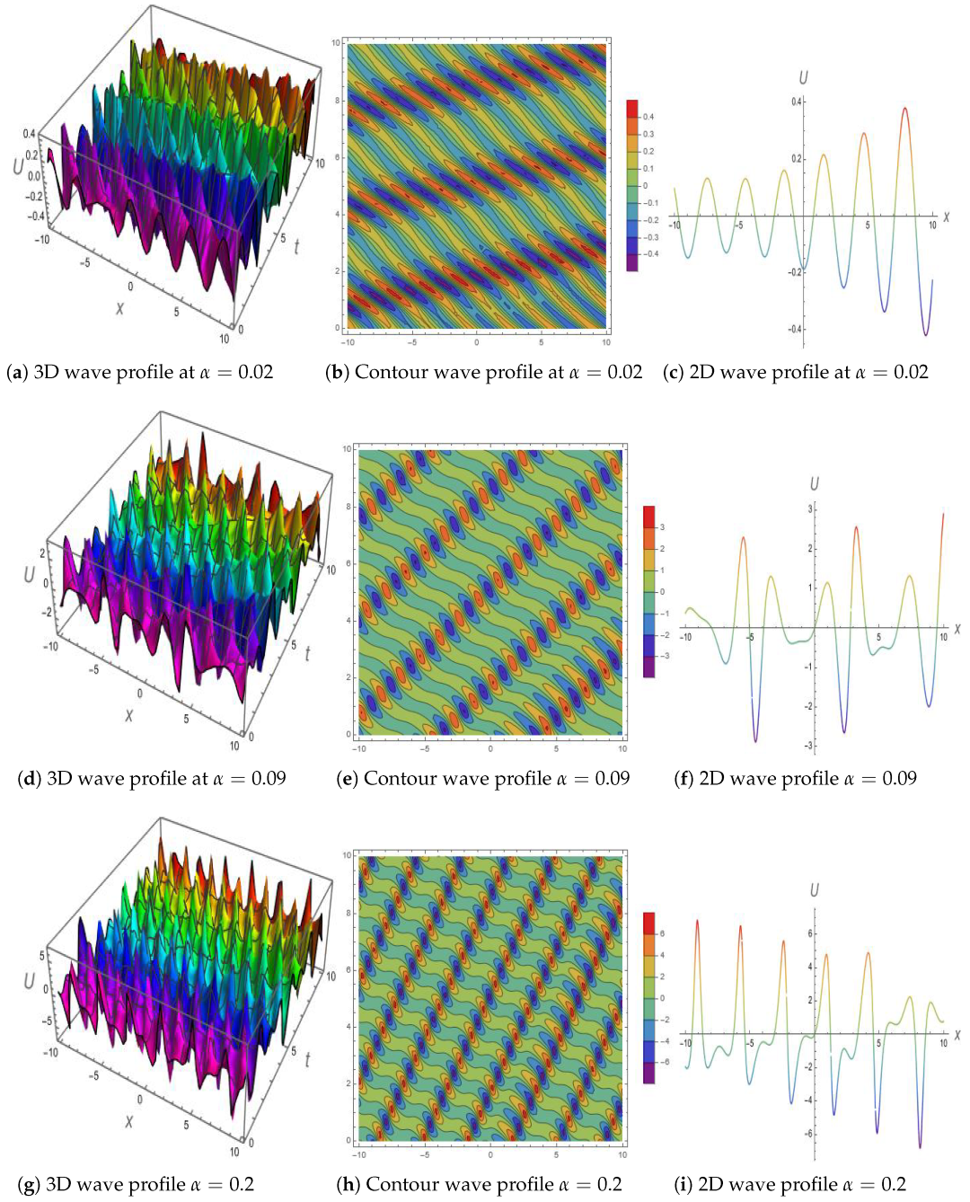
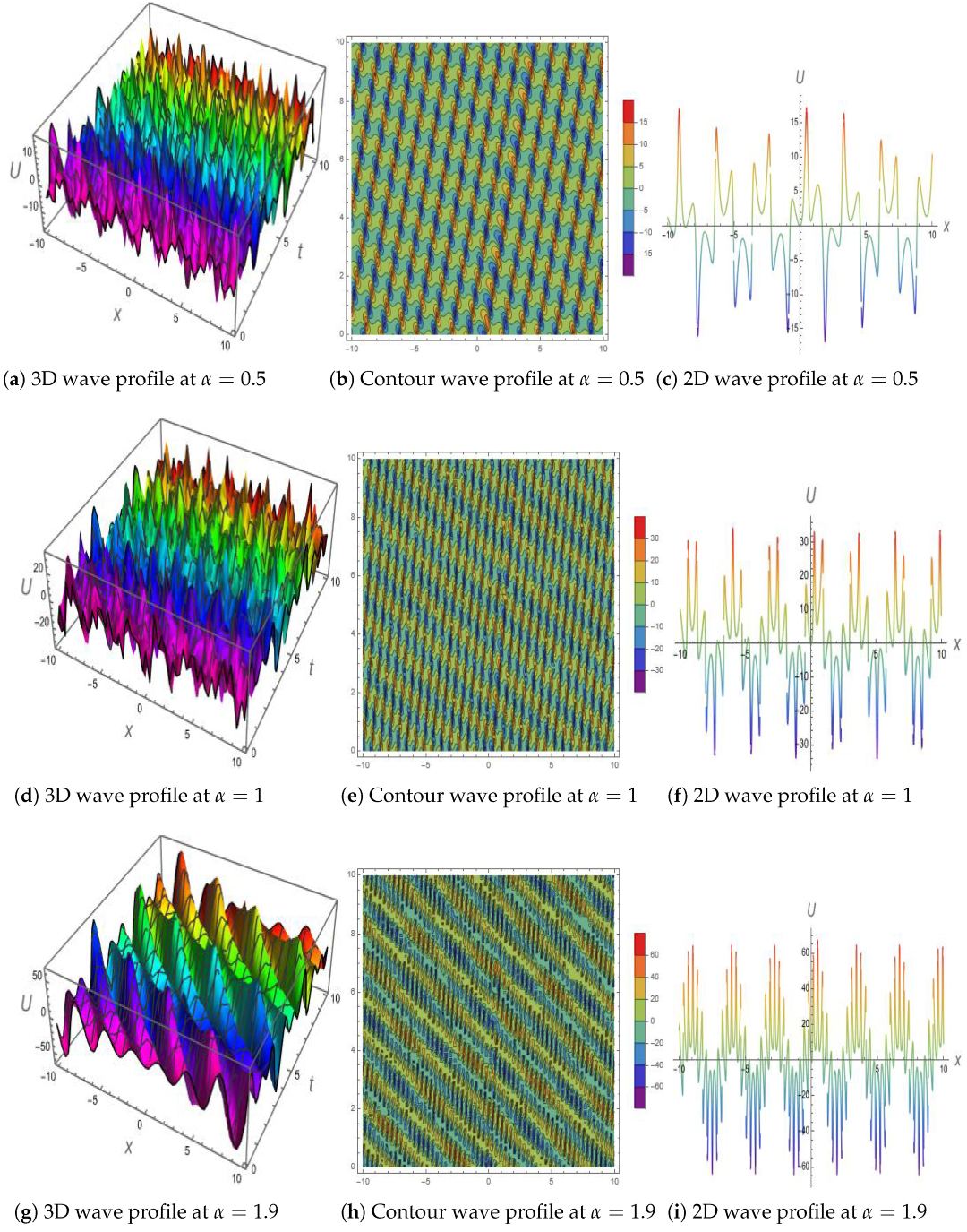
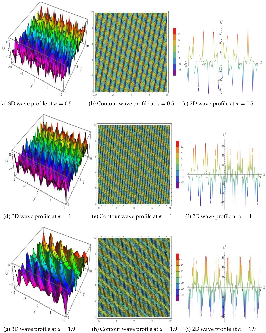
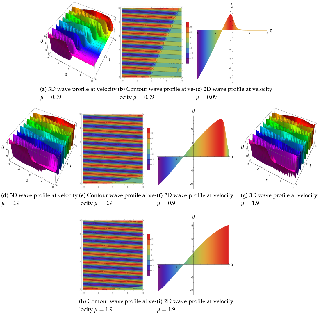
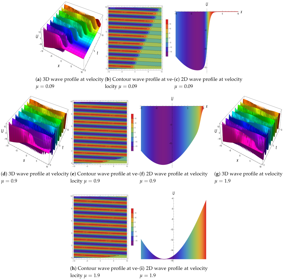
4. Graphical Discussion

In this section, we present a detailed graphical analysis of the model under discussion. The complex solution U 3 ( x , t ) is graphically presented by taking appropriate values of ρ = 5 , m = 7 , n = 2 , a = 5 , b = 0.4 , ϱ = 3 , ζ = 2 , ν = 4 , k 1 = 2 , μ = 0.2 , and λ = 5 . Figure 1 and Figure 2 presented the graphical impact of the wave number on the propagating wave profile for the real part of the solution U 3 ( x , t ) . Figure 3 and Figure 4 presented the graphical impact of the wave number on the propagating wave profile for the imaginary part of the solution U 3 ( x , t ) . Figure 5 and Figure 6 presented the graphical impact of the soliton speed on the propagating wave profile for the real and imaginary parts of the solution in Equation (98) at α = 0.09 , ρ = 5 , a = 0.5 , b = 0.4 , ϱ = 3 , k 1 = 0.1 , and λ = 5 .

5. Conclusions

In this research, we utilized generalized approaches to examine the nonlinear dissipative Schrödinger equation. The established solitonic structures and exact solutions were addressed with a new extended direct algebraic equation technique and Nucci’s reduction, respectively. As a result, we obtained:
  • The mixed complex solitary shock solution, singular solution, mixed shock singular solution, mixed trigonometric solution, mixed singular solution, exact solution, mixed periodic solution, and mixed hyperbolic solution, as well as the periodic solution.
  • The first integral was developed for the nonlinear dissipative Schrödinger equation.
  • A 2D, 3D, and contour visualization was presented, and it was observed that the dissipative parameter and velocity of the soliton were responsible for controlling the amplitude of the propagating wave.
It is hoped that this study will be important for analysts and researchers for improving experimental work, and that it can be expanded in a way that includes multiple solitons, lump interactions, and rogue wave breather types.

Author Contributions

Conceptualization, W.A.F.; Software, M.A.B. and M.A.E.-R.; Formal analysis, S.O. and M.S.; Investigation, W.A.F. and M.S.; Resources, M.A.E.-R.; Writing—original draft, M.A.B.; Writing—review & editing, S.O. and W.A.F.; Supervision, M.S. All authors have read and agreed to the published version of the manuscript.

Funding

The authors acknowledge King Khalid University, Abha, Saudi Arabia, for funding this work through the Large Group Project under grant number RGP 2/73/43.

Institutional Review Board Statement

Not applicable.

Informed Consent Statement

Not applicable.

Data Availability Statement

All of the data are within the manuscript.

Acknowledgments

Magda Abd El-Rahman extends their appreciation to the Deanship of Scientific Research at King Khalid University, Abha, Saudi Arabia.

Conflicts of Interest

The authors declare no conflict of interest.

References

  1. Berezin, F.A.; Shubin, M. The Schrödinger Equation; Springer Science and Business Media: Cham, Switzerland, 2012; Volume 66. [Google Scholar]
  2. Dodson, B. Defocusing Nonlinear Schrödinger Equations; Cambridge University Press: Cambridge, UK, 2019; Volume 217. [Google Scholar]
  3. Malomed, B. Nonlinear Schrödinger Equations. In Encyclopedia of Nonlinear Science; Scott, A., Ed.; Routledge: New York, NY, USA, 2005; pp. 639–643. [Google Scholar]
  4. Seadawy, A.R.; Ali, A.; Albarakati, W.A. Analytical wave solutions of the (2 + 1)-dimensional first integro-differential Kadomtsev-Petviashivili hierarchy equation by using modified mathematical methods. Results Phys. 2019, 15, 102775. [Google Scholar] [CrossRef]
  5. Liu, X.; Zhang, H.; Liu, W. The dynamic characteristics of pure-quartic solitons and soliton molecules. Appl. Math. Model. 2022, 102, 305–312. [Google Scholar] [CrossRef]
  6. Wang, T.Y.; Zhou, Q.; Liu, W.J. Soliton fusion and fission for the high-order coupled nonlinear Schrödinger system in fiber lasers. Chin. Phys. B 2022, 31, 020501. [Google Scholar] [CrossRef]
  7. Ma, G.; Zhao, J.; Zhou, Q.; Biswas, A.; Liu, W. Soliton interaction control through dispersion and nonlinear effects for the fifth-order nonlinear Schrödinger equation. Nonlinear Dyn. 2021, 106, 2479–2484. [Google Scholar] [CrossRef]
  8. Mo, Y.; Ling, L.; Zeng, D. Data-driven vector soliton solutions of coupled nonlinear Schrödinger equation using a deep learning algorithm. Phys. Lett. A 2022, 421, 127739. [Google Scholar] [CrossRef]
  9. Jiang, C.; Cui, J.; Qian, X.; Song, S. High-order linearly implicit structure-preserving exponential integrators for the nonlinear Schrödinger equation. J. Sci. Comput. 2022, 90, 1–27. [Google Scholar] [CrossRef]
  10. Chen, J.; Luan, Z.; Zhou, Q.; Alzahrani, A.K.; Biswas, A.; Liu, W. Periodic soliton interactions for higher-order nonlinear Schrödinger equation in optical fibers. Nonlinear Dyn. 2020, 100, 2817–2821. [Google Scholar] [CrossRef]
  11. Cazenave, T.; Han, Z.; Naumkin, I. Asymptotic behavior for a dissipative nonlinear Schrödinger equation. Nonlinear Anal. 2021, 205, 112243. [Google Scholar] [CrossRef]
  12. López, J.L. A quantum approach to Keller-Segel dynamics via a dissipative nonlinear Schrödinger equation. Discret. Contin. Dyn. Syst. 2021, 41, 2601. [Google Scholar] [CrossRef]
  13. Weng, W.; Zhang, G.; Zhang, M.; Zhou, Z.; Yan, Z. Semi-rational vector rogon–soliton solutions and asymptotic analysis for any n-component nonlinear Schrödinger equation with mixed boundary conditions. Phys. D Nonlinear Phenom. 2022, 432, 133150. [Google Scholar] [CrossRef]
  14. Younas, U.; Seadawy, A.R.; Younis, M.; Rizvi, S.T.R. Optical solitons and closed form solutions to the (3 + 1)-dimensional resonant Schrödinger dynamical wave equation. Int. J. Mod. Phys. B 2020, 34, 2050291. [Google Scholar] [CrossRef]
  15. Rehman, H.U.; Seadawy, A.R.; Younis, M.; Rizvi, S.T.R.; Anwar, I.; Baber, M.Z.; Althobaiti, A. Weakly nonlinear electron-acoustic waves in the fluid ions propagated via a (3 + 1)-dimensional generalized Korteweg–de-Vries–Zakharov–Kuznetsov equation in plasma physics. Results Phys. 2022, 33, 105069. [Google Scholar] [CrossRef]
  16. Akram, G.; Sarfraz, M. Multiple optical soliton solutions for CGL equation with Kerr law nonlinearity via extended modified auxiliary equation mapping method. Optik 2021, 242, 167258. [Google Scholar] [CrossRef]
  17. Akram, G.; Gillani, S.R. Sub pico-second Soliton with Triki–Biswas equation by the extended ( G G 2 )-expansion method and the modified auxiliary equation method. Optik 2021, 229, 166227. [Google Scholar] [CrossRef]
  18. Sadaf, M.; Arshed, S.; Akram, G. Exact soliton and solitary wave solutions to the Fokas system using two variables ( G G , 1 G -expansion technique and generalized projective Riccati equation method. Optik 2022, 268, 169713. [Google Scholar] [CrossRef]
  19. Kumar, S.; Almusawa, H.; Hamid, I.; Akbar, M.A.; Abdou, M.A. Abundant analytical soliton solutions and Evolutionary behaviors of various wave profiles to the Chaffee–Infante equation with gas diffusion in a homogeneous medium. Results Phys. 2021, 30, 104866. [Google Scholar] [CrossRef]
  20. Kumar, S.; Kumar, A. Abundant closed-form wave solutions and dynamical structures of soliton solutions to the (3 + 1)-dimensional BLMP equation in mathematical physics. J. Ocean. Eng. Sci. 2022, 7, 178–187. [Google Scholar] [CrossRef]
  21. Kumar, S.; Almusawa, H.; Kumar, A. Some more closed-form invariant solutions and dynamical behavior of multiple solitons for the (2+ 1)-dimensional rdDym equation using the Lie symmetry approach. Results Phys. 2021, 24, 104201. [Google Scholar] [CrossRef]
  22. Jhangeer, A.; Faridi, W.A.; Asjad, M.I.; Akgül, A. Analytical study of soliton solutions for an improved perturbed Schrödinger equation with Kerr law non-linearity in non-linear optics by an expansion algorithm. Partial. Differ. Equations Appl. Math. 2021, 4, 100102. [Google Scholar] [CrossRef]
  23. Faridi, W.A.; Asjad, M.I.; Eldin, S.M. Exact Fractional Solution by Nucci’s Reduction Approach and New Analytical Propagating Optical Soliton Structures in Fiber-Optics. Fractal Fract. 2022, 6, 654. [Google Scholar] [CrossRef]
  24. Asjad, M.I.; Faridi, W.A.; Jhangeer, A.; Abu-Zinadah, H.; Ahmad, H. The fractional comparative study of the non-linear directional couplers in non-linear optics. Results Phys. 2021, 27, 104459. [Google Scholar] [CrossRef]
  25. Faridi, W.A.; Asjad, M.I.; Jhangeer, A. The fractional analysis of fusion and fission process in plasma physics. Phys. Scr. 2021, 96, 104008. [Google Scholar] [CrossRef]
  26. Ma, G.; Zhou, Q.; Yu, W.; Biswas, A.; Liu, W. Stable transmission characteristics of double-hump solitons for the coupled Manakov equations in fiber lasers. Nonlinear Dyn. 2021, 106, 2509–2514. [Google Scholar] [CrossRef]
  27. Inan, I.E.; Inc, M.; Rezazadeh, H.; Akinyemi, L. Optical solitons of (3+ 1) dimensional and coupled nonlinear Schrodinger equations. Opt. Quantum Electron. 2022, 54, 1–15. [Google Scholar] [CrossRef]
  28. Kudryashov, N.A. Almost general solution of the reduced higher-order nonlinear Schrödinger equation. Optik 2021, 230, 166347. [Google Scholar] [CrossRef]
  29. Kudryashov, N.A. Optical solitons of the resonant nonlinear Schrödinger equation with arbitrary index. Optik 2021, 235, 166626. [Google Scholar] [CrossRef]
  30. Wang, K.J.; Wang, G.D. Variational theory and new abundant solutions to the (1+ 2)-dimensional chiral nonlinear Schrödinger equation in optics. Phys. Lett. A 2021, 412, 127588. [Google Scholar] [CrossRef]
  31. Faridi, W.A.; Asjad, M.I.; Jarad, F. The fractional wave propagation, dynamical investigation, and sensitive visualization of the continuum isotropic bi-quadratic Heisenberg spin chain process. Results Phys. 2022, 43, 106039. [Google Scholar] [CrossRef]
  32. Faridi, W.A.; Asjad, M.I.; Toseef, M.; Amjad, T. Analysis of propagating wave structures of the cold bosonic atoms in a zig-zag optical lattice via comparison with two different analytical techniques. Opt. Quantum Electron. 2022, 54, 1–24. [Google Scholar] [CrossRef] [PubMed]
  33. Farman, M.; Akgül, A.; Tekin, M.T.; Akram, M.M.; Ahmad, A.; Mahmoud, E.E.; Yahia, I.S. Fractal fractional-order derivative for HIV/AIDS model with Mittag-Leffler kernel. Alex. Eng. J. 2022, 61, 10965–10980. [Google Scholar] [CrossRef]
  34. Modanli, M.; Göktepe, E.; Akgül, A.; Alsallami, S.A.; Khalil, E.M. Two approximation methods for fractional order Pseudo-Parabolic differential equations. Alex. Eng. J. 2022, 61, 10333–10339. [Google Scholar] [CrossRef]
  35. Partohaghighi, M.; Mirtalebi, Z.; Akgül, A.; Riaz, M.B. Fractal–fractional Klein–Gordon equation: A numerical study. Results Phys. 2022, 42, 105970. [Google Scholar] [CrossRef]
  36. Iqbal, M.S.; Yasin, M.W.; Ahmed, N.; Akgül, A.; Rafiq, M.; Raza, A. Numerical simulations of nonlinear stochastic Newell-Whitehead-Segel equation and its measurable properties. J. Comput. Appl. Math. 2023, 418, 114618. [Google Scholar] [CrossRef]
  37. Bekir, A.; Younis, M.; Rizvi, S.T.; Sardar, A.; Mahmood, S.A. On traveling wave solutions: The decoupled nonlinear Schrödinger equations with inter modal dispersion. Comput. Methods Differ. Equations 2021, 9, 52–62. [Google Scholar]
  38. Younis, M.; Ali, S.; Rizvi, S.T.R.; Tantawy, M.; Tariq, K.U.; Bekir, A. Investigation of solitons and mixed lump wave solutions with (3 + 1)-dimensional potential-YTSF equation. Commun. Nonlinear Sci. Numer. Simul. 2021, 94, 105544. [Google Scholar] [CrossRef]
  39. Rizvi, S.T.R.; Bibi, I.; Younis, M.; Bekir, A. Interaction properties of solitons for a couple of nonlinear evolution equations. Chin. Phys. B 2021, 30, 010502. [Google Scholar] [CrossRef]
  40. Attia, N.; Akgül, A. A reproducing kernel Hilbert space method for nonlinear partial differential equations: Applications to physical equations. Phys. Scr. 2022, 97, 104001. [Google Scholar] [CrossRef]
  41. Chen, S.; Baronio, F.; Soto-Crespo, J.M.; Liu, Y.; Grelu, P. Chirped Peregrine solitons in a class of cubic-quintic nonlinear Schrödinger equations. Phys. Rev. E 2016, 93, 062202. [Google Scholar] [CrossRef] [Green Version]
  42. Baronio, F.; Chen, S.; Trillo, S. Resonant radiation from Peregrine solitons. Opt. Lett. 2020, 45, 427–430. [Google Scholar] [CrossRef]
  43. Seadawy, A.R.; Rizvi, S.T.; Ahmed, S.; Ahmad, A. Study of dissipative NLSE for dark and bright, multiwave, breather and M-shaped solitons along with some interactions in monochromatic waves. Opt. Quantum Electron. 2022, 54, 1–20. [Google Scholar] [CrossRef]
Figure 1. 3D, Contour and 2D impact of wave number α on the Real part of solution U 3 .
Fractalfract 07 00038 g001
Figure 2. The influence of different wave numbers α on the Real part of solution U 3 .
Fractalfract 07 00038 g002
Figure 3. 3D, Contour and 2D impact of wave number α on the Imaginary part of solution U 3 .
Fractalfract 07 00038 g003
Figure 4. The effect of different wave numbers α on the Imaginary part of solution U 3 .
Fractalfract 07 00038 g004
Figure 5. For the real part of solution Equation (98), the impact of velocity is seen in 3D, 2D, and contour.
Fractalfract 07 00038 g005
Figure 6. For the Imaginary part of solution Equation (98), the impact of velocity is seen in 3D, 2D, and contour graphs.
Fractalfract 07 00038 g006
Disclaimer/Publisher’s Note: The statements, opinions and data contained in all publications are solely those of the individual author(s) and contributor(s) and not of MDPI and/or the editor(s). MDPI and/or the editor(s) disclaim responsibility for any injury to people or property resulting from any ideas, methods, instructions or products referred to in the content.

