Analytical and Computational Problems Related to Fractional Gaussian Noise

Abstract

We study the projection of an element of fractional Gaussian noise onto its neighbouring elements. We prove some analytic results for the coefficients of this projection. In particular, we obtain recurrence relations for them. We also make several conjectures concerning the behaviour of these coefficients, provide numerical evidence supporting these conjectures, and study them theoretically in particular cases. As an auxiliary result of independent interest, we investigate the covariance function of fractional Gaussian noise, prove that it is completely monotone for $H>1/2$, and, in particular, monotone, convex, log-convex along with further useful properties.

1. Introduction

This paper is about some (conjectured) properties of the projection of an element of fractional Gaussian noise onto the neighbouring elements. Unfortunately, not all our conjectures are amenable to analytical proofs, while numerical experiments confirm their validity. This is indeed rather strange, as the properties of fractional Brownian motion and its increments have been thoroughly studied, attracting a lot of research efforts resulting in countless papers and several books, e.g., [1,2,3,4]. These books are mostly devoted to the stochastic analysis of fractional processes, the properties of their trajectories, distributional properties of certain functionals of the paths, and related issues. Note that such interest and the large number of theoretical studies related to Gaussian fractional noises is due to the wide range of applications of such processes and its properties: existence of memory combined with self-similarity and stationarity. In particular, fractional Gaussian noises appear in the investigation of the behaviour of anomalous diffusion and solutions of fractional diffusion equations, including numerical schemes [5,6,7], information capacity of a non-linear neuron model [8], statistical inference [9,10], entropy calculation [11,12], extraction of the quantitative information from recurrence plots [13] and many others. There is, however, an area where much less is known: problems relating to the covariance matrix of fractional Brownian motion and fractional Gaussian noise in high dimensions, and its determinant. Computational features of the covariance matrices are widely used for simulations and in various applications, see, for example, [14,15,16,17]. The problem considered in the present paper arose in the following way: In [18], the authors construct a discrete process that converges weakly to a fractional Brownian motion (fBm) $B^H=\{B_t^H,t\ge 0\}$ with Hurst parameter $H\in (\frac{1}{2},1)$. The construction of this process is based on the Cholesky decomposition of the covariance matrix of the fractional Gaussian noise (fGn). Several interesting properties of this decomposition are proved in [18], such as the positivity of all elements of the corresponding triangular matrix and the monotonicity along its main diagonal. Numerical examples suggest also the conjecture, that one has monotonicity along all diagonals of this matrix. However, the analytic proof of this fact remains an open problem. Studying this problem, the authors of [18] establish a connection between the predictor’s coefficients—that is, the coefficients of the projection of any value of a stationary Gaussian process onto finitely many subsequent elements—and the Cholesky decomposition of the covariance matrix of the process. It turns out that the positivity of the coefficients of the predictor implies the monotonicity along the diagonals of the triangular matrix of the Cholesky decomposition of fGn, which is sufficient for the monotonicity along the columns of the triangular matrix in the Cholesky decomposition of fBm itself; this property, in turn, ensures the convergence of a wide class of discrete-time schemes to a fractional Brownian motion. We will see in Section 2.1 below that the coefficients of the predictor can be found as the solution to a system of linear equations, whose coefficient matrix coincides with the covariance matrix of fGn. This enables us to reduce the monotonicity problem for the Cholesky decomposition to proving the positivity of the solution to a linear system of equations. However, see Section 2, even in the particular case of a $3\times 3$-matrix, an analytic proof of positivity of all coefficients is a non-trivial problem. For the moment, we have only a partial solution. Therefore, we formulate the following conjecture:

Conjecture 1.

If $H>1/2$, then the coefficients of the projection of any element of fractional Gaussian noise onto any finite number of its subsequent elements are strictly positive.

We shall discuss this conjecture in Section 2 in more detail. Due to stationarity, it is sufficient to establish Conjecture 1 for the projection of ${\Delta }_1$ onto ${\Delta }_2,\dots ,{\Delta }_n$, i.e., for the conditional expectation

$$\begin{array}{c}\mathbb{E}\left({\Delta }_1\mid {\Delta }_2,\dots ,{\Delta }_n\right),n\ge 3,\end{array}$$

where $B^H$ denotes fBM and ${\Delta }_k=B_k^H-B_{k-1}^H$. Having computational evidence but lacking an analytical proof for Conjecture 1, we provide in this paper a wide range of associated properties of coefficients, some with an analytic proof, and some obtained using various computational tools. It is, in particular, interesting to study the asymptotic behaviour of the coefficients as $H\uparrow 1$. This is particularly interesting since $H=1$ fractional Brownian motion $B^1$ is degenerate, i.e., $B_t^1=t\xi$, where $\xi$∼$\mathcal{N}(0,1)$, and $\mathcal{N}(0,1)$ denotes the standard normal distribution. Consequently, ${\Delta }_k$∼$\mathcal{N}(0,1)$ for all $k\ge 1$, and

$$\begin{array}{c}\mathbb{E}\left({\Delta }_1\mid {\Delta }_2,\dots ,{\Delta }_n\right)=\sum _{k=2}^n{\alpha }_k{\Delta }_k\sim \mathcal{N}(0,1)\end{array}$$

for any convex combination, ${\alpha }_k\ge 0,{\sum }_{k=2}^n{\alpha }_k=1$. This shows that in the case $H=1$, the values of the coefficients are indefinite, and therefore they cannot define the asymptotic behaviour of the prelimit coefficients as $H\uparrow 1$. It will be very “elegant” if all coefficients tend to ${(n-1)}^{-1}$; however, in reality their asymptotic behaviour is different, see Section 2.3. Another interesting question are the relations between the coefficients. It is natural to assume that they decrease as k increases, but the situation here is also more involved, essentially depending on the value of H. In Section 2.4, we prove some recurrence relations between the coefficients. These relations lead to a computational algorithm which is more efficient than solving the system of equations as described in Section 2.1. Finally, it turns out that the positivity of the first coefficient can be proven analytically for all values of n; this result is established in Section 2.5.

We close the paper with a few numerical examples, supporting our theoretical results and conjectures. In particular, we compute the coefficients for all $n\le 10$ and for various values of H, and discuss their behaviour. Additionally, we compare different calculation methods for the coefficients in terms of computing time, and we demonstrate the advantage of the approach via the recurrence of formulae in most cases.

The paper is organized as follows: Section 2 contains almost all properties of the predictor’s coefficients that can be established analytically, and it introduces the system of linear equations for these coefficients and some properties of the coefficients of this system. We consider in detail two particular cases: $n=3$ and $n=4$. In these cases, we prove the positivity of all coefficients, establish some relations between them, and study the asymptotic behaviour as $H\uparrow 1$. We also obtain recurrence relations for the coefficients, and prove that for all values of n, the first coefficient is positive. Section 3 contains some numerical illustrations of the properties and conjectures from Section 1 and Section 2. In Section 3.3, we briefly discuss some observations concerning the case $H<1/2$.

2. Analytical Properties of the Coefficients

Let $B^H=\left\{B_t^H,t\ge 0\right\}$ be a fractional Brownian motion (fBm) with Hurst index $H\in (\frac{1}{2},1)$, that is, a centered Gaussian process with covariance function of the form

$$\mathbb{E}{B}_t^H{B}_s^H=\frac{1}{2}\left(t^{2H}+s^{2H}-{\left|t-s\right|}^{2H}\right).$$

(1)

We use

$${\Delta }_n=B_n^H-B_{n-1}^H,n=1,2,3,\dots .$$

for the nth increment of fBM. It is well known that the process $B^H$ has stationary increments, which implies that $\left\{{\Delta }_n,n\ge 1\right\}$ is a stationary Gaussian sequence (known as fractional Gaussian noise—fGn for short). It follows from (1) that its autocovariance function is given by

$$\begin{array}{c}{\rho }_k=\mathbb{E}{\Delta }_1{\Delta }_{k+1}=\frac{1}{2}\left({\left|k+1\right|}^{2H}-{2\left|k\right|}^{2H}+{\left|k-1\right|}^{2H}\right),k\ge 1.\end{array}$$

(2)

Obviously, ${\rho }_0=1$.

Now, let us consider the projection of ${\Delta }_1$ onto ${\Delta }_2,\dots ,{\Delta }_n$, i.e., the conditional expectation $\mathbb{E}\left({\Delta }_1\mid {\Delta }_2,\dots ,{\Delta }_n\right)$. Since the joint distribution of $({\Delta }_1,\dots ,{\Delta }_n)$ is centered and Gaussian, we obtain the following relation from the theorem on normal correlation (see, for example, Theorem 3.1 in [19]):

$$\begin{array}{c}\mathbb{E}\left({\Delta }_1\mid {\Delta }_2,\dots ,{\Delta }_n\right)=\sum _{k=2}^n{\Gamma }_n^k{\Delta }_k,n\ge 2,\end{array}$$

(3)

where ${\Gamma }_n^k\in \mathbb{R}$. Our Conjecture 1 means that all the coefficients ${\Gamma }_n^k$ for $n=2,3\dots$, $k=2,3,\dots ,n$, are strictly positive (We have formulated it in more general form, i.e., for any element ${\Delta }_j$, because, by stationarity, the projection $\mathbb{E}\left({\Delta }_j\mid {\Delta }_{j+1},\dots ,{\Delta }_{j+n-1}\right)$ for any j has the same distribution as $\mathbb{E}\left({\Delta }_1\mid {\Delta }_2,\dots ,{\Delta }_n\right)$).

Let us consider two approaches to the calculation of the coefficients ${\Gamma }_n^k$. The first method is straightforward; it involves solving of the system of linear equations. The second one is based on recurrence relations for the ${\Gamma }_n^k$.

2.1. System of Linear Equations for Coefficients

Multiplying both sides of (3) by ${\Delta }_l$, $2\le l\le n$ and taking expectations yields

$$\begin{array}{c}\mathbb{E}{\Delta }_1{\Delta }_l=\sum _{k=2}^n{\Gamma }_n^k\mathbb{E}{\Delta }_k{\Delta }_l,2\le l\le n.\end{array}$$

Due to stationarity,

$$\begin{array}{c}\mathbb{E}{\Delta }_k{\Delta }_l={\rho }_{|l-k|}.\end{array}$$

This leads to the following system of linear equations for the coefficients ${\Gamma }_n^k$, $k=2,\dots ,n$:

$$\begin{array}{c}{\rho }_{l-1}=\sum _{k=2}^n{\Gamma }_n^k{\rho }_{|l-k|},2\le l\le n.\end{array}$$

(4)

We can solve this using Cramer’s rule,

$$\begin{array}{c}{\Gamma }_n^k=\frac{det{A}_k}{detA},\end{array}$$

where

$$\begin{array}{cc}\hfill A& =\left(\begin{array}{ccccccc}1& {\rho }_1& {\rho }_2& \cdots & {\rho }_k& \cdots & {\rho }_{n-2}\\ {\rho }_1& 1& {\rho }_1& \cdots & {\rho }_{k-1}& \cdots & {\rho }_{n-3}\\ ⋮& ⋮& ⋮& & ⋮& & ⋮\\ {\rho }_{n-2}& {\rho }_{n-3}& {\rho }_{n-4}& \cdots & {\rho }_{n-k-1}& \cdots & 1\end{array}\right)\hfill \end{array}$$

(5)

and $A_k$ is the matrix A with its kth column vector replaced by ${({\rho }_1,\dots ,{\rho }_{n-1})}^{\top }$:

$$\begin{array}{cc}\hfill A_k& =\left(\begin{array}{ccccccc}1& {\rho }_1& {\rho }_2& \cdots & \stackrel{\stackrel{k\mathrm{th} \mathrm{column}}{⎴}}{{\rho }_1}& \cdots & {\rho }_{n-2}\\ {\rho }_1& 1& {\rho }_1& \cdots & {\rho }_2& \cdots & {\rho }_{n-3}\\ ⋮& ⋮& ⋮& & ⋮& & ⋮\\ {\rho }_{n-2}& {\rho }_{n-3}& {\rho }_{n-4}& \cdots & {\rho }_{n-1}& \cdots & 1\end{array}\right).\hfill \end{array}$$

(6)

Remark 1.

It is known that the finite-dimensional distributions of $B^H$ have a nonsingular covariance matrix; in particular, for any $0<t_1<\cdots <t_n$, the values $B_{t_1}^H,\dots ,B_{t_n}^H$ are linearly independent; see Theorem 1.1 in [20] and its proof. Obviously, a similar statement holds for fractional Gaussian noise, since the vector $({\Delta }_1,\dots ,{\Delta }_n)$ is a nonsingular linear transform of $(B_1^H,\dots ,B_n^H)$. In other words, $detA\ne 0$; moreover, if ${\sum }_k{\alpha }_k{\Delta }_k=0$ a.s., then ${\alpha }_k=0$ for all k.

2.2. Relations between the Values ${\rho }_k$

In order to establish analytic properties of the coefficients ${\Gamma }_n^k$, we need several auxiliary results on the properties of the sequence $\left\{{\rho }_k,k\in {\mathbb{Z}}_{+}\right\}$. We start with a useful relation between ${\rho }_1$, ${\rho }_2$ and ${\rho }_3$.

Lemma 1.

The following equality holds:

$$\begin{array}{c}{\rho }_2-{\rho }_1^2=\frac{1}{2}({\rho }_1-{\rho }_3).\end{array}$$

(7)

Proof. 

Using the self-similarity of fBm and the stationarity of its increments, we obtain

$$\begin{array}{cc}\hfill 2^{2H}{\rho }_1& =2^{2H}\mathbb{E}{B}_1^H(B_2^H-B_1^H)\hfill \\ \hfill & =\mathbb{E}{B}_2^H(B_4^H-B_2^H)\hfill \\ \hfill & =\mathbb{E}(B_2^H-B_1^H)(B_4^H-B_2^H)+\mathbb{E}{B}_1^H(B_4^H-B_2^H)\hfill \\ \hfill & =\mathbb{E}{\Delta }_2({\Delta }_3+{\Delta }_4)+\mathbb{E}{\Delta }_1({\Delta }_3+{\Delta }_4)\hfill \\ \hfill & ={\rho }_1+2{\rho }_2+{\rho }_3.\hfill \end{array}$$

Note that by (2), ${\rho }_1=2^{2H-1}-1$, whence $2^{2H}=2{\rho }_1+2$. Thus, we arrive at

$$\begin{array}{c}(2{\rho }_1+2){\rho }_1={\rho }_1+2{\rho }_2+{\rho }_3.\end{array}$$

which is equivalent to (7).    □

Remark 2.

The inequality ${\rho }_1^2<{\rho }_2$ was proved in [18] (p. 28) by analytic methods. In this paper, we improve this result in two directions: we obtain an explicit expression for ${\rho }_2-{\rho }_1^2$ and we prove the sharper bound ${\rho }_1^2<{\rho }_3$; see Lemma 3 below.

Many important properties of the covariance function of a fractional Gaussian noise (such as monotonicity, convexity and log-convexity) follow from the more general property of complete monotonicity, which is stated in the next lemma. To formulate it, let us introduce the function

$$\begin{array}{c}\rho \left(x\right)=\rho (H,x)=\frac{1}{2}\left({|x+1|}^{2H}-{2\left|x\right|}^{2H}+{|x-1|}^{2H}\right),x\ge 0.\end{array}$$

Lemma 2.

1.

The function $\rho :(0,\infty )\to \mathbb{R}$ is convex if $H>1/2$ and concave if $H<1/2$.

2.

If $H>1/2$, then the function ρ is completely monotone(CM)on $(1,\infty )$, that is, $\rho \in C^{\infty }(1,\infty )$ and

$$\begin{array}{c}{(-1)}^n{\rho }^{\left(n\right)}\left(x\right)\ge 0\mathrm{for}\mathrm{all}n\in \mathbb{N}\cup \left\{0\right\}\mathrm{and}x>1.\end{array}$$

(8)

3.

If $H<1/2$, then the function $-\rho$ is completely monotone on $(1,\infty )$.

Proof. 

1. Using the elementary relation $\frac{d}{dx}{\left|x\right|}^{2H}=2H\mathrm{sgn}\left(x\right){\left|x\right|}^{2H-1}$, it is not hard to see that

$$\begin{array}{cc}\hfill \rho \left(x\right)& =\frac{1}{2}\left({|x+1|}^{2H}-{\left|x\right|}^{2H}\right)-\frac{1}{2}\left({\left|x\right|}^{2H}-{|x-1|}^{2H}\right)\hfill \\ \hfill & =H(2H-1){\int }_0^1{\int }_{-t}^t{|x+s|}^{2H-2}dsdt.\hfill \end{array}$$

(9)

Since $x\mapsto {|x+s|}^{2H-2}$ is convex, and since convex functions are a convex cone which is closed under pointwise convergence, the double integral appearing in the representation of $\rho \left(x\right)$ is again convex. Thus, $\rho \left(x\right)$ is convex or concave according to $2H-1>0$ or $2H-1<0$, respectively.

2. Let $H>\frac{1}{2}$ and $x\ge 1$. Then, Formula (9) remains valid if we replace $|x+s|$ with $(x+s)$. But ${(x+s)}^{2H-2}$ is CM and so $\rho \left(x\right)$ is an integral mixture of CM-functions. Since CM is a convex cone which is closed under pointwise convergence, cf. Corollary 1.6 in [21], we see that $\rho$ is CM on $(1,\infty )$.

3. The above arguments holds true in the case $H<\frac{1}{2}$; the only difference is that in this case, the factor $(2H-1)$ is negative.    □

Remark 3.

1. Since $x\mapsto \rho (x+1)$ is a CM function on $(0.\infty )$, it admits the representation $\rho (x+1)=a+{\int }_0^{\infty }{e}^{-xt}\mu \left(dt\right)$, for some positive measure μ on $[0,\infty )$ and $a\ge 0$, see, for example, Theory 1.4 in [21]. Taking into account that $\rho (+\infty )=0$, it is not hard to see that $a=0$, i.e.,

$$\begin{array}{c}\rho (x+1)={\int }_0^{\infty }{e}^{-xt}\mu \left(dt\right).\end{array}$$

(10)

2. The function ρ can be represented in the form $\rho (x+1)={\Delta }_1^2{f}_H\left(x\right)$, where we write ${\Delta }_{1}f\left(x\right):=$$f(x+1)-f\left(x\right)$ for the step-1 difference operator, and $f_H\left(x\right):=\frac{1}{2}{x}^{2H}$. Then the second statement of Lemma 2 follows from the more general result: if f is CM on $(0,\infty )$, then ${\Delta }_2^{1}f$ is CM. Indeed, since CM is a closed convex cone, it is enough to verify the claim for the “basic” CM function $f\left(x\right)=e^{-tx}$, where $t\ge 0$ is a parameter. Now we have

$$\begin{array}{c}{\Delta }_1^{2}f\left(x\right)=e^{-(x+2)t}-2e^{-(x+1)t}+e^{-xt}=e^{-xt}{(e^{-t}-1)}^2,\end{array}$$

and this is clearly a completely monotone function.

3. The argument which we used in the proof of Lemma 2. proves a bit more: The function $x\mapsto \rho (H,x)$ is for $x\ge 1$ and $H>1/2$ even a Stieltjes function, i.e., a double Laplace transform. To see this, we note that the kernel $x\mapsto {(x+s)}^{2H-2}$ is a Stieltjes function. Further details on Stieltjes functions can be found in [21].

As for the following properties, fractional Brownian with Hurst index $H=1$ is degenerate, i.e., $B_t^1=t\xi$, where $\xi$∼$\mathcal{N}(0,1)$; consequently all ${\rho }_k=1$ and the next set of inequalities are equalities. Therefore, we consider only $1/2<H<1$.

Corollary 1.

Let $H\in (\frac{1}{2},1)$. The sequence $\{{\rho }_k,k\ge 0\}$ has the following properties

1.

Monotonicity and positivity: for any $k\in \mathbb{N}$

$$\begin{array}{c}{\rho }_{k-1}>{\rho }_k>0.\end{array}$$

(11)

2.

Convexity: for any $k\in \mathbb{N}$

$$\begin{array}{c}{\rho }_{k-1}-{\rho }_k>{\rho }_k-{\rho }_{k+1}.\end{array}$$

(12)

3.

Log-convexity: for any $k\in \mathbb{N}$

$$\begin{array}{c}{\rho }_{k-1}{\rho }_{k+1}>{\rho }_k^2.\end{array}$$

(13)

Proof. 

By Lemma 2, the function $\rho \left(x\right)$ is convex on $(0,\infty )$ and completely monotone on $(1,\infty )$; by continuity, we can include the endpoints of each interval.

We begin with the observation that a completely monotone function is automatically log-convex. We show this for $\rho$ using the representation (10): for any $x\ge 0$,

$$\begin{array}{c}\rho (x+1)={\int }_0^{\infty }{e}^{-xt}\mu \left(dt\right),{\rho }^{\prime }(x+1)=-{\int }_0^{\infty }{e}^{-xt}t\mu \left(dt\right),\\ {\rho }^{\prime \prime }(x+1)={\int }_0^{\infty }{e}^{-xt}{t}^2\mu \left(dt\right).\end{array}$$

Thus, the Cauchy–Schwarz inequality yields

$$\begin{array}{c}{\left({\rho }^{\prime }\left(x\right)\right)}^2\le \rho \left(x\right)·{\rho }^{″}\left(x\right)\end{array}$$

(14)

which guarantees that $x\mapsto log\rho (x+1)$ is convex.

Therefore all properties claimed in the statement hold for $k\ge 2$, convexity even for $k\ge 1$, and we only have to deal with the case $k=1$.

Monotonicity for $k=1$: We have to show ${\rho }_0>{\rho }_1$. This follows by direct verification since by (2),

$$\begin{array}{c}{\rho }_0=1\mathrm{and}{\rho }_1=2^{2H-1}-1\end{array}$$

(15)

(recall that $1/2<H<1$).

Log-convexity for $k=1$: In this case, the inequality (13) has the form ${\rho }_2>{\rho }_1^2$. It immediately follows from the representation (7) combined with the monotonicity property (11).    □

The previous lemma implies that ${\rho }_1^2<{\rho }_2$. The following result gives a sharper bound.

Lemma 3.

If $H\in (\frac{1}{2},1)$, then

$$\begin{array}{c}{\rho }_1^2<{\rho }_3.\end{array}$$

(16)

Proof. 

Applying (7), we may write

$$\begin{array}{c}{\rho }_3-{\rho }_1^2={\rho }_3-{\rho }_2+\frac{1}{2}({\rho }_1-{\rho }_3)=\frac{1}{2}({\rho }_1-2{\rho }_2+{\rho }_3)>0,\end{array}$$

because of Statement 2 of Corollary 1.    □

2.3. Particular Cases

We will now consider in detail two particular cases: $n=3$ and $n=4$. In these cases, we prove the positivity of all coefficients ${\Gamma }_n^k$, establish some relations between them, and study the asymptotic behavior as $H\uparrow 1$. In the case $n=3$ everything is established analytically, while in the case $n=4$, the sign of the second coefficient ${\Gamma }_n^3$ and the relation between the second and the third coefficients, ${\Gamma }_n^3$ and ${\Gamma }_n^4$, are verified numerically.

2.3.1. Case $n=3$

In the case $n=3$, the system (4) becomes

$$\begin{array}{c}\left\{\begin{array}{cc}\hfill {\Gamma }_3^2+{\Gamma }_3^3{\rho }_1& ={\rho }_1,\hfill \\ \hfill {\Gamma }_3^2{\rho }_1+{\Gamma }_3^3& ={\rho }_2,\hfill \end{array}\right.\end{array}$$

(17)

whence

$$\begin{array}{c}{\Gamma }_3^2=\frac{{\rho }_1(1-{\rho }_2)}{1-{\rho }_1^2},{\Gamma }_3^3=\frac{{\rho }_2-{\rho }_1^2}{1-{\rho }_1^2}.\end{array}$$

Proposition 1.

For any $H\in (\frac{1}{2},1)$,

$$\begin{array}{c}{\Gamma }_3^2>{\Gamma }_3^3>0.\end{array}$$

Proof. 

Recall that, by Corollary 1 (Statement 1), $1>{\rho }_1>{\rho }_2>\cdots$ Hence, the first inequality ${\Gamma }_3^2>{\Gamma }_3^3$ is equivalent to

$$\begin{array}{c}{\rho }_1(1-{\rho }_2)>{\rho }_2-{\rho }_1^2\mathrm{or}(1+{\rho }_1)({\rho }_1-{\rho }_2)>0,\end{array}$$

which is true due to Corollary 1.

To prove the second inequality ${\Gamma }_3^3>0$, we need to show that ${\rho }_2>{\rho }_1^2$, which was established in Corollary 1.    □

Remark 4.

It is worth pointing out that the positivity (and positive definiteness) of the coefficient matrix together with the positivity of the right-hand side of the system does not imply the positivity of the solution. Indeed, consider the following system with the same coefficients as in (17), but another positive right-hand side, say $(b_1,b_2)$:

$$\begin{array}{c}\left(\begin{array}{cc}1& {\rho }_1\\ {\rho }_1& 1\end{array}\right)\left(\begin{array}{c}{x}_1\\ x_2\end{array}\right)=\left(\begin{array}{c}{b}_1\\ b_2\end{array}\right).\end{array}$$

The solution has the form

$$\begin{array}{c}{x}_1=\frac{b_1-b_2{\rho }_1}{1-{\rho }_1^2},x_2=\frac{b_2-b_1{\rho }_1}{1-{\rho }_1^2}.\end{array}$$

If, for example, $b_2<b_1{\rho }_1$, then $x_1>0$ and $x_2<0$. For the system (17), this condition is written as ${\rho }_2<{\rho }_1^2$, contradicting Corollary 1.

Proposition 2.

$$\begin{array}{cc}\hfill \underset{H\uparrow 1}{lim}{\Gamma }_3^2& =\frac{9log9-8log4}{8log4}\approx 0.783083,\hfill \\ \hfill \underset{H\uparrow 1}{lim}{\Gamma }_3^3& =\frac{8log16-9log9}{8log4}\approx 0.216917.\hfill \end{array}$$

Proof. 

If we take the limit $H\uparrow 1$ in the relations

$$\begin{array}{c}{\rho }_1=2^{2H-1}-1,{\rho }_2=\frac{1}{2}\left(3^{2H}-2^{2H+1}+1\right),\end{array}$$

(18)

we obtain

$$\begin{array}{c}{\rho }_1\to 1,{\rho }_2\to 1,\mathrm{as}H\uparrow 1.\end{array}$$

Therefore,

$$\begin{array}{cc}\hfill \underset{H\uparrow 1}{lim}{\Gamma }_3^2& =\underset{H\uparrow 1}{lim}\frac{{\rho }_1(1-{\rho }_2)}{(1-{\rho }_1)(1+{\rho }_1)}=\underset{H\uparrow 1}{lim}\frac{1-{\rho }_2}{2(1-{\rho }_1)}\hfill \\ \hfill & =\underset{H\uparrow 1}{lim}\frac{1-\frac{1}{2}\left(3^{2H}-2^{2H+1}+1\right)}{2(1-2^{2H-1}+1)}\hfill \\ \hfill & =\underset{H\uparrow 1}{lim}\frac{1-3^{2H}+2^{2H+1}}{4(2-2^{2H-1})}=\underset{H\uparrow 1}{lim}\frac{1-9^H+2·4^H}{8-2·4^H}.\hfill \end{array}$$

By l’Hôpital’s rule,

$$\begin{array}{c}\underset{H\uparrow 1}{lim}{\Gamma }_3^2=\underset{H\uparrow 1}{lim}\frac{-9^{H}log9+2·4^{H}log4}{-2·4^{H}log4}=\frac{-9log9+8log4}{-8log4}.\end{array}$$

Similarly,

$$\begin{array}{cc}\hfill \underset{H\uparrow 1}{lim}{\Gamma }_3^3& =\underset{H\uparrow 1}{lim}\frac{{\rho }_2-{\rho }_1^2}{1-{\rho }_1^2}=\underset{H\uparrow 1}{lim}\frac{{\rho }_2-{\rho }_1^2}{2(1-{\rho }_1)}\hfill \\ \hfill & =\underset{H\uparrow 1}{lim}\frac{\frac{1}{2}\left(3^{2H}-2^{2H+1}+1\right)-{(2^{2H-1}-1)}^2}{2(2-2^{2H-1})}\hfill \\ \hfill & =\underset{H\uparrow 1}{lim}\frac{3^{2H}-2^{2H+1}+1-2(2^{4H-2}-2^{2H}+1)}{4(2-2^{2H-1})}\hfill \\ \hfill & =\underset{H\uparrow 1}{lim}\frac{9^H-1-\frac{1}{2}{16}^H}{8-2·4^H}=\underset{H\uparrow 1}{lim}\frac{9^{H}log9-\frac{1}{2}{16}^{H}log16}{-2·4^{H}log4}\hfill \\ \hfill & =\frac{9log9-8log16}{-8log4}. \square \hfill \end{array}$$

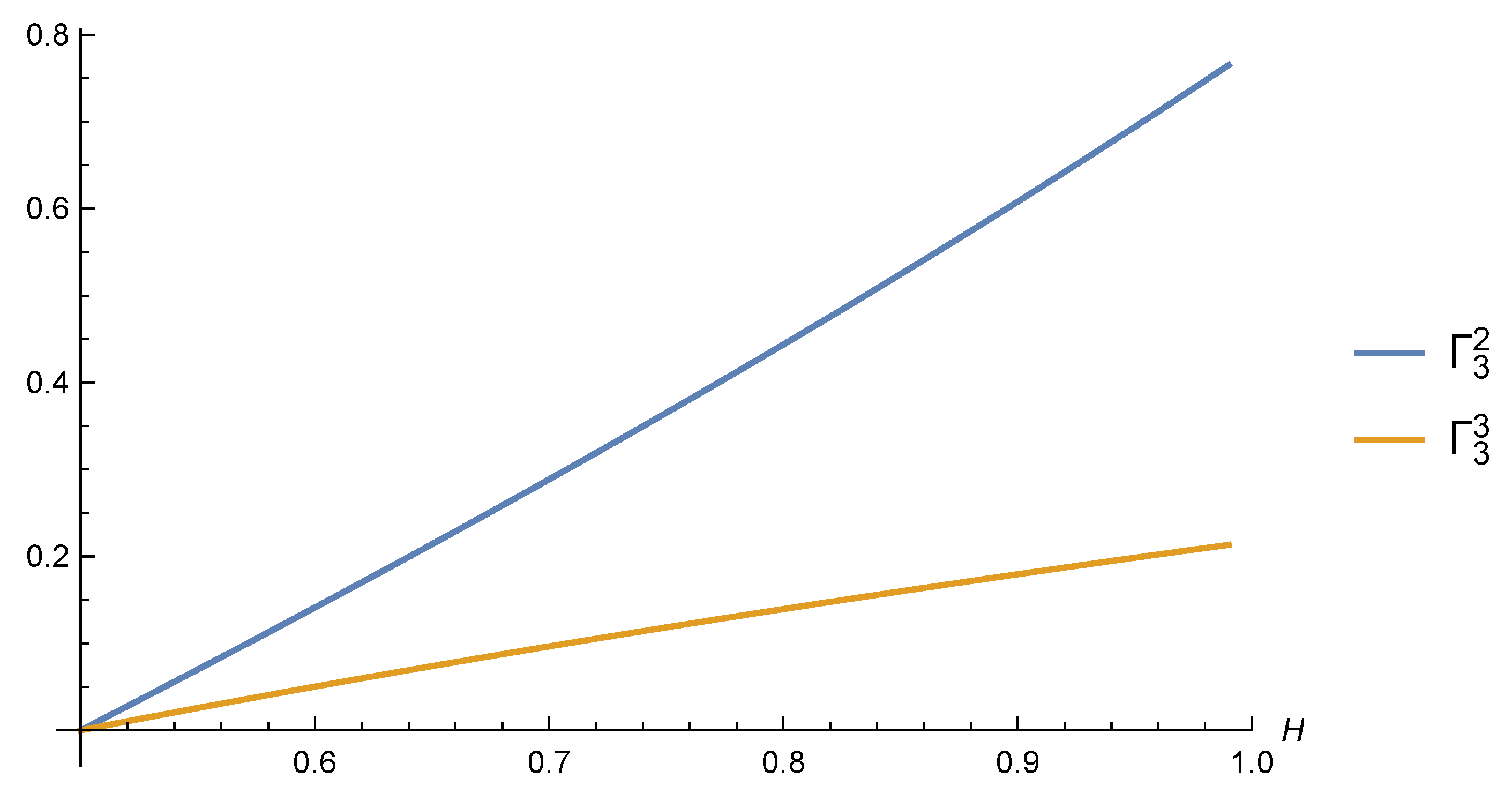
Figure 1 shows the dependence of the coefficients ${\Gamma }_3^2$ and ${\Gamma }_3^3$ on H. It illustrates the theoretical results stated in Propositions 1 and 2, in particular, the positivity and monotonicity of the coefficients, and convergence to theoretical limit values as $H\uparrow 1$.

2.3.2. Case $n=4$

For $n=4$, the system (4) has the following form

$$\begin{array}{c}\left\{\begin{array}{cc}\hfill {\rho }_1& ={\Gamma }_4^2+{\Gamma }_4^3{\rho }_1+{\Gamma }_4^4{\rho }_2,\hfill \\ \hfill {\rho }_2& ={\Gamma }_4^2{\rho }_1+{\Gamma }_4^3+{\Gamma }_4^4{\rho }_1,\hfill \\ \hfill {\rho }_3& ={\Gamma }_4^2{\rho }_2+{\Gamma }_4^3{\rho }_1+{\Gamma }_4^4.\hfill \end{array}\right.\end{array}$$

Therefore,

$$\begin{array}{cc}\hfill {\Gamma }_4^2& =\frac{{\rho }_1+{\rho }_1^2{\rho }_3+{\rho }_1{\rho }_2^2-{\rho }_2{\rho }_3-{\rho }_1^3-{\rho }_1{\rho }_2}{1+2{\rho }_1^2{\rho }_2-{\rho }_2^2-2{\rho }_1^2},\hfill \end{array}$$

(19)

$$\begin{array}{cc}\hfill {\Gamma }_4^3& =\frac{{\rho }_1^2{\rho }_2-{\rho }_2^3+{\rho }_1{\rho }_2{\rho }_3-{\rho }_1^2+{\rho }_2-{\rho }_1{\rho }_3}{1+2{\rho }_1^2{\rho }_2-{\rho }_2^2-2{\rho }_1^2},\hfill \end{array}$$

(20)

$$\begin{array}{cc}\hfill {\Gamma }_4^4& =\frac{{\rho }_1^3+{\rho }_1{\rho }_2^2-2{\rho }_1{\rho }_2+{\rho }_3-{\rho }_1^2{\rho }_3}{1+2{\rho }_1^2{\rho }_2-{\rho }_2^2-2{\rho }_1^2}.\hfill \end{array}$$

(21)

Proposition 3.

For any $H\in (\frac{1}{2},1)$,

$$\begin{array}{c}{\Gamma }_4^2>{\Gamma }_4^3\mathrm{and}{\Gamma }_4^4>0.\end{array}$$

Proof. 

The positivity of the denominator follows from the representation

$$\begin{array}{c}1+2{\rho }_1^2{\rho }_2-{\rho }_2^2-2{\rho }_1^2=(1-{\rho }_2)(1-{\rho }_1^2)+(1-{\rho }_2)({\rho }_2-{\rho }_1^2)\end{array}$$

(22)

and with Corollary 1. Therefore, it suffices to prove the claimed relations for the numerators of ${\Gamma }_4^2$, ${\Gamma }_4^3$, and ${\Gamma }_4^4$.

1. Let us prove that ${\Gamma }_4^2>{\Gamma }_4^3$. The difference between the numerators of ${\Gamma }_4^2$ and ${\Gamma }_4^3$ is equal to

$$\begin{array}{c}({\rho }_1+{\rho }_1^2{\rho }_3+{\rho }_1{\rho }_2^2-{\rho }_2{\rho }_3-{\rho }_1^3-{\rho }_1{\rho }_2)-({\rho }_1^2{\rho }_2-{\rho }_2^3+{\rho }_1{\rho }_2{\rho }_3-{\rho }_1^2+{\rho }_2-{\rho }_1{\rho }_3)\\ =({\rho }_1-{\rho }_2)(1+{\rho }_3)(1-{\rho }_2)+({\rho }_1^2-{\rho }_2^2)(1-{\rho }_1-{\rho }_2+{\rho }_3)>0,\end{array}$$

since ${\rho }_1>{\rho }_2$ and $1-{\rho }_1\ge {\rho }_2-{\rho }_3$ by Statements 1 and 2 of Corollary 1.

2. Finally, the positivity of ${\Gamma }_4^4$ follows from the following representation of its numerator:

$$\begin{array}{c}{\rho }_1^3+{\rho }_1{\rho }_2^2-2{\rho }_1{\rho }_2+{\rho }_3-{\rho }_1^2{\rho }_3={({\rho }_1-{\rho }_2)}^2+(1-{\rho }_1)({\rho }_3-{\rho }_1^2+{\rho }_1{\rho }_3-{\rho }_2^2),\end{array}$$

because ${\rho }_3>{\rho }_1^2$ and ${\rho }_1{\rho }_3>{\rho }_2^2$ by (16), and (13), respectively.    □

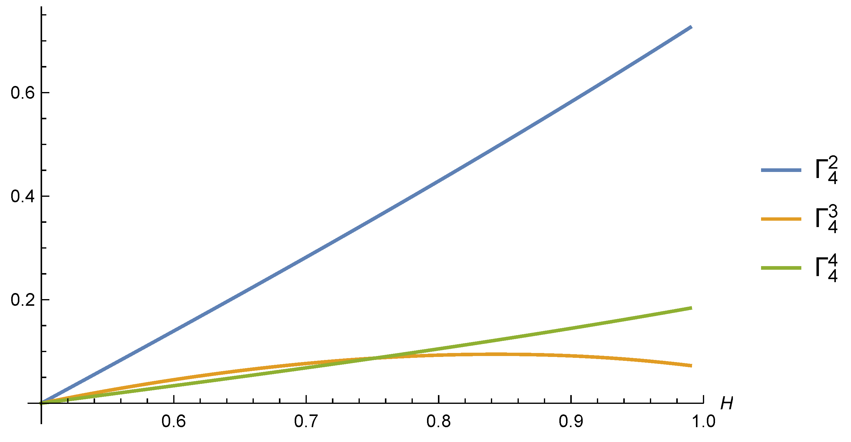
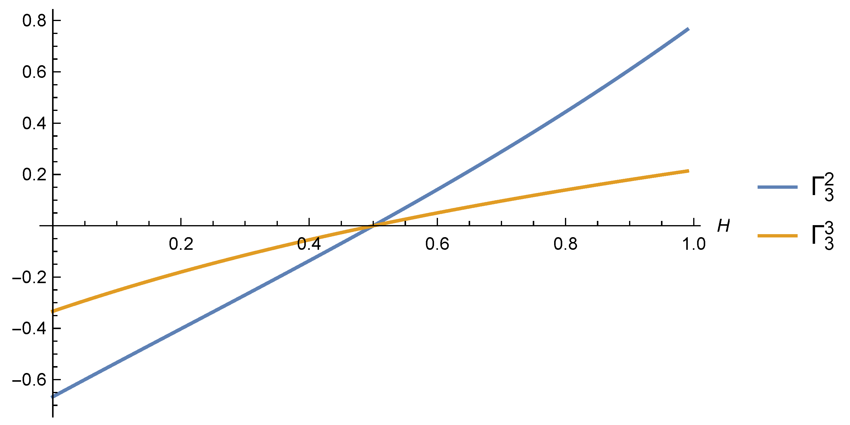
Figure 2 confirms the above proposition. We see that ${\Gamma }_4^2$ is the largest coefficient. However, ${\Gamma }_4^3>{\Gamma }_4^4$ only for $H<0.752281$; for larger H, the order changes.

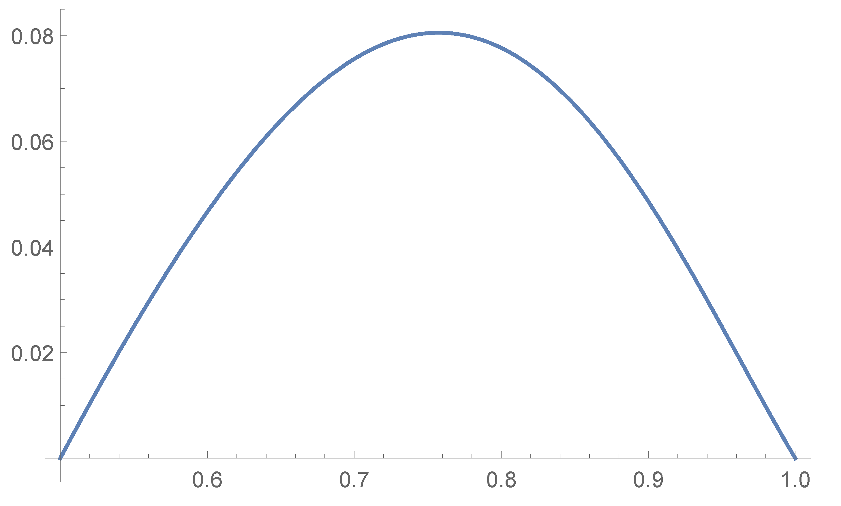
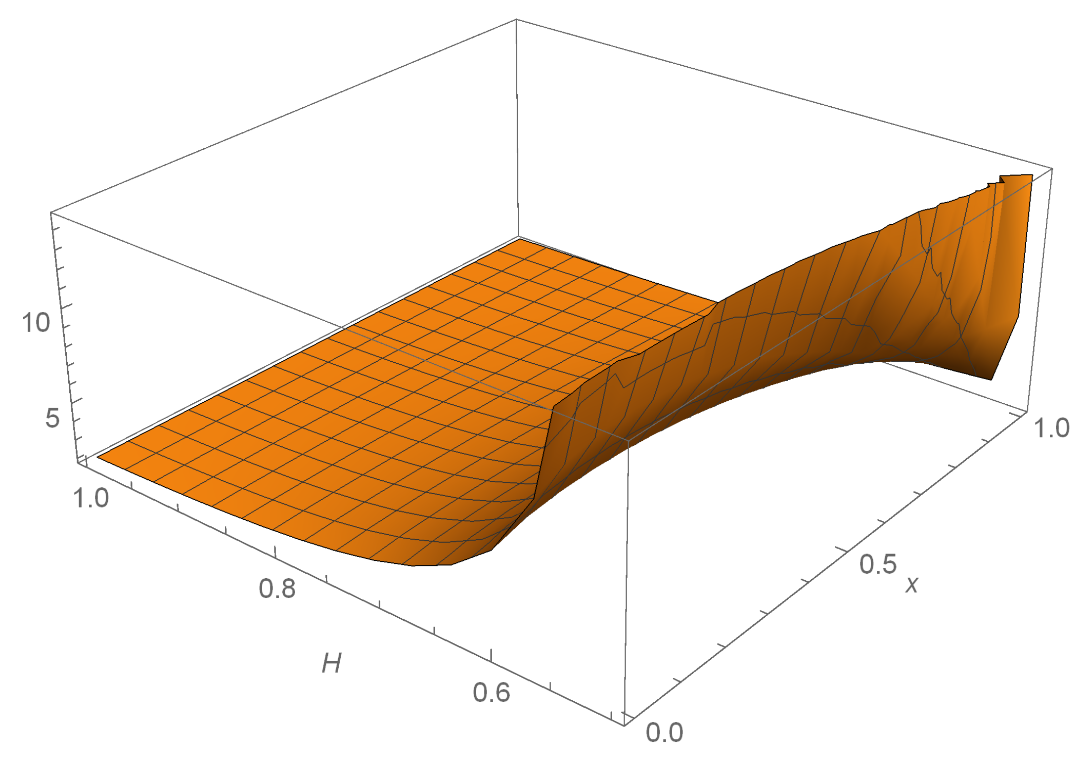
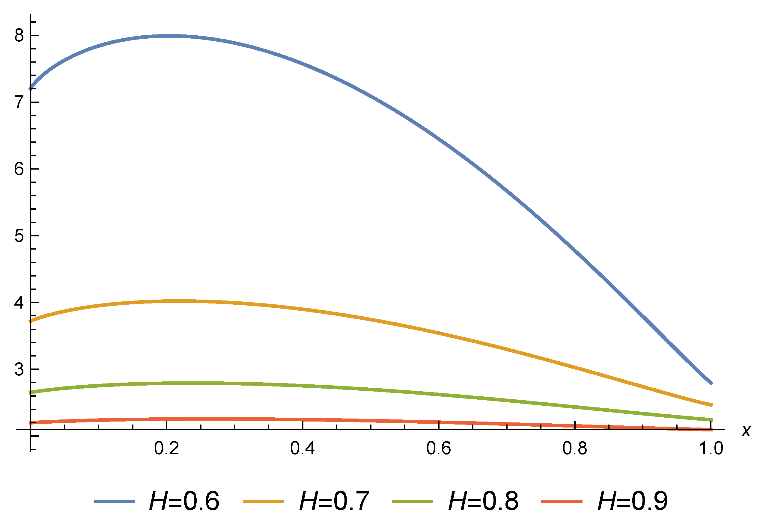
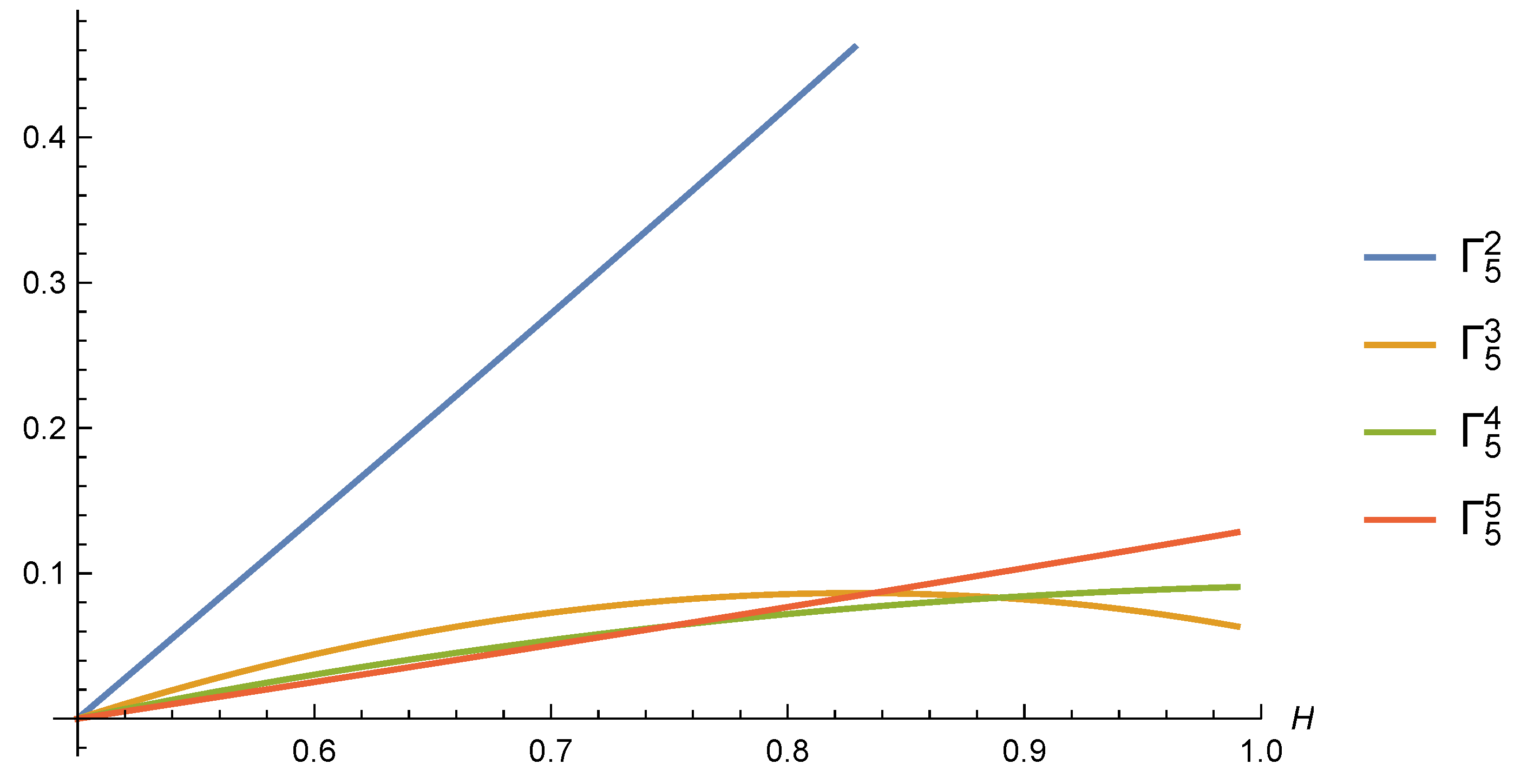
Remark 5.

Consider numerically the relation between ${\Gamma }_4^3$ and ${\Gamma }_4^4$ and the sign of ${\Gamma }_4^3$. One may represent the numerator of ${\Gamma }_4^3$ as follows:

$$\begin{array}{c}{\rho }_1^2{\rho }_2-{\rho }_2^3+{\rho }_1{\rho }_2{\rho }_3-{\rho }_1^2+{\rho }_2-{\rho }_1{\rho }_3=(1-{\rho }_2)({\rho }_2+{\rho }_2^2-{\rho }_1^2-{\rho }_1{\rho }_3).\end{array}$$

(23)

Thus we need to establish that

$$\begin{array}{c}{\rho }_2+{\rho }_2^2-{\rho }_1^2-{\rho }_1{\rho }_3>0.\end{array}$$

(24)

We established this fact numerically since we could not come up with an analytical proof. Figure 3 shows the plot of the left-hand side of (24) that confirms the positivity of ${\Gamma }_4^3$.

However, we can look at (24) from another point of view. Rewrite (24) in the following form:

$$\begin{array}{c}\frac{1+{\rho }_2}{{\rho }_1}>\frac{{\rho }_1+{\rho }_3}{{\rho }_2}.\end{array}$$

The left- and the right-hand sides of this inequality are the values at the points $x=0$ and $x=1$, respectively, of the following function:

$$\begin{array}{cc}\hfill \psi (H,x)& :=\frac{\rho (H,x)+\rho (H,x+2)}{\rho (H,x+1)}\hfill \\ \hfill & =\frac{{(x+3)}^{2H}-2{(x+2)}^{2H}+2{(x+1)}^{2H}-2x^{2H}+{(1-x)}^{2H}}{{(x+2)}^{2H}-2{(x+1)}^{2H}+x^{2H}},x\in [0,1].\hfill \end{array}$$

The graph of the surface $\left\{\psi (H,x),x\in [0,1],H\in (1/2,1)\right\}$ is shown in Figure 4. It was natural to assume that the function $\psi (H,x)$ decreases in x for any H, being at $x=0$ bigger than at $x=1$. However, the function is not monotone for all H. Figure 5 contains two-dimensional plots of $\left\{\psi (H,x),x\in [0,1]\right\}$ for four different values of H: $0.6$, $0.7$, $0.8$ and $0.9$. We observe that $\psi (H,0)>\psi (H,1)$ for each value of H; however, the function $\psi (H,x)$ changes its behavior from increasing to decreasing.

Remark 6.

The unexpected behavior of $\psi (H,x),x\in [0,1]$ (first increasing, then decreasing) is a consequence of the non-standard term ${(1-x)}^{2H}$. For $x\ge 1$, this function decreases in x for any $H>1/2$. Indeed, for $x\ge 1$, it has the form

$$\begin{array}{cc}\hfill \psi (H,x)& =\frac{{(x+3)}^{2H}-2{(x+2)}^{2H}+2{(x+1)}^{2H}-2x^{2H}+{(x-1)}^{2H}}{{(x+2)}^{2H}-2{(x+1)}^{2H}+x^{2H}}\hfill \\ \hfill & =-2+\frac{{(x+3)}^{2H}+{(x-1)}^{2H}-2{(x+1)}^{2H}}{{(x+2)}^{2H}-2{(x+1)}^{2H}+x^{2H}}\hfill \\ \hfill & =-2+\frac{{(1+\frac{2}{x+1})}^{2H}+{(1-\frac{2}{x+1})}^{2H}-2}{{(1+\frac{1}{x+1})}^{2H}+{(1-\frac{1}{x+1})}^{2H}-2}.\hfill \end{array}$$

Write $y=\frac{1}{x+1}\in (0,\frac{1}{2}]$. It is sufficient to prove that the function

$$\begin{array}{c}\eta (H,y)=\frac{{(1+2y)}^{2H}+{(1-2y)}^{2H}-2}{{(1+y)}^{2H}+{(1-y)}^{2H}-2},y\in (0,\frac{1}{2}],\end{array}$$

increases in y for any $H\in (\frac{1}{2},1)$. However, for $y<\frac{1}{2}$,

$$\begin{array}{c}{(1+y)}^{2H}+{(1-y)}^{2H}-2=\sum _{k=0}^{\infty }{c}_k{y}^{2k+2}\end{array}$$

and

$$\begin{array}{c}\hfill {(1+2y)}^{2H}+{(1-2y)}^{2H}-2=\sum _{k=0}^{\infty }{c}_k{\left(2y\right)}^{2k+2},\end{array}$$

where

$$\begin{array}{c}\hfill c_k=\frac{4H(2H-1)(2H-2)\dots (2H-2k-1)}{(2k+2)!}=\frac{2{\left(2H\right)}_{2k+2}}{(2k+2)!},k=0,1,2,\dots \end{array}$$

(here ${\left(x\right)}_n=x(x-1)\dots (x-n+1)$ is the Pochhammer symbol). The monotonicity of $\eta (H,y)$ for $y\in (0,\frac{1}{2}]$ can be proved by differentiation. Then

$$\begin{array}{c}\eta (H,y)=\frac{{\sum }_{k=0}^{\infty }{c}_k{2}^{2k+2}{y}^{2k}}{{\sum }_{k=0}^{\infty }{c}_k{y}^{2k}},\end{array}$$

(25)

and hence, the partial derivative equals

$$\begin{array}{cc}\hfill & \frac{\partial }{\partial y}\eta (H,y)\hfill \\ \hfill & ={\left(\sum _{k=0}^{\infty }{c}_k{y}^{2k}\right)}^{-2}\left(\sum _{k=1}^{\infty }{c}_k{2}^{2k+2}2k{y}^{2k-1}\sum _{l=0}^{\infty }{c}_l{y}^{2l}-\sum _{k=1}^{\infty }{c}_{k}2k{y}^{2k-1}\sum _{l=0}^{\infty }{c}_l{2}^{2l+2}{y}^{2l}\right)\hfill \\ \hfill & ={\left(\sum _{k=0}^{\infty }{c}_k{y}^{2k}\right)}^{-2}\sum _{k=1}^{\infty }\sum _{l=0}^{\infty }{c}_k{c}_l·2k\left(2^{2k+2}-2^{2l+2}\right)y^{2k+2l-1}.\hfill \end{array}$$

By rearranging the double sum in the numerator, we obtain the expression

$$\begin{array}{c}\frac{\partial }{\partial y}\eta (H,y)={\left(\sum _{k=0}^{\infty }{c}_k{y}^{2k}\right)}^{-2}\sum _{k=1}^{\infty }\sum _{l=0}^k{c}_k{c}_l(2k-2l)\left(2^{2k+2}-2^{2l+2}\right)y^{2k+2l-1},\end{array}$$

which is clearly positive. Thus for any $H\in (\frac{1}{2},1)$, $\eta (H,y)$ is increasing as a function of $y\in (0,\frac{1}{2})$.

Let us try to establish a bit more. We can represent $\eta (H,y)$ in the following form:

$$\begin{array}{c}\eta (H,y)=\frac{{\sum }_{k=0}^{\infty }{c}_k{2}^{2k+2}{y}^{2k}}{{\sum }_{k=0}^{\infty }{c}_k{y}^{2k}}=\sum _{k=0}^{\infty }{b}_k{y}^{2k},\end{array}$$

where the coefficients $b_k$ can be found successively from the following equations:

$$\begin{array}{cc}\hfill 2^2{c}_0& =c_0{b}_0,\hfill \\ \hfill 2^4{c}_1& =c_0{b}_1+c_1{b}_0,\hfill \\ \hfill 2^6{c}_2& =c_0{b}_2+c_1{b}_1+c_2{b}_0,\hfill \\ \hfill 2^8{c}_3& =c_0{b}_3+c_1{b}_2+c_2{b}_1+c_3{b}_0,\hfill \\ \hfill & \cdots \hfill \end{array}$$

Let us find the first few coefficients: $b_0=2^2=4$,

$$\begin{array}{cc}\hfill b_1& =\frac{2^4{c}_1-2^2{c}_1}{c_0}=\frac{(2^4-2^2)\frac{(2H-1)(2H-2)(2H-3)}{4!}}{\frac{(2H-1)}{2!}}=(2H-2)(2H-3),\hfill \\ \hfill b_2& =\frac{(2^6-2^2)c_2-c_1{b}_1}{c_0}\hfill \\ \hfill & =\frac{60\frac{(2H-1)(2H-2)(2H-3)(2H-4)(2H-5)}{6!}-\frac{(2H-1){(2H-2)}^2{(2H-3)}^2}{4!}}{\frac{(2H-1)}{2!}}\hfill \\ \hfill & =\frac{2!(2H-2)(2H-3)}{4!}\left(2(2H-4)(2H-5)-(2H-2)(2H-3)\right)\hfill \\ \hfill & =\frac{1}{6}(2H-2)(2H-3)(2H^2-13H+17).\hfill \end{array}$$

It is easy to see that $b_0$, $b_1$, and $b_2$ are positive for $H\in (\frac{1}{2},1)$. We believe that $b_k>0$ for all k. However, the proof of this fact remains an open problem.

Proposition 4.

$$\begin{array}{cc}\hfill \underset{H\uparrow 1}{lim}{\Gamma }_4^2& =\frac{531{log}^{2}4+72{log}^{2}6+51{log}^{2}9-384{log}^{2}12+108{log}^{2}18}{96{log}^{2}12-640{log}^{2}2-51{log}^{2}9}\approx 0.742250,\hfill \\ \hfill \underset{H\uparrow 1}{lim}{\Gamma }_4^3& =\frac{48log2-15log9}{16log2-3log9}\approx 0.069508,\hfill \\ \hfill \underset{H\uparrow 1}{lim}{\Gamma }_4^4& =\frac{108{log}^{2}18-364{log}^{2}2-216log2log9-81{log}^{2}9}{96{log}^{2}12-640{log}^{2}2-51{log}^{2}9}\approx 0.188242.\hfill \end{array}$$

Remark 7.

Obviously, the sum of the limits of the coefficients is 1, as expected.

Proof 

(Sketch of proof). The proof is straightforward. Substituting ${\rho }_1=2^{2H-1}-1$, ${\rho }_2=\frac{1}{2}\left(3^{2H}-2^{2H+1}+1\right)$, and ${\rho }_3=\frac{1}{2}\left(4^{2H}-2·3^{2H}+2^{2H}\right)$ into (19)–(21), and simplifying the resulting expressions, we obtain

$$\begin{array}{cc}\hfill {\Gamma }_4^2& =\frac{2-7·4^H+4^{3H+1}+6^{2H+1}-4·9^H-2^{4H+3}·9^H+2·9^{2H}+4^{4H}+{18}^{2H}}{2\left(-2^{6H+1}+2·9^H+3·2^{4H}-9^{2H}+{12}^{2H}-1\right)},\hfill \\ \hfill {\Gamma }_4^3& =\frac{-2^{2H+1}+4^{2H+1}-2^{2H+1}·9^H-{64}^H+9^{2H}-1}{2\left(2^{2H+1}+9^H-{16}^H-1\right)},\hfill \\ \hfill {\Gamma }_4^4& =\frac{-3·2^{4H+1}+4^H+8^{2H+1}+4·9^H-2^{2H+1}·9^H-2^{4H+1}·9^H-2·9^{2H}-4^{4H}+{18}^{2H}-2}{2\left(-2^{6H+1}+2·9^H+3·2^{4H}-9^{2H}+{12}^{2H}-1\right)}\hfill \end{array}$$

(for ${\Gamma }_4^3$, we first cancel out the factor $1-{\rho }_2$, see (22) and (23)). Then applying l’Hôpital’s rule (twice), we arrive at the claimed limits by simple algebra.    □

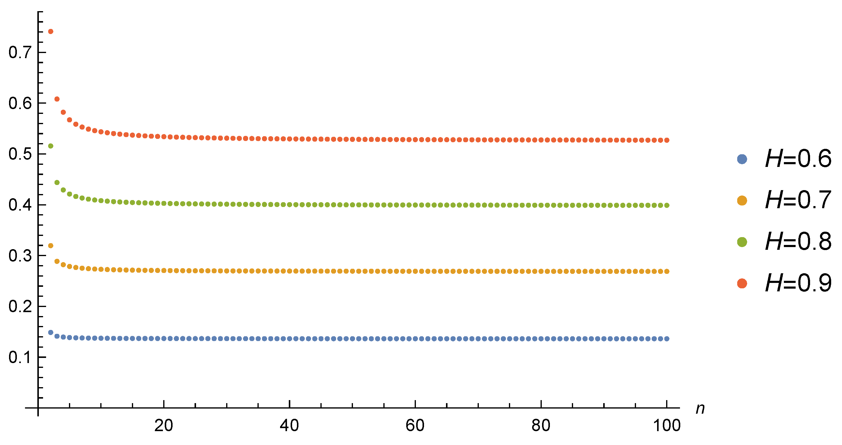
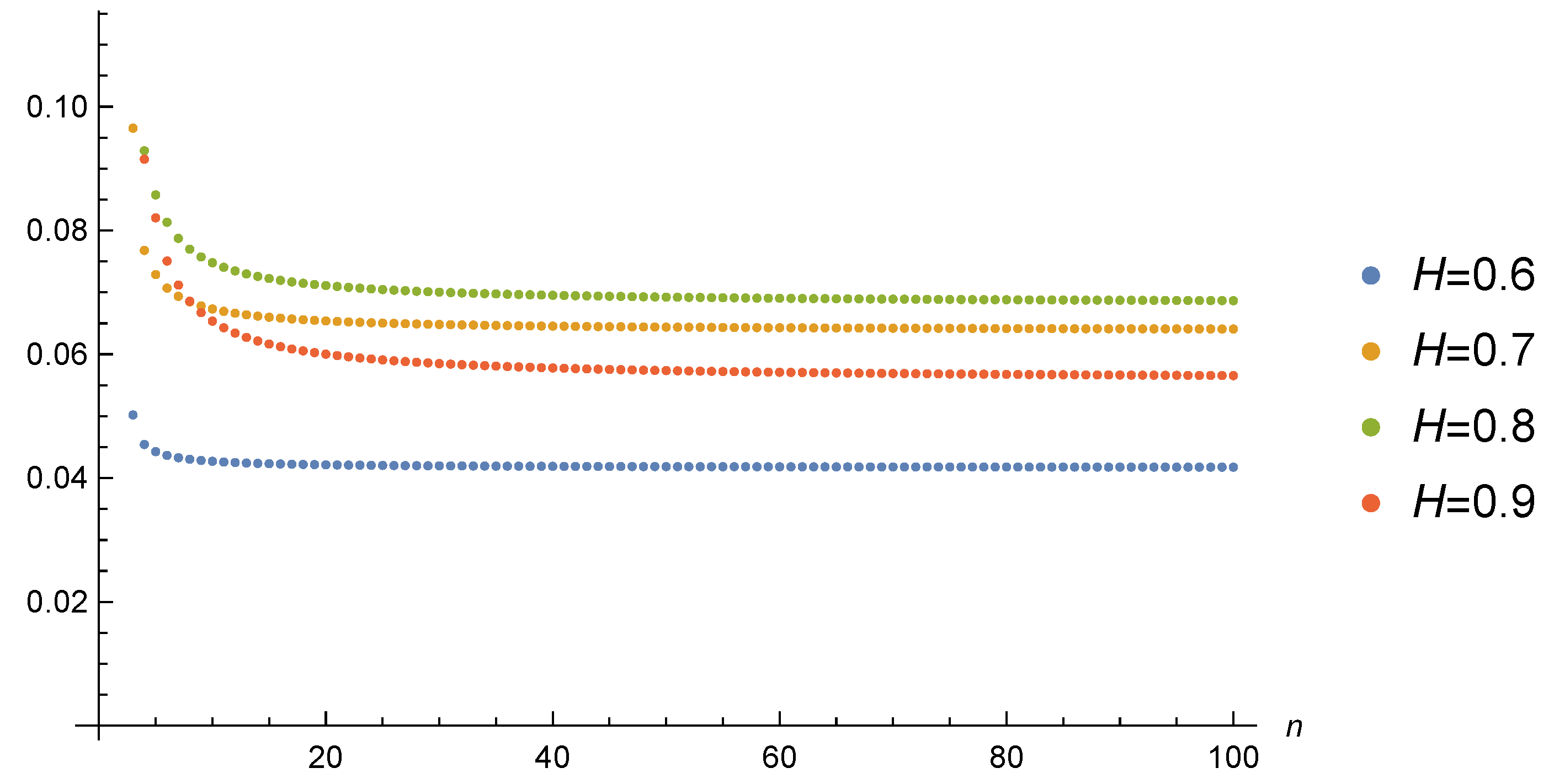
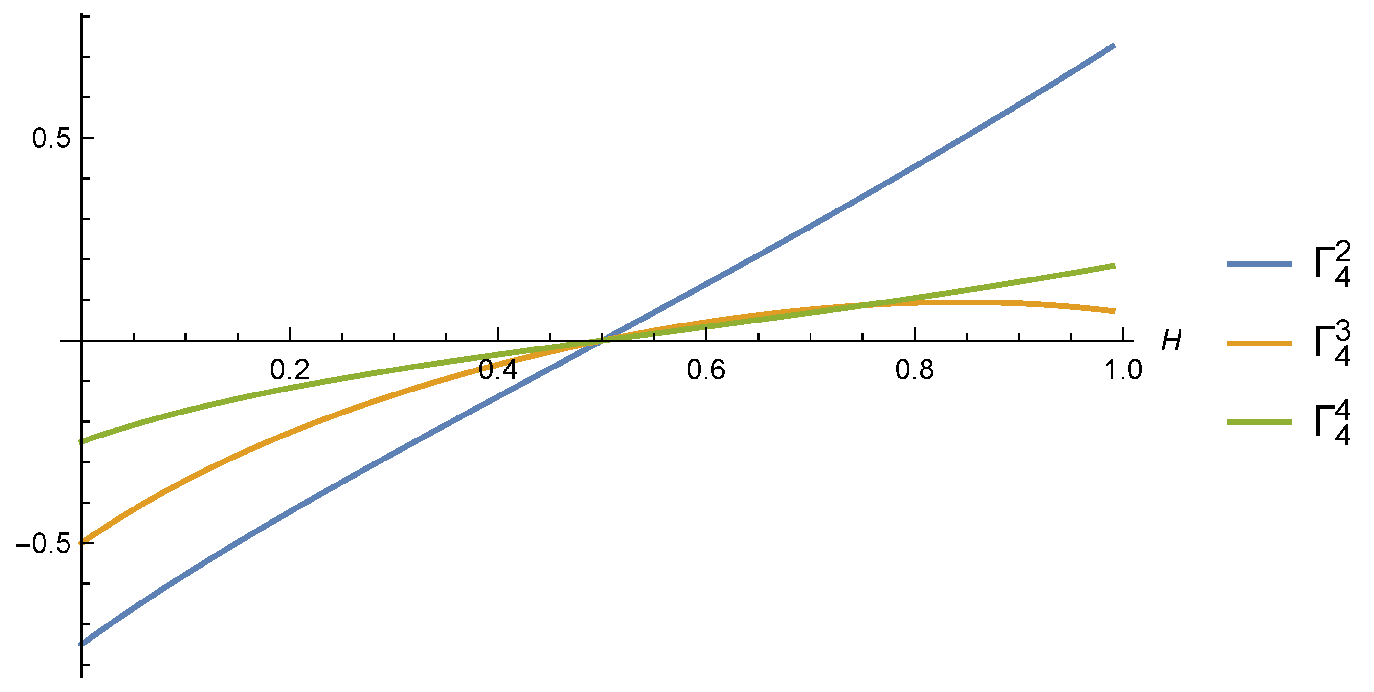
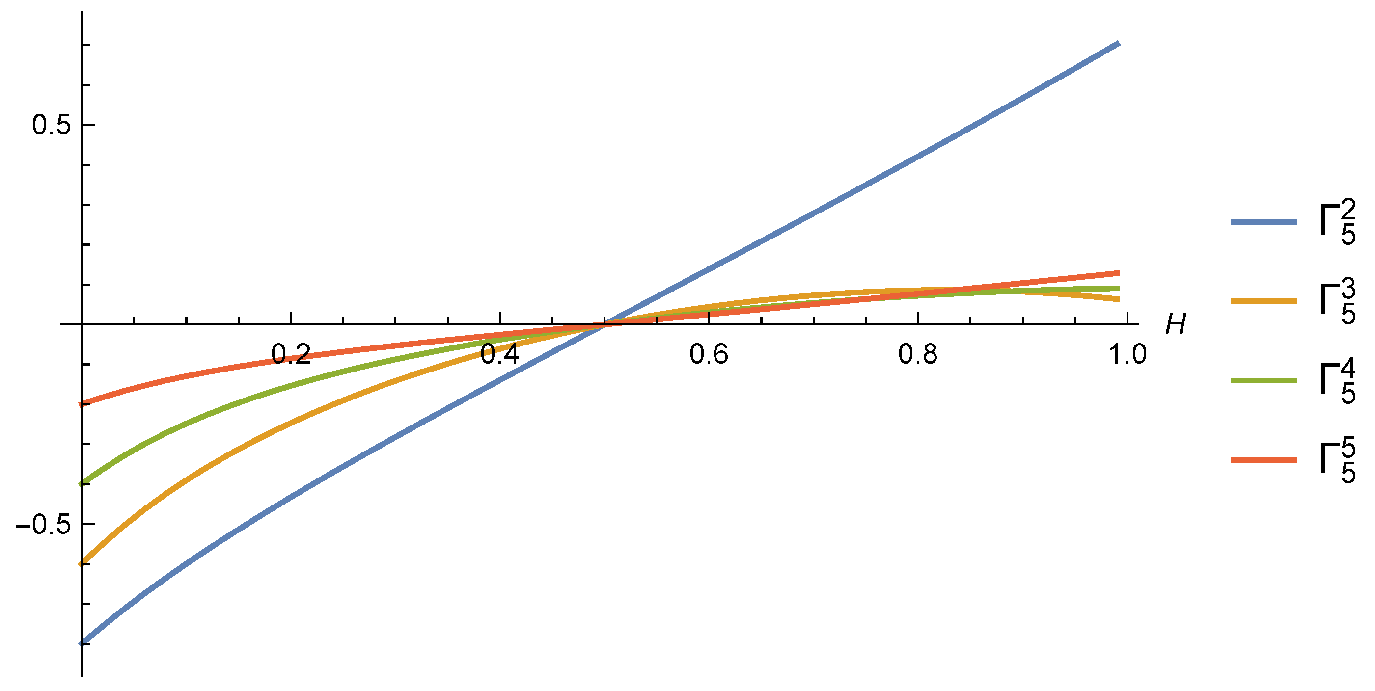
Remark 8.

For $n=5$, we present the graphical results only; see Figure 6. The situation here is more complicated compared to the case $n=4$. The first coefficient ${\Gamma }_5^2$ is still the largest; however, the order of three other coefficients changes several times depending on H. In particular, for H close to 1/2, these coefficients are decreasing, but for H close to 1, they are increasing.

2.4. Recurrence Relations for the Coefficients

In general, there are several ways to obtain (4). For example, we can consider the coefficients ${\Gamma }_n^k$ as a result of minimizing the value of the quadratic form

$$\begin{array}{c}\mathbb{E}{({\Delta }_1-\sum _{k=2}^n{\alpha }_k{\Delta }_k)}^2.\end{array}$$

Evidently, differentiation leads again to the system (4). We can look for the coefficients with the help of the inverse matrix $A^{-1}$, where A is from (5). However, calculating the entries of the inverse matrix is as difficult as calculating the determinants. It is possible to avoid determinants using the properties of fGn. More precisely, we propose a recurrence method to calculate the coefficients ${\Gamma }_n^k$ successively, starting with ${\Gamma }_2^2={\rho }_1=2^{2H-1}-1$.

Proposition 5.

The following relations hold true:

$$\begin{array}{cc}\hfill {\Gamma }_{n+1}^{n+1}& =\frac{{\rho }_n-{\sum }_{k=2}^n{\Gamma }_n^k{\rho }_{n+1-k}}{1-{\sum }_{k=2}^n{\Gamma }_n^k{\rho }_{k-1}},n\ge 2,\hfill \end{array}$$

(26)

$$\begin{array}{cc}\hfill {\Gamma }_{n+1}^k& ={\Gamma }_n^k-{\Gamma }_{n+1}^{n+1}{\Gamma }_n^{n-k+2},n\ge 2,2\le k\le n.\hfill \end{array}$$

(27)

Proof. 

In order to prove (26) and (27), we use the theorem on normal correlation as well as the independence of ${\Delta }_{n+1}-\mathbb{E}\left({\Delta }_{n+1}\mid {\Delta }_2,\cdots ,{\Delta }_n\right)$ and any of ${\Delta }_k,2\le k\le n$. We get

$$\begin{array}{c}\mathbb{E}\left({\Delta }_1\mid {\Delta }_2,\cdots ,{\Delta }_n,{\Delta }_{n+1}\right)=\sum _{k=2}^n{\tilde{\Gamma }}_n^k{\Delta }_k+{\Gamma }_{n+1}^{n+1}\left({\Delta }_{n+1}-\mathbb{E}\left({\Delta }_{n+1}\mid {\Delta }_2,\cdots ,{\Delta }_n\right)\right),\end{array}$$

(28)

where ${\tilde{\Gamma }}_n^k$, $2\le k\le n$, are some constants. Now we take the conditional expectation $\mathbb{E}\left(·\mid {\Delta }_2,\dots ,{\Delta }_n\right)$ on both sides of (28) to obtain

$$\begin{array}{c}\mathbb{E}\left({\Delta }_1\mid {\Delta }_2,\dots ,{\Delta }_n\right)=\sum _{k=2}^n{\tilde{\Gamma }}_{n+1}^k{\Delta }_k.\end{array}$$

Comparing this equality with (3), and taking into account that the increments ${\Delta }_k$, $2\le k\le n$ are linearly independent, we conclude that

$$\begin{array}{c}\sum _{k=2}^n{\tilde{\Gamma }}_{n+1}^k{\Delta }_k=\sum _{k=2}^n{\Gamma }_n^k{\Delta }_k.\end{array}$$

Now we insert this equality into (28) and see

$$\begin{array}{c}\mathbb{E}\left({\Delta }_1\mid {\Delta }_2,\dots ,{\Delta }_n,{\Delta }_{n+1}\right)=\sum _{k=2}^n{\Gamma }_n^k{\Delta }_k+{\Gamma }_{n+1}^{n+1}\left({\Delta }_{n+1}-\mathbb{E}\left({\Delta }_{n+1}\mid {\Delta }_2,\dots ,{\Delta }_n\right)\right).\end{array}$$

(29)

After multiplying both sides of the last equality by $\left({\Delta }_{n+1}-\mathbb{E}\left({\Delta }_{n+1}\mid {\Delta }_2,\dots ,{\Delta }_n\right)\right)$ and taking expectations, we arrive at

$$\begin{array}{c}\mathbb{E}\left({\Delta }_1\left({\Delta }_{n+1}-\mathbb{E}\left({\Delta }_{n+1}\mid {\Delta }_2,\dots ,{\Delta }_n\right)\right)\right)={\Gamma }_{n+1}^{n+1}\mathbb{E}{\left({\Delta }_{n+1}-\mathbb{E}\left({\Delta }_{n+1}\mid {\Delta }_2,\dots ,{\Delta }_n\right)\right)}^2.\end{array}$$

It follows from the stationarity of the increments that the indices $n+1$ and 1 of the last equality play symmetric roles, i.e., they are equivalent to

$$\begin{array}{c}\mathbb{E}\left({\Delta }_{n+1}\left({\Delta }_1-\mathbb{E}\left({\Delta }_1\mid {\Delta }_2,\dots ,{\Delta }_n\right)\right)\right)={\Gamma }_{n+1}^{n+1}\mathbb{E}{\left({\Delta }_1-\mathbb{E}\left({\Delta }_1\mid {\Delta }_2,\dots ,{\Delta }_n\right)\right)}^2.\end{array}$$

From this, we conclude that

$$\begin{array}{cc}\hfill {\Gamma }_{n+1}^{n+1}& =\frac{\mathbb{E}\left({\Delta }_{n+1}\left({\Delta }_1-\mathbb{E}\left({\Delta }_1\mid {\Delta }_2,\dots ,{\Delta }_n\right)\right)\right)}{\mathbb{E}{\left({\Delta }_1-\mathbb{E}\left({\Delta }_1\mid {\Delta }_2,\dots ,{\Delta }_n\right)\right)}^2}\hfill \\ \hfill & =\frac{{\rho }_n-{\sum }_{k=2}^n{\Gamma }_n^k{\rho }_{n+1-k}}{1-{\sum }_{k=2}^n{\Gamma }_n^k{\rho }_{k-1}}.\hfill \end{array}$$

Thus, the relation (26) is proved.

Using again the symmetry of the stationary increments, it is not hard to see that

$$\begin{array}{c}\mathbb{E}\left({\Delta }_{n+1}\mid {\Delta }_2,\dots ,{\Delta }_n\right)=\sum _{k=2}^n{\Gamma }_n^{n-k+2}{\Delta }_k.\end{array}$$

Therefore, we obtain from (29) that

$$\begin{array}{cc}\hfill \mathbb{E}\left({\Delta }_1\mid {\Delta }_2,\dots ,{\Delta }_n,{\Delta }_{n+1}\right)& =\sum _{k=2}^n{\Gamma }_n^k{\Delta }_k+{\Gamma }_{n+1}^{n+1}{\Delta }_{n+1}-{\Gamma }_{n+1}^{n+1}\sum _{k=2}^n{\Gamma }_n^{n-k+2}{\Delta }_k\hfill \\ \hfill & =\sum _{k=2}^n\left({\Gamma }_n^k-{\Gamma }_{n+1}^{n+1}{\Gamma }_n^{n-k+2}\right){\Delta }_k+{\Gamma }_{n+1}^{n+1}{\Delta }_{n+1},\hfill \end{array}$$

and (27) follows.    □

2.5. Positivity of ${\Gamma }_n^2$

We conjecture that all coefficients ${\Gamma }_n^k$, $2\le k\le n$ are positive. However, analytically, we can prove only the positivity of the leading coefficient, ${\Gamma }_n^2$.

Proposition 6.

For all $n\ge 1$, ${\Gamma }_{n+1}^2>0$.

Proof. 

From the stationarity of the increments, it follows that

$$\begin{array}{c}\mathbb{E}\left({\Delta }_2\mid {\Delta }_3,\dots ,{\Delta }_{n+1}\right)=\sum _{k=3}^{n+1}{\Gamma }_n^{k-1}{\Delta }_k.\end{array}$$

Similar to (29),

$$\begin{array}{c}\mathbb{E}\left({\Delta }_1\mid {\Delta }_2,\dots ,{\Delta }_n,{\Delta }_{n+1}\right)={\tilde{\Gamma }}_{n+1}^2\left({\Delta }_2-\mathbb{E}\left({\Delta }_2\mid {\Delta }_3,\dots ,{\Delta }_{n+1}\right)\right)+\sum _{k=3}^{n+1}{\Gamma }_{n+1}^k{\Delta }_k,\end{array}$$

and so

$$\begin{array}{c}{\Gamma }_{n+1}^2={\tilde{\Gamma }}_{n+1}^2=\frac{\mathbb{E}\left(\left({\Delta }_2-\mathbb{E}\left({\Delta }_2\mid {\Delta }_3,\dots ,{\Delta }_{n+1}\right)\right){\Delta }_1\right)}{\mathbb{E}{\left({\Delta }_2-\mathbb{E}\left({\Delta }_2\mid {\Delta }_3,\dots ,{\Delta }_{n+1}\right)\right)}^2}.\end{array}$$

It remains to prove the positivity of the numerator

$$\begin{array}{c}\mathbb{E}\left(\left({\Delta }_2-\mathbb{E}\left({\Delta }_2\mid {\Delta }_3,\dots ,{\Delta }_{n+1}\right)\right){\Delta }_1\right)={\rho }_1-\sum _{k=3}^{n+1}{\Gamma }_n^{k-1}{\rho }_{k-1}.\end{array}$$

However, we know from (4) that

$$\begin{array}{c}{\rho }_1=\sum _{k=2}^n{\Gamma }_n^k{\rho }_{k-2}.\end{array}$$

Therefore,

$$\begin{array}{c}{\rho }_1-\sum _{k=3}^{n+1}{\Gamma }_n^{k-1}{\rho }_{k-1}=\sum _{k=2}^n{\Gamma }_n^k{\rho }_{k-2}-\sum _{k=2}^n{\Gamma }_n^k{\rho }_k=\sum _{k=2}^n{\Gamma }_n^k\left({\rho }_{k-2}-{\rho }_k\right)>0,\end{array}$$

since the sequence ${\rho }_k$ is decreasing, see Corollary 1.    □

3. Numerical Results

3.1. Properties of Coefficients: Positivity and (non)monotonicity

In this section, we compute numerically the coefficients ${\Gamma }_n^k$ for various values of H. In

Table 1. Coefficients ${\Gamma }_n^k$ for $H=0.51$.

$\mathit{n}\setminus \mathit{k}$	2	3	4	5	6	7	8	9	10
2	0.01396
3	0.01389	0.00521
4	0.01387	0.00516	0.00339
5	0.01386	0.00515	0.00336	0.00253
6	0.01386	0.00514	0.00335	0.00250	0.00201
7	0.01385	0.00514	0.00334	0.00249	0.00199	0.00167
8	0.01385	0.00514	0.00334	0.00248	0.00198	0.00165	0.00143
9	0.01385	0.00513	0.00334	0.00248	0.00198	0.00165	0.00142	0.00125
10	0.01385	0.00513	0.00333	0.00248	0.00198	0.00164	0.00141	0.00124	0.00111

,

Table 2. Coefficients ${\Gamma }_n^k$ for $H=0.6$.

$\mathit{n}\setminus \mathit{k}$	2	3	4	5	6	7	8	9	10
2	0.14870
3	0.14123	0.05020
4	0.13954	0.04542	0.03383
5	0.13868	0.04427	0.03031	0.02522
6	0.13817	0.04366	0.02942	0.02243	0.02013
7	0.13784	0.04329	0.02893	0.02170	0.01781	0.01675
8	0.13760	0.04303	0.02862	0.02129	0.01719	0.01477	0.01434
9	0.13742	0.04285	0.02840	0.02102	0.01683	0.01423	0.01262	0.01254
10	0.13728	0.04271	0.02824	0.02083	0.01660	0.01391	0.01214	0.01101	0.01114

,

Table 3. Coefficients ${\Gamma }_n^k$ for $H=0.7$.

$\mathit{n}\setminus \mathit{k}$	2	3	4	5	6	7	8	9	10
2	0.31951
3	0.28867	0.09652
4	0.28207	0.07677	0.06840
5	0.27860	0.07288	0.05409	0.05074
6	0.27654	0.07069	0.05114	0.03946	0.04048
7	0.27518	0.06936	0.04942	0.03708	0.03117	0.03366
8	0.27421	0.06846	0.04835	0.03566	0.02917	0.02573	0.02881
9	0.27348	0.06782	0.04762	0.03476	0.02796	0.02401	0.02191	0.02518
10	0.27292	0.06733	0.04708	0.03413	0.02718	0.02295	0.02039	0.01907	0.02237

,

Table 4. Coefficients ${\Gamma }_n^k$ for $H=0.8$.

$\mathit{n}\setminus \mathit{k}$	2	3	4	5	6	7	8	9	10
2	0.51572
3	0.44379	0.13947
4	0.42915	0.09287	0.10500
5	0.42108	0.08574	0.07202	0.07684
6	0.41637	0.08132	0.06676	0.05103	0.06130
7	0.41325	0.07873	0.06336	0.04690	0.04010	0.05089
8	0.41103	0.07698	0.06132	0.04414	0.03668	0.03291	0.04352
9	0.40938	0.07573	0.05993	0.04246	0.03435	0.02999	0.02790	0.03801
10	0.40810	0.07479	0.05892	0.04130	0.03292	0.02796	0.02534	0.02420	0.03373

,

Table 5. Coefficients ${\Gamma }_n^k$ for $H=0.9$.

$\mathit{n}\setminus \mathit{k}$	2	3	4	5	6	7	8	9	10
2	0.74110
3	0.60809	0.17948
4	0.58213	0.09152	0.14465
5	0.56714	0.08204	0.08433	0.10362
6	0.55857	0.07506	0.07754	0.05671	0.08272
7	0.55290	0.07118	0.07223	0.05156	0.04445	0.06852
8	0.54889	0.06858	0.06921	0.04734	0.04028	0.03617	0.05851
9	0.54590	0.06673	0.06716	0.04492	0.03675	0.03266	0.03049	0.05105
10	0.54359	0.06535	0.06568	0.04326	0.03472	0.02962	0.02747	0.02633	0.04527

and

Table 6. Coefficients ${\Gamma }_n^k$ for $H=0.99$.

$\mathit{n}\setminus \mathit{k}$	2	3	4	5	6	7	8	9	10
2	0.97247
3	0.76506	0.21328
4	0.72588	0.07275	0.18368
5	0.70233	0.06342	0.09059	0.12824
6	0.68917	0.05413	0.08408	0.05617	0.10262
7	0.68047	0.04937	0.07696	0.05159	0.04422	0.08474
8	0.67435	0.04617	0.07323	0.04602	0.04065	0.03555	0.07228
9	0.66979	0.04393	0.07067	0.04312	0.03604	0.03265	0.02980	0.06299
10	0.66628	0.04227	0.06885	0.04111	0.03363	0.02870	0.02735	0.02560	0.05582

, the results for $H=0.51$, $0.6$, $0.7$, $0.8$, $0.9$, and $0.99$ are listed for $2\le n\le 10$.

Observe the following:

1.

All coefficients are positive.

2.

The first coefficient in each row is the largest, i.e., ${\Gamma }_n^2>{\Gamma }_n^k$ for any $3\le k\le n$. Moreover, often it is substantially larger than any other coefficient in the row.

3.

The conjecture concerning the monotonicity of coefficients (decrease along each row) does not hold in general. If we take sufficiently large values of H, for example $H=0.9$, we see that the coefficient ${\Gamma }_n^3$ is always less than ${\Gamma }_4$. Moreover, the last coefficient ${\Gamma }_n^n$ is bigger than ${\Gamma }_n^{n-1}$ for sufficiently large H.

4.

The monotonicity along each column holds, i.e., ${\Gamma }_n^k>{\Gamma }_{n+1}^k$ for fixed k. Figure 7 and Figure 8 illustrate the dependence of ${\Gamma }_n^k$ of n for $k=2,3$ and for various H.

5.

The limiting distribution of the coefficients as $H\uparrow 1$ is not uniform.

6.

It immediately follows from (27) that the coefficients satisfy the following relation:

$$\begin{array}{c}{\Gamma }_{n+1}^{k+1}={\Gamma }_n^{k+1}-{\Gamma }_{n+1}^{n+1}{\Gamma }_n^{n-k+1},\end{array}$$

whence

$$\begin{array}{c}{\Gamma }_{n+1}^{k+1}-{\Gamma }_{n+1}^k={\Gamma }_n^{k+1}-{\Gamma }_n^k-{\Gamma }_{n+1}^{n+1}\left({\Gamma }_n^{n-k+1}-{\Gamma }_n^{n-k+2}\right).\end{array}$$

The second of these relations makes us expect that knowing that the coefficients decrease in k for n fixed and that the last coefficient ${\Gamma }_{n+1}^{n+1}$ is positive, we can prove that they decrease in k for $n⇝n+1$ by induction. Unfortunately, if we take $n=3$ as the start of the induction, we see that such a relation holds only if $k=2$, and indeed, ${\Gamma }_4^2>{\Gamma }_4^3$ as we know from Proposition 3. However, the relation between ${\Gamma }_4^3$ and ${\Gamma }_4^4$ is not so stable and depends on H; see Figure 2. Therefore, we cannot state that ${\Gamma }_4^3>{\Gamma }_4^4$.

3.2. Comparison of the Methods: Computation Time

Let us compare the two methods in terms of computation time. The first method (solving the system of equations) was realized using the R function solve(). We considered two problems:

1.

For fixed n, compute the coefficients ${\Gamma }_n^k$, $2\le k\le n$, i.e., compute the nth row of the matrix.

2.

Compute the whole triangular array $\left\{{\Gamma }_m^k\mid 2\le m\le n,2\le k\le m\right\}$. This requires solving $(n-1)$ systems of equations.

The second method (recurrence relations) always gives us the whole array of coefficients, which can be considered an advantage.

Let us mention that both methods give exactly the same values of the coefficients.

We also compared the time needed for computation on an Intel Core i3-8145U processor by each method. The results are shown in

Table 7. Computation time.

n	100	500	1000	2000
System method (last row)	0.02 s	0.20 s	0.51 s	3.10 s
System method (whole matrix)	0.17 s	16.46 s	2.27 min	21.78 min
Recurrence method	0.04 s	0.19 s	0.48 s	1.83 s

. Observe that the recurrence method is always faster, especially for large n, if we need to compute the whole matrix. It takes less than 2 s for $n=2000$, while solving all systems of equations takes more that 21 min. Moreover, for large n the recurrence method is even faster than the calculation of a single row of the matrix, which requires solving only one system of equations.

3.3. Remarks on the Case $H<\frac{1}{2}$

In this paper, we mainly focus on the case $H>\frac{1}{2}$ (the case of long-range dependence). In this section, we give some brief comment on the other case $H<\frac{1}{2}$.

1.

Using the complete monotonicity of $-\rho$ (see Lemma 2), we can show that in the case $H<\frac{1}{2}$, the inequalities for ${\rho }_k$ from Corollary 1, Properties 1 and 2, remain valid with opposite signs (the sign “<” instead of the sign “>”). In other words, the sequence $\left\{{\rho }_k,k\ge 0\right\}$ is negative, increasing and concave. However, it remains log-convex, i.e., Property 3 of Corollary 1 holds for all $H\in (0,1/2)\cup (1/2,1)$.

2.

The behavior of the coefficients for $n=3,4,5$ is shown in Figure 9, Figure 10 and Figure 11. We see that for $H<\frac{1}{2}$, the coefficients are negative and increasing with respect to H. Moreover, for all $H<\frac{1}{2}$ we also observe the monotonicity with respect to k, i.e., ${\Gamma }_n^k<{\Gamma }_n^{k+1}$ (unlike the case $H>\frac{1}{2}$).

3.

Let $H=0$. In this case $B_n^H=B_n^0=\left({\xi }_n-{\xi }_0\right)/\sqrt{2}$, where $\{{\xi }_i,i\ge 0\}$ is a sequence of independent and identically distributed $\mathcal{N}(0,1)$ random variables. So, ${\Delta }_1=\left({\xi }_1-{\xi }_0\right)/\sqrt{2}$ and, in general,

$$\begin{array}{c}{\Delta }_k=\frac{{\xi }_k-{\xi }_{k-1}}{\sqrt{2}},k\ge 1.\end{array}$$

Consider the equality

$$\begin{array}{c}\mathbb{E}\left({\Delta }_1\mid {\Delta }_2,\dots ,{\Delta }_n\right)=\sum _{k=2}^n{\Gamma }_n^k{\Delta }_k,n\ge 2.\end{array}$$

Then

$$\begin{array}{cccc}\hfill \mathbb{E}{\Delta }_1{\Delta }_2& =-\frac{1}{2},\hfill & \hfill \mathbb{E}{\Delta }_1{\Delta }_k& =0,k>2,\hfill \\ \hfill \mathbb{E}{\Delta }_k{\Delta }_{k+1}& =-\frac{1}{2},k\ge 2,\hfill & \hfill \mathbb{E}{\Delta }_k{\Delta }_l& =0,|l-k|>1.\hfill \end{array}$$

Therefore, the system of linear equations has the form

$$\begin{array}{c}\left\{\begin{array}{cc}\hfill -\frac{1}{2}& ={\Gamma }_n^2-\frac{1}{2}{\Gamma }_n^3,\hfill \\ \hfill 0& =-\frac{1}{2}{\Gamma }_n^k+{\Gamma }_n^{k+1}-\frac{1}{2}{\Gamma }_n^{k+2},\hfill & \hfill 2\le k\le n-2,\\ \hfill 0& =-\frac{1}{2}{\Gamma }_n^{n-1}+{\Gamma }_n^n,\hfill \end{array}\right.\end{array}$$

and we obtain

$$\begin{array}{c}{\Gamma }_n^n=-\frac{1}{2}{\Gamma }_n^{n-1},{\Gamma }_n^2=\frac{1}{2}{\Gamma }_n^3-\frac{1}{2},{\Gamma }_n^3=\frac{2}{3}{\Gamma }_n^4-\frac{1}{3},\dots ,\\ {\Gamma }_n^k=\frac{k-1}{k}{\Gamma }_n^{k+1}-\frac{1}{k},\dots ,{\Gamma }_n^{n-1}=\frac{n-2}{n-1}{\Gamma }_n^n-\frac{1}{n-1}.\end{array}$$

Finding ${\Gamma }_n^n$ and ${\Gamma }_n^{n-1}$ from the first and last equations, and then calculating successively ${\Gamma }_n^{n-2},\dots ,{\Gamma }_n^2$, we obtain the following solution:

$$\begin{array}{c}{\Gamma }_n^k=\frac{n-k+1}{n},k=2,\dots ,n.\end{array}$$

References

1. Biagini, F.; Hu, Y.; Øksendal, B.; Zhang, T. Stochastic Calculus for Fractional Brownian Motion and Applications; Probability and its Applications (New York); Springer: London, UK, 2008. [Google Scholar]
2. Mishura, Y.S. Stochastic Calculus for Fractional Brownian Motion and Related Processes; Lecture Notes in Mathematics; Springer: Berlin, Germany, 2008; Volume 1929. [Google Scholar]
3. Nourdin, I. Selected Aspects of Fractional Brownian Motion; Bocconi & Springer Series; Springer: Milan, Italy; Bocconi University Press: Milan, Italy, 2012; Volume 4. [Google Scholar]
4. Samorodnitsky, G. Long range dependence. Found. Trends Stoch. Syst. 2006, 1, 163–257. [Google Scholar] [CrossRef]
5. Wang, W.; Cherstvy, A.G.; Liu, X.; Metzler, R. Anomalous diffusion and nonergodicity for heterogeneous diffusion processes with fractional Gaussian noise. Phys. Rev. E 2020, 102, 012146. [Google Scholar] [CrossRef] [PubMed]
6. Nie, D.; Deng, W. A unified convergence analysis for the fractional diffusion equation driven by fractional Gaussian noise with Hurst index H∈(0,1). SIAM J. Numer. Anal. 2022, 60, 1548–1573. [Google Scholar] [CrossRef]
7. Nie, D.; Sun, J.; Deng, W. Strong convergence order for the scheme of fractional diffusion equation driven by fractional Gaussian noise. SIAM J. Numer. Anal. 2022, 60, 1879–1904. [Google Scholar] [CrossRef]
8. Gao, F.Y.; Kang, Y.M.; Chen, X.; Chen, G. Fractional Gaussian noise-enhanced information capacity of a nonlinear neuron model with binary signal input. Phys. Rev. E 2018, 97, 052142. [Google Scholar] [CrossRef] [PubMed]
9. Brouste, A.; Fukasawa, M. Local asymptotic normality property for fractional Gaussian noise under high-frequency observations. Ann. Statist. 2018, 46, 2045–2061. [Google Scholar] [CrossRef] [Green Version]
10. Sørbye, S.H.; Rue, H.V. Fractional Gaussian noise: Prior specification and model comparison. Environmetrics 2018, 29, e2457. [Google Scholar] [CrossRef] [Green Version]
11. Stratonovich, R.L. Theory of Information and Its Value; Springer: Cham, Switzerland, 2020; pp. xxii+419. [Google Scholar]
12. Dávalos, A.; Jabloun, M.; Ravier, P.; Buttelli, O. On the statistical properties of multiscale permutation entropy: Characterization of the estimator’s variance. Entropy 2019, 21, 450. [Google Scholar] [CrossRef] [PubMed] [Green Version]
13. Ramdani, S.; Bouchara, F.; Lesne, A. Probabilistic analysis of recurrence plots generated by fractional Gaussian noise. Chaos 2018, 28, 085721. [Google Scholar] [CrossRef] [PubMed]
14. Dieker, A.B.; Mandjes, M. On spectral simulation of fractional Brownian motion. Probab. Engrg. Inform. Sci. 2003, 17, 417–434. [Google Scholar] [CrossRef]
15. Gupta, A.; Joshi, S. Some studies on the structure of covariance matrix of discrete-time fBm. IEEE Trans. Signal Process. 2008, 56, 4635–4650. [Google Scholar] [CrossRef]
16. Kijima, M.; Tam, C.M. Fractional Brownian motions in financial models and their Monte Carlo simulation. Theory Appl. Monte Carlo Simulations 2013, 53–85. [Google Scholar] [CrossRef] [Green Version]
17. Montillet, J.P.; Yu, K. Covariance matrix analysis for higher order fractional Brownian motion time series. In Proceedings of the 2015 IEEE 28th Canadian Conference on Electrical and Computer Engineering (CCECE), Halifax, NS, Canada, 3–6 May 2015; pp. 1420–1424. [Google Scholar]
18. Mishura, Y.; Ralchenko, K.; Shklyar, S. General conditions of weak convergence of discrete-time multiplicative scheme to asset price with memory. Risks 2020, 8, 11. [Google Scholar] [CrossRef]
19. Mishura, Y.; Shevchenko, G. Theory and Statistical Applications of Stochastic Processes; John Wiley & Sons: Hoboken, NJ, USA, 2017. [Google Scholar]
20. Banna, O.; Mishura, Y.; Ralchenko, K.; Shklyar, S. Fractional Brownian Motion: Approximations and Projections; ISTE Ltd. & Wiley: London, UK, 2019. [Google Scholar]
21. Schilling, R.L.; Song, R.; Vondraček, Z. Bernstein Functions, 2nd ed.; De Gruyter Studies in Mathematics; Theory and applications; Walter de Gruyter & Co.: Berlin, Germany, 2012; Volume 37. [Google Scholar]
Figure 1. Case n = 3 : Γ 3 2 and Γ 3 3 as the functions of H.
Fractalfract 06 00620 g001
Figure 2. Case n = 4 : Γ 4 2 , Γ 4 3 , and Γ 4 4 as the functions of H.
Fractalfract 06 00620 g002
Figure 3. The left-hand side of (24).
Fractalfract 06 00620 g003
Figure 4. The function ψ ( H , x ) as a surface.
Fractalfract 06 00620 g004
Figure 5. The function ψ ( H , x ) as a function of x for various H.
Fractalfract 06 00620 g005
Figure 6. Case n = 5 : Γ 5 2 , Γ 5 3 , Γ 5 4 , and Γ 5 5 depending on H.
Fractalfract 06 00620 g006
Figure 7. Case k = 2 : Γ n 2 as the functions of n.
Fractalfract 06 00620 g007
Figure 8. Case k = 3 : Γ n 3 as the functions of n.
Fractalfract 06 00620 g008
Figure 9. Case n = 3 : Γ 3 2 and Γ 3 3 as the functions of H.
Fractalfract 06 00620 g009
Figure 10. Case n = 4 : Γ 4 2 , Γ 4 3 , and Γ 4 4 as the functions of H.
Fractalfract 06 00620 g010
Figure 11. Case n = 5 : Γ 5 2 , Γ 5 3 , Γ 5 4 , and Γ 5 5 depending on H.
Fractalfract 06 00620 g011