Article

Unsupervised Deep Learning for Structural Health Monitoring

by
Roberto Boccagna
1,†,
Maurizio Bottini
1,†,
Massimo Petracca
2,†,
Alessia Amelio
1,*,† and
Guido Camata
1,†
1
Department of Engineering and Geology, University “G. d’Annunzio” Chieti-Pescara, 65127 Pescara, Italy
2
Asdea Software, 65128 Pescara, Italy
*
Author to whom correspondence should be addressed.
These authors contributed equally to this work.
Big Data Cogn. Comput. 2023, 7(2), 99; https://doi.org/10.3390/bdcc7020099
Submission received: 13 April 2023 / Revised: 9 May 2023 / Accepted: 15 May 2023 / Published: 17 May 2023
(This article belongs to the Special Issue Big Data and Cognitive Computing in 2023)

Abstract

:
In the last few decades, structural health monitoring has gained relevance in the context of civil engineering, and much effort has been made to automate the process of data acquisition and analysis through the use of data-driven methods. Currently, the main issues arising in automated monitoring processing regard the establishment of a robust approach that covers all intermediate steps from data acquisition to output production and interpretation. To overcome this limitation, we introduce a dedicated artificial-intelligence-based monitoring approach for the assessment of the health conditions of structures in near-real time. The proposed approach is based on the construction of an unsupervised deep learning algorithm, with the aim of establishing a reliable method of anomaly detection for data acquired from sensors positioned on buildings. After preprocessing, the data are fed into various types of artificial neural network autoencoders, which are trained to produce outputs as close as possible to the inputs. We tested the proposed approach on data generated from an OpenSees numerical model of a railway bridge and data acquired from physical sensors positioned on the Historical Tower of Ravenna (Italy). The results show that the approach actually flags the data produced when damage scenarios are activated in the OpenSees model as coming from a damaged structure. The proposed method is also able to reliably detect anomalous structural behaviors of the tower, preventing critical scenarios. Compared to other state-of-the-art methods for anomaly detection, the proposed approach shows very promising results.

1. Introduction

In the last few decades, structural health monitoring (SHM) has benefited greatly from the outstanding progress made in the field of outlier detection-oriented algorithmic theory and from the considerable increase in CPU velocity and GPU performance in parallel computing. Such progress has paved the way for anomaly detection in the context of civil engineering, making fast data collection, transmission, and processing methods for near-real-time response of the overall structural state available [1,2]. In particular, artificial intelligence (AI), especially deep learning (DL) anomaly detection techniques entirely based on the analysis of real data, can enable the recognition of hidden patterns embedded in the data flow and reporting of any anomalous streams of information that indicate possible damage that would otherwise be undetectable. This reflects the foundational assumption of automated monitoring methods, which is that damage, whether cracks, collapses, local mechanisms, or gradual deterioration, are present as data anomalies that can be recognized. Whenever data analysis detects possible outliers, dedicated algorithms can be employed for damage localization and to evaluate the type and extent of damage. Then, in the decision-making phase, the remaining lifetime of the structure is assessed, and expert engineers can promptly establish whether or not to restrict access to the facility as a precautionary measure [3,4].
Currently, the main issues arising in automated monitoring processing regard the establishment of a robust framework that covers all the intermediate steps from data acquisition to output production and interpretation. The civil engineering community has offered many suggestions that may fit very specific cases [2,5], but an objective standard for SHM is still lacking. This is an especially pivotal issue in SHM, although there is a general agreement about the techniques recommended for supervised and unsupervised learning. This general agreement regards the employment of deep autoencoders (AEs) and their variations to accomplish designed tasks in the flow of operations, especially when a damage-labeled dataset is not available to run supervised learning [6]. We refer to fairly recent works [7,8] in which vanilla and variational autoencoders (VAEs) were employed to extract features from raw data consisting of windowed accelerometric time series. The authors used autoencoders as non-linear tools for data reduction. Similarly, in [9] damage-sensitive features extracted from data through a VAE were input into a support vector machine (SVM), establishing a decision boundary surface to distinguish regular from anomalous instances. In this context, a very important research problem is also related to data anomaly detection in wireless sensor networks (WSNs). Accordingly, Cauteruccio et al. [10] proposed a new approach for monitoring of heterogeneous WSNs in order to find anomalous behaviors. The approach is based on finding (hidden) correlations between sensors and using this knowledge to track their behavior over the course of their working lives. Significant changes in this correlation over time may lead to the belief that an anomaly has occurred. Another new method for automatically detecting anomalies spanning short periods of time vs. anomalies spanning long periods of time in heterogeneous WSNs was presented in [11]. The proposed method combines edge and cloud data processing using the multiparameterized edit distance approach and a fully unsupervised artificial neural network algorithm.
To overcome the limitations of the previously mentioned works, in this paper, we propose an integrated approach for managing strictly data-driven contexts in SHM, from data collection to output emission, with the aim of providing a robust solution for application in real monitoring cases. The main advantage of our approach is that it intelligently self-adapts to the widest set of structures equipped with sensors, covering all possible environmental and external conditions and providing unsupervised solutions. In this regard, we used artificial neural network autoencoders for anomaly detection on data acquired from structures to monitor their health status. Nevertheless, what we present here slightly differs from popular methods introduced in the context of SHM to date, especially concerning the role AI plays in the process. First, we perform features extraction and reduction before any AI technique is used. Additionally, in [7], the approach was taken to the limit, as independent AEs were trained for each sensor, and the healthy state was evaluated after collecting single performances. On the contrary, our proposal is a hybrid method, since the features independently deduced from each time series are concatenated before being standardized, projected, and provided as input to the AI module. Finally, since our preprocessing sequence helps catch relevant information from the signal and remove environmental effects, our scheme better fits cases in which windowed sequences are highly non-homogeneous due to the impulsive nature of possible external forces and is more appropriate for high-rate, continuous monitoring in the most varied, real cases.
We tested our method on accelerometric time series obtained by running railway bridge dynamics for a finite-element method (FEM) model created using the Scientific ToolKit for OpenSees (STKO), an advanced GUI for OpenSees [12], for both the training and test phases. We also tested our method on real data acquired from the Historical Tower of Ravenna (Italy), on which physical sensors have been mounted to assess its health status. Analysis of the obtained results shows that our approach is reliable and very promising in correctly identifying anomalous behaviors in data, favoring structural maintenance, and preventing critical scenarios. Finally, compared to other state-of-the-art methods for anomaly detection, the proposed approach has shown very promising results.
The paper is organized as follows. Section 2 presents the materials used in terms of the railway bridge model and simulation setup, the data collected from numerical simulations, and the data acquired from the tower. It also describes the methods used for data preprocessing, feature extraction, and the adopted autoencoder neural networks. Section 3 is dedicated to the presentation of the results, and we illustrate how the algorithm correctly classifies undamaged and damaged data series and compare it to other state-of-the-art methods for anomaly detection. Section 4 discusses the obtained results. Finally, in Section 5, we present our conclusions and suggest further developments.

2. Materials and Methods

2.1. Materials

In the following subsections, we describe the two case studies on which we tested our proposed approach in terms of data generation and/or acquisition. In particular, we present a railway bridge FEM and provide information on the simulation setup and data generated from numerical simulations. Then, we describe the data acquired from the physical sensors mounted on the Historical Tower of Ravenna (Italy).
When referring to data, we intend the time series of monitored quantities to be collected within a fixed time window. The length of a single time window is a user-defined parameter, although it is recommended to adopt a value greater than or equal to 100 times the fundamental period of the reference structure for optimal modal parameter estimation [13]. Time windows can be immediately consecutive or partially overlapping.

2.1.1. Data from Numerical Simulations

The simulation model used for the generation of synthetic data was created using the STKO interface for OpenSees [12] and reproduces a steel truss railway bridge with riveted connections consisting of 3 spans (Figure 1). The structure is approximately 93 m long and 5 m wide and has two piers that are 4.8 m high. Each lateral span measures ∼28 m, while the central span is ∼35 m long. Further information about the model is provided below:
-
The braces were modeled using T-profile truss elements;
-
Piers were modeled using 4-node shell elements (ASDShellQ4);
-
The ballast was modeled using springs;
-
Tracks were modeled using IPE beam elements;
-
Both top and bottom chords were modeled using double-T beam elements;
-
Verticals were modeled using IPE300 beam elements;
-
Diagonals were modeled using double-C beam elements.
Regarding boundary conditions, the piers were fixed to the base; one of the two abutments blocks linear displacements along the x, y, and z directions and rotations about the x axis, while the other abutment blocks linear displacements along the y and z axes. The spans are attached to the piers by means of rigidLinks OpenSees elements.
The monitoring system of the bridge consists of a network of 12 triaxial accelerometric sensors, which sample at a rate of 1 kHz and are located at highly representative nodes, as depicted in Figure 1.
Damage scenarios can be introduced by reducing the elastic moduli of 32 different structural elements by modifying them as a percentage from 0 to 100, enabling the possibility of determining which elements to damage. Figure 2 shows the elements for which the user can reduce the elastic modulus, consisting of 8 diagonals in compression, 8 diagonals in tension, 8 chords in compression, and 8 chords in tension.
Numerical simulations were performed for the railway bridge model as follows. A single time window refers to the passage of one train across the railway bridge, which generates a single instance in terms of the AI algorithm. Partially following the strategy described in [14], trains were modeled using their mass and velocity, which were represented as random variables extracted from log-normal distributions with parameters of μ mass = 62 ton, σ mass = 5 ton, μ velocity = 8.33 m/s, and σ velocity = 1 m/s, while the length of the trains was fixed at 40 m. A single time window lasts for T = 50 s, regardless of the exact moment the caboose of the train crosses the last bridge element, in order to obtain consistent time windows for processing. The output of the STKO program consists of accelerometric time series considering the components along the x, y, and z axes for each of the 12 control points, for a total of 36 time series for each time window.

2.1.2. Real-World Data

We also registered data from sensors formerly installed on the Historical Tower of Ravenna (Italy) to monitor the evolution of its inclination over time and prevent possible critical scenarios. The tower stands in the northwest area of the city, within the ancient city walls, and its construction dates back to the 12 th century. It has a parallelepiped shape, with an approximately squared base ≈20 m in width and an original height of ≈38 m, although the top of the tower was removed in the 2000s during some consolidation work, meaning the entire building is currently ≈28 m high.
Data were collected during a period from 1 January 2009 to 31 December 2021 and consist of five time series registered at a rate of a single measurement per hour each. Specifically, the following data types are available:
-
Three temperature time series labeled as follows:
-
T 1 : The air temperature (in Celsius) measured by a sensor placed outside the tower;
-
T 2 : The core temperature of the masonry measured by a sensor placed within the wall at a depth of 15 cm from the external surface;
-
T 3 : The air temperature measured by a sensor placed inside the tower.
-
Two inclinometer time series labeled as follows:
-
I x : The inclination of the tower along the east–west direction (x axis) measured at a height of 21.0 m from the ground;
-
I y : The inclination of the tower along the north–south direction (y axis) measured at the same height.
Positive values of I x and I y indicate westward and southward displacement, respectively.
Using the measurements described above, we obtained a total of 5 time series for each time window. We set the size of the time window to 1 week, which we proved to obtain the best performance in the anomaly detection task.

2.2. Methods

In the following subsections, we describe the different steps of data analysis and anomaly detection composing our approach.

2.2.1. Flow chart of the Proposed Approach

Figure 3 shows the main steps that characterize our approach. Despite the origin of the dataset, which consists of a collection of time series, the data follow the same path, provided that any potential time gaps in the real case are suitably filled. Data collected during the training phase are divided into fixed-length windows, which, in our case, do not overlap. Trends are then removed from time series in each window to make the dataset stationary. Then, a set of features is extracted for each time window, concatenated, standardized, and projected onto a subspace of lower dimensions using principal component analysis (PCA), which retains a given amount of information, eventually obtaining an instance to train the algorithm. In the inference phase, the same process of feature extraction, aggregation, standardization, and reduction is performed every time there are enough data to fill a time window. Standardization and reduction, which consist of feature standardization and projection, are completed with the same standardization and projected mathematical objects obtained in the training phase to maintain data consistency. The obtained instance is then fed as input into the trained model, and the corresponding reconstruction error is calculated so that statistics come into play to establish whether current data should be classified as satisfactory or anomalous. In the following section, we cover each phase of the flow chart in more depth.

2.2.2. Gap Filling and Trend Removal

Due to occasional malfunctions of the acquisition systems, time series can contain gaps that have to be suitably filled before applying any data analysis technique. This is achieved by predicting missing values using a SARIMAX regression method, which maintains the inner periodicity of data [15].
Time derivatives can also be computed and considered instead of original signals for the time series showing a trend in order to reduce the trend component. As for the tower, time derivatives of the two inclinometer series were computed and considered instead of original signals ( I x and I y ), whereas temperature time series were left untouched.

2.2.3. Feature Extraction and Aggregation

Univariate analysis was applied to each time series to aggregate the information embedded in the entire time window through a minimal set of parameters. This is the first step in eliminating redundant data.
In particular, for a given time window:
  • For any 1-d time series (i.e., for each physical quantity), a set of temporal, spectral, and statistical quantities is computed. Following the work of [16], we exploited the TSFEL library for Python in our setup for feature extraction [17] (See 1 May 2023, https://tsfel.readthedocs.io/en/latest/ for a complete list of computed features), cutting all Fourier coefficients above 30 Hz. By default, TSFEL computes a rich list of univariate indicators, which are split into temporal, statistical, and spectral features. Table 1 reports the features the user can extract from a single time series. Some of them are composed of multiple coefficients. In that list, ECDF stands for empirical cumulative distribution function, FFT refers to fast Fourier transform, MFCC stands for mel frequency cepstrum coefficient, and LPCC refers to linear predictive cepstrum coefficient.
  • Alternatively, features are arranged as follows:
    -
    Unpacked: To construct independent classifiers, features extracted from different devices are kept apart to feed separate algorithms;
    -
    Compacted together: Information from devices is mixed to feed a single algorithm;
  • Temperature (and any other information about environmental conditions, if measured) is added to features in both cases.
The obtained features were then arranged in a matrix A of size r × c , where r = N windows and c = N features × N sensors .
In the case of the railway bridge model, a collection of temporal, spectral, and statistical features was extracted using the Python TSFEL library. In particular, a set of 163 features was selected for each of the 36 accelerometric series obtained for each time window, considering the whole set of default features the library computes after removing a large number of Fourier coefficients to discard frequencies higher than 30 Hz. In this case, N features = 163 and N sensors = 36 , for a total of c = 5868 .
Furthermore, in the case of data from the tower, a collection of temporal and statistical features was extracted using the Python TSFEL library. In particular, a set of 54 features was selected for each of the 5 time series obtained for each time window. In this case, N features = 54 and N sensors = 5 , for a total of c = 270 .

2.2.4. Feature Standardization and Reduction

Before performing any standardization or feature reduction process, we computed Person’s coefficients to estimate linear correlations among all features. Note that Pearson’s coefficient between features f 1 and f 2 is defined as ρ f 1 f 2 = cov f 1 , f 2 σ f 1 σ f 2 and ranges from −1 (maximum inverse correlation) to 1 (maximum positive correlation). We then obtained a list of “highly isolated” features, which can be considered leading components for subsequent dimensionality reduction, as follows: for any f i , we computed m i = max j ρ f i f j and ranked such values in an increasing order. The features for which m i has the lowest values cannot be eliminated, as they retain information not contained by other indicators. Figure 4 shows the values of m i for the 50 least correlated features, while Table 2 lists only the 20 least correlated features. The list makes it clear that the relevant features relate to the first sensor.
According to the previous results, we performed feature projection on a subspace of lower dimensions to eliminate data redundancy and account for environmental effects. Linear PCA was adopted to accomplish this task after performing feature rescaling (through simple standardization or min–max scaling). The main advantage of PCA in this context is that it reduces the dimensionality of c while keeping most of the variation in the dataset. It accomplishes this reduction by identifying directions, called principal components, along which the variation in the data is maximal. The principal components are linear combinations of the original feature set. Accordingly, each component represents the direction, uncorrelated to previous components, maximizing the variance of the samples when projected onto the component [18]. Once computed for the training dataset, the same mathematical objects used to perform data rescaling and projection are employed for preprocessing of test data to maintain data consistency.
More specifically, standardization is first performed on A in such a way that:
A i j A i j μ j A σ j A for any i , j
where μ j and σ j are the mean and standard deviation computed along the j-th column of A, respectively.
Then, PCA is performed on the standardized matrix (A). After covariance matrix C = 1 N windows 1 A A is computed, the spectral decomposition of C = O Λ O is performed, being Λ = diag λ 1 , , λ N features × N sensors the matrix containing the eigenvalues of C in non-increasing order (C is symmetric positive semi-definite, its eigenvalues are non-negative, and its eigenvectors form an orthogonal basis for R N features × N sensors ). A is then projected along the first n components, which retain a given amount of the total variance (99% in our case):
X = A P n , P n = O : , : n ,
where (we used Python notation) P n is the N windows × n matrix containing the first n columns of O.
Once the aforementioned procedure is trained, new data are standardized as in (1) using the same μ j A s and σ j A s computed over the matrix (A). Then, A is projected along the n eigendirections, multiplying by matrix P n as in (2) in order to obtain X.
In the case of the railway bridge model, PCA reduces the size c of the matrix from 5868 to 497, while r = N w i n d o w s . As for the tower, PCA reduces the size c of the matrix from 270 to 55, while r = N w i n d o w s .

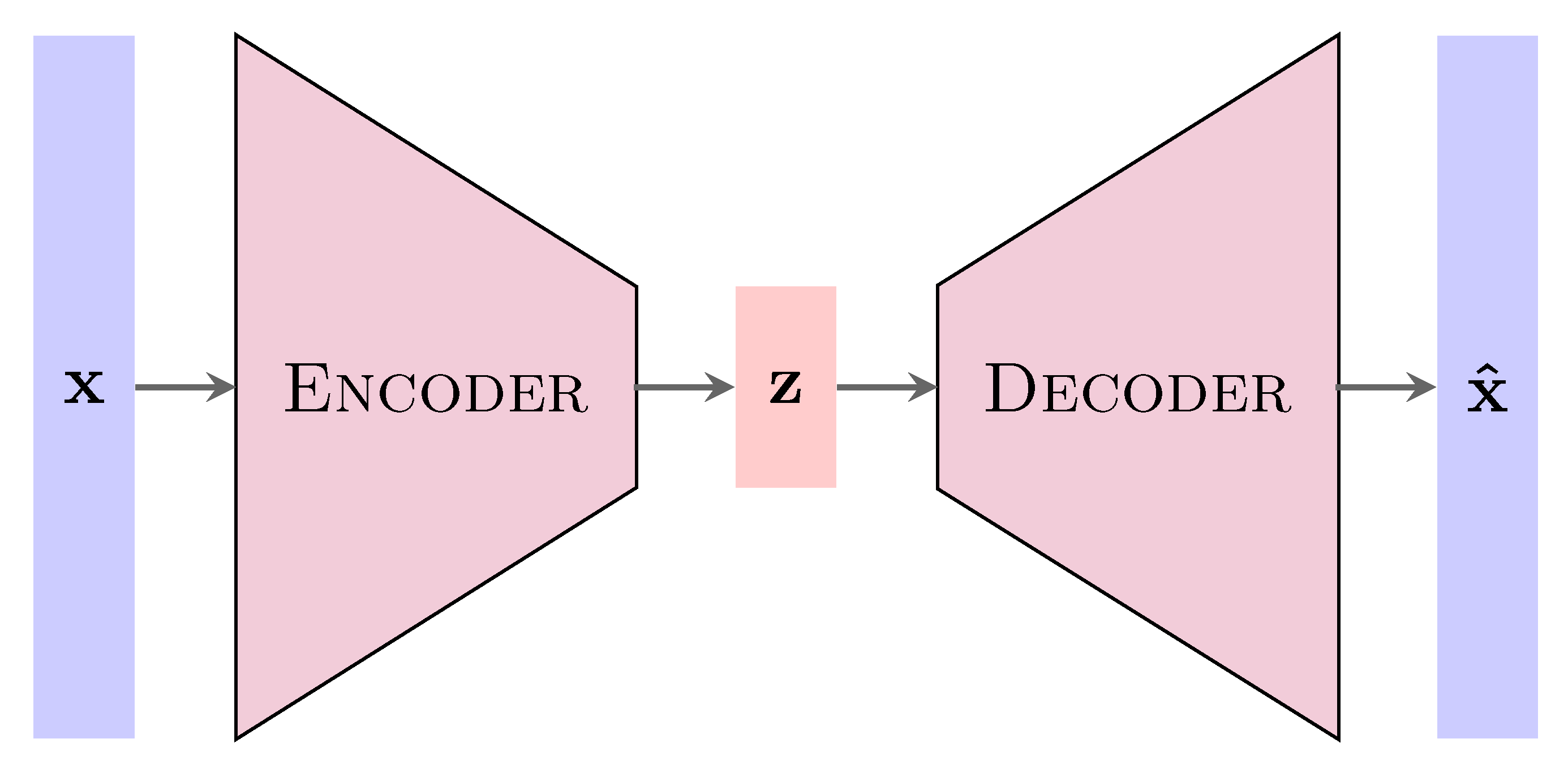
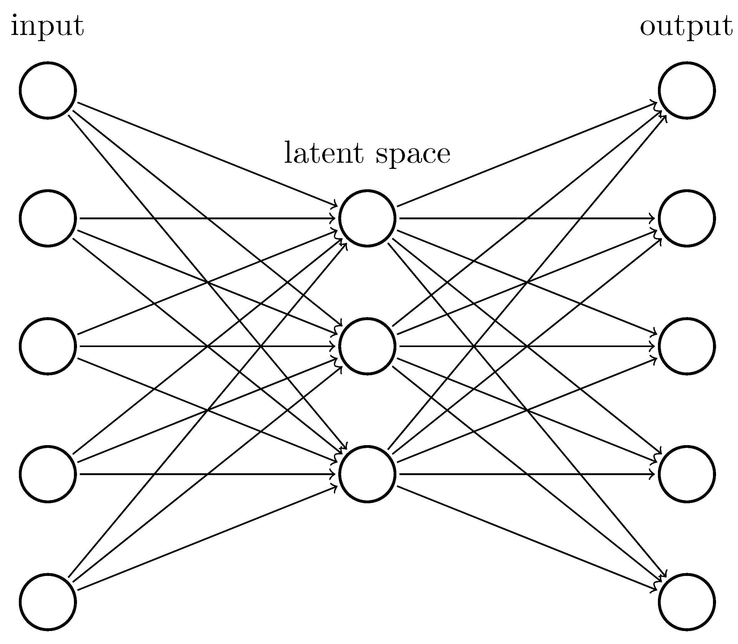
2.2.5. Autoencoder Neural Networks

As for the task of anomaly detection, we adopted AEs, which are the algorithms best-suited for our needs [19]. The logic of such DL methods lies in the capacity to suitably reconstruct the inputs produced by the same process that generates the training instances, poorly reconstructing any instance whose underlying production process differs from the “healthy” process. This is realized by inferring the statistics of reconstruction error from training data, that is the 2 distance between the input and its reconstructed counterpart, then introducing a threshold to distinguish regular from anomalous instances (Figure 5). Anomalous trends can also be identified by tracking reconstruction errors over time to monitor slow parameter variations that correspond to structural deterioration. In this case, training data are acquired in an entirely healthy state of the structure so that AI is unable to learn how to directly identify possible anomalies embedded in the data.
The input data x are mapped to the lower dimensional vector ( z ) through an artificial neural network (the encoder); then, x ^ is obtained from z through the action of another artificial neural network that is symmetric with respect to the encoder (the decoder). The training phase aims to let the parameters of the network converge to the values that make x ^ similar to x in some suitable metrics. We adopted multilayer perceptrons (MLPs), a powerful universal function approximator, to model the non-linear relationship between the input data ( x ) and the lower dimensional vector ( z ) (encoding) and between the lower dimensional vector ( z ) and x ^ (decoding) [20]. In addition to a preset non-linear activation function, the MLP is defined by weights and biases. With respect to the weights and biases of the encoder MLP and decoder MLP, the training objective is to minimize the loss function between the input data ( x ) and their reconstruction ( x ^ ).
The rows ( x i i = 1 N windows ) of matrix X represent single input instances for the AE. Since we expected any variation to be minor, we opted for the best-performing configuration for the artificial neural networks as determined by a random search procedure [21].
The first algorithm tested was a vanilla AE with input dimension n and one hidden intermediate layer, which represents the latent space and has dimension d = n 1 . The graph is fully connected, as depicted in Figure 6, and a hyperbolic tangent is used as an activation function.
In the training phase, the normalized sum of Euclidean distances between the inputs and outputs was adopted as a loss function. Let f θ , ϕ x i be the reconstructed version of input x i , where θ and ϕ indicate the collection of parameters of the encoding and decoding portions, respectively. For the reconstruction error, we take the following quantity:
e θ , ϕ x i = x i f θ , ϕ x i 2 .
The loss function is obtained by averaging the whole training dataset:
L AE X = 1 N windows i = 1 N windows e θ , ϕ x i ,
so that biases and weights converge to the values that best allow the network to obtain outputs as similar as possible to the inputs belonging to the training set in the 2 norm.
The second neural network adopted in this study was a variational autoencoder (VAE), the architecture of which is described in Figure 7. Unlike the simple vanilla autoencoder, the latent representation is not deterministic, as the latent vector is sampled from a multivariate Gaussian distribution with mean vector μ and diagonal covariance matrix σ 2 I . Let p θ z equal the prior probability of obtaining the latent vector ( z ), p θ z x i equal the posterior distribution of z given x i , and p θ x i z be the conditional probability of x i given z , where θ again represents the collection of encoder parameters. The true posterior distribution is generally intractable and is then approximated by a distribution of ( q ϕ z x i ) ( ϕ the collection of parameters for the decoder), which is chosen to be Gaussian and represents the probability of observing the output ( x i ), given the latent variable ( z ). The evidence lower bound (ELBO) is typically adopted as a loss function for VAEs, which is a mixture of cross entropy between the original and reconstructed dataset and Kullback–Leibler divergence that measures the functional distance between the true prior and the approximated posterior (see [22] for derivation):
L θ , ϕ VAE X = 1 N windows i = 1 N windows θ , ϕ x i ,
θ , ϕ x i = E q ϕ z x i log p θ x i z KL q ϕ z x i p θ z .
The first term on the right-hand side of (6) can be estimated through a reparameterization trick, while Kullback–Leibler divergence assumes a simple expression after forcing p θ z to be a standard Gaussian on R d , where d is the size of the hidden space. For details, we again recommend consulting [22].
For the sake of notational simplicity, hereafter, we use e i e θ , ϕ x i .

2.2.6. Statistics of the Reconstruction Error

From a probabilistic point of view, we assume that the sequence of reconstruction errors ( e i i = 1 N windows ) represents a collection of independent, identically distributed random variables on R + . This is strictly true in the case of our simulated dataset, since train runs are mutually independent by construction. Nevertheless, when considering real data, features extracted from any two time windows are not independent a priori. However, we assume that conditions are matched once environmental effects have been compensated through differentiation, seasonality, and trend removal.
According to this hypothesis, the resulting reconstruction error statistics are a generalized chi-square distribution because components of x i and its reconstructed counterpart are, in principle, correlated. Various methods can be applied to deduce probability distribution ( p e i ) from data, thereby establishing a threshold to distinguish undamaged from damaged data in the inference phase. Once threshold α 0 , 1 is established, a given instance can be considered anomalous when its reconstruction error (e) is such that p e < α . We used the kernel density estimation (KDE) method to infer the probability density function (pdf) of the underlying process. In our application, the bandwidth (h) of the kernel, which is the main parameter of the method, was estimated via Silverman’s rule of thumb ( h = 0.9 min σ e , IQR 1.34 N windows 1 5 ), where σ e is the standard deviation of reconstruction errors, and IQR represents the interquartile range. The threshold for acceptability ( α ) was fixed at 0.005 , a value that finds its validity a posteriori. Note that in this initial phase of the construction of our approach, we expect a structure in a healthy state to produce false alarms with probability α . To further perfect the approach, a method for alarm validations is required and will be introduced in the future.

3. Results

In the following subsections, we show the results obtained when training and testing our approach on the simulated railway bridge data and on the data acquired from the tower.

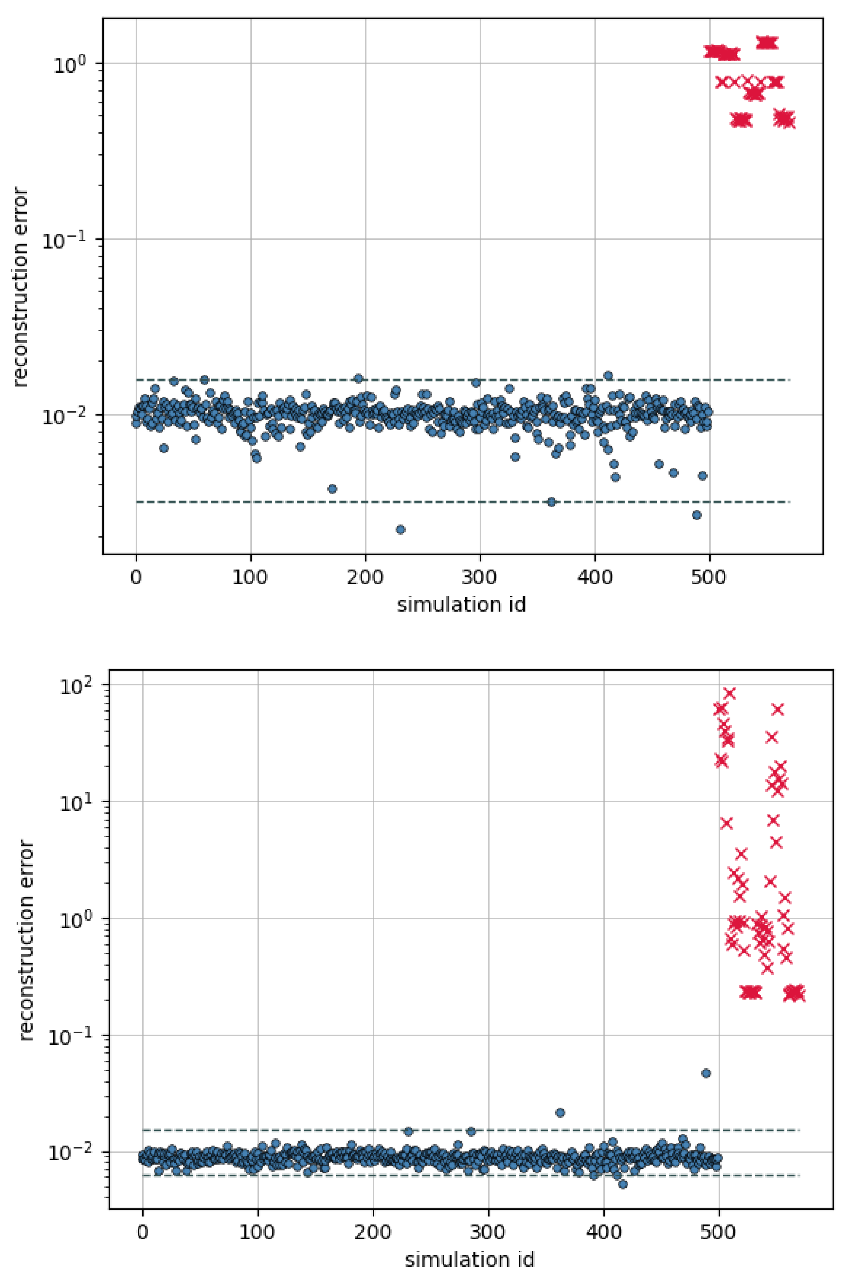
3.1. Results for the Railway Bridge Model

The two algorithms were trained using N windows = 500 train passages, consequently inferring the reconstruction error pdf and obtaining values for e min and e max such that p e < e min < α and p e > e max > α . Figure 8 shows the shape of the pdfs deduced from the training data for AE and VAE, alongside the corresponding frequency histogram.
We initially focused on the predictive capability of the two algorithms as anomaly detectors by introducing damage on node DC 1 . Specifically, FEM dynamics were run after the elastic modulus of the mentioned beam element was reduced by factors of 0.01, 0.02, 0.03, 0.04, 0.05, 0.06, and 0.10, considering 10 time windows for each of these percentages of damage. In addition, we ran 25 further simulations for the undamaged bridge in order to check if the trained algorithms would classify the corresponding inputs as non-anomalous. Figure 9 shows the collection of reconstruction errors for the training set (from 0 to 499, blue) and for the test set corresponding to the 25 undamaged datasets (500 to 524, green regular and red if anomalous) using thresholds (dashed gray lines) corresponding to the values of e min and e max . For the AE, the mean reconstruction error of the training set is μ training AE 1.00 × 10 2 , compared with a value of μ test AE , undamaged 9.53 × 10 3 for the set of the 10 undamaged tests. For the VAE, we obtained μ training VAE 8.90 × 10 3 and μ test VAE , undamaged 8.55 × 10 3 . Both the average reconstruction error values calculated for the test sets are statistically compatible (regarding the statistics deduced from training data) with the means of the training sets (significant within 1 σ ).
Figure 10 shows the collection of reconstruction errors for the training set and the aforementioned damage configurations (enumerated from 500 to 559 (red) in increasing damage order), adopting the log scale for the y-axis, since reconstruction errors spread on various scales. Notice that both algorithms recognize all the "damaged" instances as anomalous, although the reconstruction error appears to be non-monotone in the elastic modulus reduction. It is also worth noting that the VAE is, in this case, more damage-sensitive compared to the AE-based solution, since the errors corresponding to the test set cover a larger interval. This is also a consequence of the VAE’s pdf appearing more peaked around its maximum. The computational costs are comparable for the two neural network autoencoders employed in this simulation.
We performed a second test running numerical dynamics simulations for each of the 32 damage locations as shown in Figure 2. In order to ensure strong data consistency, we fixed the mass and the velocity of the train crossing the bridge to the mean values of 62 tons and 8.33 m/s, respectively, and reduced the elastic moduli of beam elements by a factor of 0.02. Figure 11 again illustrates the reconstruction errors for the training sets and for the 32 different damage scenarios. The evidence supports the conclusion that our solutions correctly classify all the instances provided as inputs as anomalous.

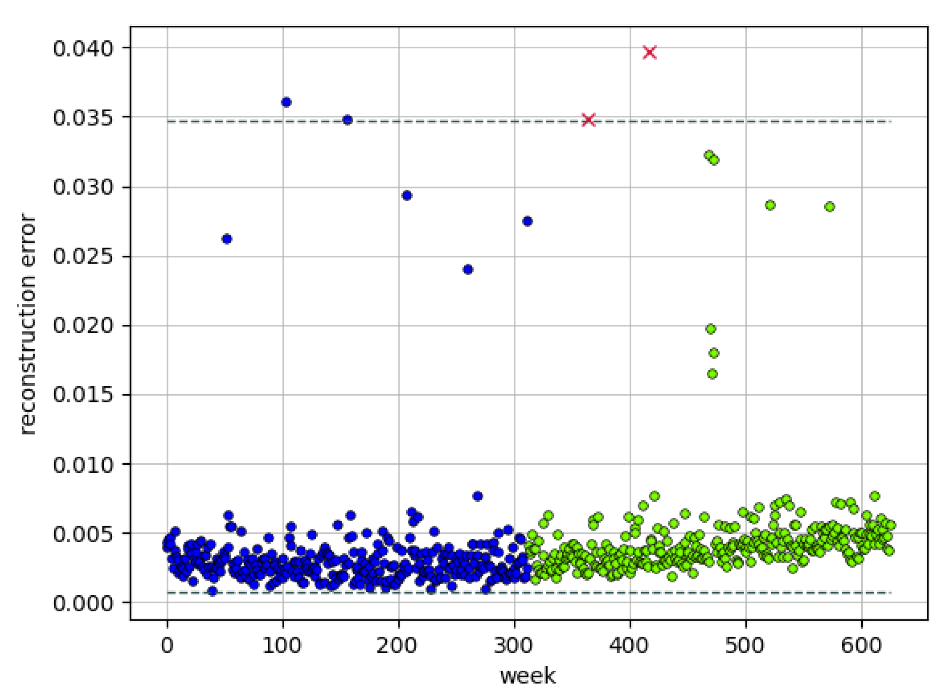
3.2. Results for the Tower Data

The purpose of this case study is to establish whether or not the tower exhibits anomalous trends in the period of time during which it was monitored, i.e., whether the “inclination rate” is constant over time. Accordingly, we split the dataset into training and test sets, considering data acquired in the first six years of monitoring as training data and data acquired in remaining time history (also consisting of six years) as test data.
Figure 12 and Figure 13 show temperature and inclinometer time series, where time is measured in hours starting from midnight on 1 January 2009. It is apparent that I x and I y follow temperature seasonality, although such data seem to exhibit an overall negative trend.
Table 3 reports the values of the angular coefficients obtained for the training and the test sets after data standardization and fitting. Such values make it evident that a change in trends occurs when passing from the training to test sets, particularly affecting the two inclination time series whose rate is one order of magnitude above the change rate of temperature. In fact, the registered temperature appears to be more stable during the monitored years. It is also worth noticing that I y varies more abruptly when compared with the change affecting inclination ( I x ).
Figure 14 and Figure 15 show the reconstruction errors for the training and test phases of both AE and VAE artificial neural networks, with the points sorted in increasing temporal order. Although nearly all the test set reconstruction errors lie in the confidence region, there is an increasing trend for the zone. This is corroborated by linear interpolation of error data. Regarding the AE, we obtained angular coefficients of 2.17 × 10 6 and 4.44 × 10 6 for the training and test set, respectively, while for VAE, we obtained angular coefficients of 2.78 × 10 6 and 3.99 × 10 6 . This can be interpreted as a small trend change in the data, although we do not have any further information (e.g., regarding soil movements) to attribute this to some specific reason.

3.3. Comparison Results

In order to compare our strategy with other popular methods commonly employed in unsupervised cases of anomaly detection in streaming data [23,24], we modified our framework slightly to perform the classification task using isolation forests (IFs) [25] and the Density-Based Spatial Clustering of Applications with Noise (DBSCAN) [26] algorithm.
In this experimental setup, preprocessing was left unchanged from the previously described flow, as the only adjustment regards the AI technique used for anomaly detection. Only the simulated railway bridge data were used, for which the labels are known a priori, and, for each time window, features were extracted, concatenated, and subjected to PCA projection, retaining the same amount of information as before in order to start with the same training and test set used for the AE and VAE. Although both freshly introduced algorithms performed well on synthetic data, here, we discuss the reasons why a deep neural network strategy is still considered preferential for general purposes.
IFs are a sort of unsupervised version of random forests (RFs), and their task consists of constructing binary decision trees to isolate instances in the training dataset in such a way that regular data require many more splits with respect to anomalies to be unambiguously identified. Namely, regular instances are reached by tracing a long path from the root to the corresponding leaf, while outliers need short paths to be reached. Since average paths are logarithmic in the number of instances used to train a single tree, an exponential score is associated with each data point (x):
s x , m = 2 h x c m ,
where m is the total number of instances, h x represents the path length for x, · denotes averages across the whole forest of trees, and c m is a normalization constant that, for any, m > 2 is given by:
c m = 2 H m 1 2 m 1 / m ,
where H m is the harmonic number. Notice that s 0 , 1 , and typically, if s is close to 1, the corresponding instance is very likely to be anomalous, while if s is less than 0.5, s is likely to be a regular instance. The algorithm takes two hyperparameters as inputs, i.e., the number of trees (t) forming the forest and the size ( ψ ) of each subset extracted from the original dataset. Following empirical indications provided in [25], we set t = 100 and ψ = 2 8 .
For our test, we used the IsolationForest module contained in the scikit-learn Python library. After preprocessing, the sequence of steps defining our version of the method are as follows:
-
The algorithm is trained using the n = 500 available instances;
-
A score is obtained for each instance belonging to the training set in order to construct a prevision method in a way similar to that defined previously, although the underlying pdf is different from that describing the autoencoder’s reconstruction errors;
-
A threshold of α = 0.005 is fixed to reject test instances (x) with a probability that is estimated to be less than α to be observed.
With reference to Figure 16a–c, it is clear that IF correctly classifies the 25 non-anomalous test instances (the scores fall within the two thresholds) and all damaged scenarios. Figure 16b refers to the sets in which damages span from 1 to 10 percent for the element labeled as DC 1 , while Figure 16c shows the scores corresponding to the test simulations in which each element has been damaged by reducing the elastic moduli by a factor of 0.02.
DBSCAN is also one of the most popular algorithms for anomaly detection in a non-supervised context; it is a clustering method based on density criteria. It takes two main parameters as input: a distance ( ε ) and an integer (M), which is the minimum number of points that a cluster must contain. The algorithm divides data in two or more clusters depending on the mutual distance of points, with the exception of data that remain isolated, which are then considered as anomalies. Although DBSCAN is widely employed for unsupervised outlier isolation, the choice of hyperparameters ( ε and M) is crucial to obtain suitable results, although empirical evidence for selection of suitable combinations has been reported [26]. Moreover, for datasets whose points lie in a high-dimensional space, even the choice of appropriate metrics represents a relevant issue [26]. Nevertheless, in order to mimic a training-test mechanism, we adapted DBSCAN to our strategy as described below:
-
At fixed M, find ε M as the unique value such that for any ε < ε M , the algorithm detects one or more anomalies in the training set, and for any ε ε M , no anomalies are identified.
-
For any instance in the test set:
-
Add the new instance to the training set;
-
Launch the DBSCAN algorithm with parameters M and ε M and check if the new instance is labeled as an anomaly.
The reason why test instances are added to the training set one at a time and training and test sets are not directly merged lies in the fact that a single instance slightly perturbs the cluster constructions. Regarding the choice of M, it is generally recommended to choose values such that M d + 1 , with d as the dimension in which instances lie. Since our dataset is small if compared to the number of projected features, we considered M = 100 as a suitable compromise for this specific case. As for the previously adopted algorithm, DBSCAN correctly classified all the proposed test instances.
Table 4 shows the results obtained by the different classification algorithms.
In our tests, all the algorithms employed for the classification task performed well for both regular and anomalous time windows. This is also due to the fact that the preprocessing steps are actually capable of extracting a fair amount of information that characterizes most of the signal properties from raw time series. Nevertheless, we believe that the neural network approach is best-suited for the purpose of SHM, as, although the other methods used in this case do what is needed, they could suffer from critical issues when adopted on a large scale. IFs may actually be adapted to deal with large datasets by generating sufficiently large forests of trees (since ψ should remain small to prevent swamping effects), but their structure appears to be far less flexible if compared with our proposed neural-network-based solution. More precisely, network layers can be suitably chosen among several solutions depending on the underlying traits of the dataset; for example, temporal dependencies can be managed by substituting simple layers with LSTM layers, and overfitting can be prevented by employing convolutional layers. In this sense, IFs are less adaptable to the widest range of scenarios. However, this method is advantageous in that its computational costs are linear in the training set dimension, and it induces a very natural statistic for the path lengths. Conversely, DBSCAN appears to be very slow compared to other methods because it requires a new training stage whenever new data must be checked.

4. Discussion

The results obtained so far with simulated data appear promising for the possible future establishment of a well-posed strategy for anomaly detection in the context of SHM. There are positive indicators that confirm the reliability of our proposed approach at a theoretical level, in addition to the improvements made by managing the whole complex sequence of data manipulations through a unique, well-integrated software that uses the HDF5 format for all I/O operations. Although the simulated data refer to an ideal scenario and no external sources of noise affected data at an environmental or hardware level, both trained AI algorithms were capable of distinguishing between damaged and undamaged cases and labeling even minimally damaged configurations as anomalous. This strongly indicates that, even without further refinements of preprocessing techniques and more appropriate hyperparameter settings, this early version of our anomaly detection approach may work appropriately. Encouraging indications also come from the analysis of real thermometric and inclinometer data collected by the network of sensors installed on the tower in Ravenna. Even if the underlying process that regulates the tower is not stationary, as reflected in data that exhibit a visible trend of inclinations ( I x and I y ), AI was still capable of capturing a small change in the inclinometer trend when passing from the training set to the test data, provided stationarization was performed before preprocessing.

5. Conclusions

In this work, we proposed a simple yet reliable integrated approach for SHM in a full data-driven case. The proposed approach consisted of different phases from data acquisition to feature extraction, preprocessing, reduction, and anomaly detection using artificial neural network AEs. Tests were conducted on simulated data, as well as data acquired from physical sensors positioned on a structure, specifically the Historical Tower of Ravenna (Italy). The obtained results in terms of reconstruction error are very promising. The proposed method was also compared to other state-of-the-art anomaly detection methods, as our approach is able to recognize healthy states and classify the various configurations of damage types/severity as anomalous with very high success rates. Nevertheless, the proposed approach deserves more investigations, as we were unable to define a connection between elastic modulus reduction and the obtained output.
Future work will focus on refining the process of feature selection and exploring the space of the artificial neural network’s hyperparameters to enable our solution to estimate the actual damage level based on the value of the obtained reconstruction error. In addition to dimensionality reduction, we will investigate on the application of feature stacking on our data as in [27,28]. We will also integrate supervised algorithms in an attempt to identify possible damage locations from test data. The introduction of a digital twin of the monitored structure would also improve the overall accuracy of the solution in order to double check the results obtained by the data-driven algorithm to reduce false alarms in the damage detection process.

Author Contributions

Conceptualization, R.B., M.B., M.P., A.A. and G.C.; methodology, R.B., M.B., M.P., A.A. and G.C.; software, R.B., M.B. and M.P.; validation, R.B., M.B. and M.P.; formal analysis, R.B., M.B., M.P., A.A. and G.C.; investigation, R.B., M.B., M.P., A.A. and G.C.; resources, R.B., M.B., M.P. and G.C.; data curation, R.B., M.B. and M.P.; writing—original draft preparation, R.B., M.B., M.P., A.A. and G.C.; writing—review and editing, R.B., M.B., M.P., A.A. and G.C.; visualization, R.B., M.B., M.P., A.A. and G.C.; supervision, R.B., M.B., M.P., A.A. and G.C. All authors have read and agreed to the published version of the manuscript.

Funding

The study presented in this article was partially funded by the Project GENESIS: seismic risk manaGEmeNt for the touristic valorisation of thE hiStorIcal centers of Southern italy. PON MIUR “Research and Innovation” 2014–2020 and FSC. D.D. 13 July 2017 n. 1735. Industrial research and experimental development projects in the 12 Smart Specialization areas. Specialization area: Cultural Heritage. Project Code ARS01_00883. The opinions and conclusions presented by the authors do not necessarily reflect those of the funding agency.

Data Availability Statement

The data presented in this study are available upon request from the corresponding author.

Conflicts of Interest

The authors declare no conflict of interest.

References

  1. Hoshyarmanesh, H.; Abbasi, A.; Moein, P.; Ghodsi, M.; Zareinia, K. Design and implementation of an accurate, portable, and time-efficient impedance-based transceiver for structural health monitoring. IEEE/ASME Trans. Mechatron. 2017, 22, 2089–2814. [Google Scholar] [CrossRef]
  2. Sohn, H.; Farrar, C.R.; Hemez, F.M.; Czamecki, J.J. A Review of Structural Health Review of Structural Health Monitoring Literature 1996–2001. In Proceedings of the Third World Conference on Structural Control, Como, Italy, 7–12 April 2002. [Google Scholar]
  3. Rytter, A. Vibrational Based Inspection of Civil Engineering Structures. Ph.D. Thesis, Aalborg University, Aalborg, Denmark, 1993. [Google Scholar]
  4. Farrar, C.R.; Worden, K. Structural Health Monitoring: A Machine Learning Perspective; Wiley: Oxford, UK, 2013. [Google Scholar]
  5. Tibaduiza Burgos, D.A.; Gomez Vargas, R.C.; Pedraza, C.; Agis, D.; Pozo, F. Damage identification in structural health monitoring: A brief review from its implementation to the use of data-driven applications. Sensors 2020, 20, 733. [Google Scholar] [CrossRef] [PubMed]
  6. Nick, W.; Shelton, J.; Asamene, K.; Esterline, A.C. A Study of Supervised Machine Learning Techniques for Structural Health Monitoring. MAICS 2015, 1353, 36. [Google Scholar]
  7. Giglioli, V.; Venanzi, V.; Poggioni, I.; Milani, A.; Ubertini, F. Autoencoders for unsupervised real-time bridge health assessment. Comput. Civ. Infrastruct. Eng. 2023, 38, 959–974. [Google Scholar] [CrossRef]
  8. Ma, X.; Lin, Y.; Nie, Z.; Ma, H. Structural damage identification based on unsupervised feature-extraction via Variational Auto-encoder. Measurement 2020, 160, 107811. [Google Scholar] [CrossRef]
  9. Pollastro, A.; Testa, G.; Bilotta, A.; Prevete, R. Unsupervised detection of structural damage using Variational Autoencoder and a One-Class Support Vector Machine. arXiv 2022, arXiv:2210.05674. [Google Scholar]
  10. Cauteruccio, F.; Fortino, G.; Guerrieri, A.; Terracina, G. Discovery of Hidden Correlations between Heterogeneous Wireless Sensor Data Streams. In Internet and Distributed Computing Systems, Proceedings of the 7th International Conference, IDCS 2014, Calabria, Italy, 22–24 September 2014; Springer International Publishing: Cham, Switzerland, 2014; pp. 383–395. [Google Scholar] [CrossRef]
  11. Cauteruccio, F.; Fortino, G.; Guerrieri, A.; Liotta, A.; Mocanu, D.C.; Perra, C.; Terracina, G.; Torres Vega, M. Short-long term anomaly detection in wireless sensor networks based on machine learning and multi-parameterized edit distance. Inf. Fusion 2019, 52, 13–30. [Google Scholar] [CrossRef]
  12. Petracca, M.; Candeloro, F.; Camata, G. STKO User Manual; ASDEA Software Technology: Pescara, Italy, 2017. [Google Scholar]
  13. Ubertini, F.; Gentile, C.; Materazzi, A.L. Automated modal identification in operational conditions and its application to bridges. Eng. Struct. 2013, 46, 264–278. [Google Scholar] [CrossRef]
  14. Parisi, F.; Mangini, A.M.; Fanti, M.P.; Adam, J.M. Automated location of steel truss bridge damage using machine learning and raw strain sensor data. Autom. Constr. 2022, 138, 104249. [Google Scholar] [CrossRef]
  15. Ulyah, S.M.; Mardianto, M.F.F. Comparing the Performance of Seasonal ARIMAX Model and Nonparametric Regression Model in Predicting Claim Reserve of Education Insurance. J. Phys. Conf. Ser. 2019, 1397, 012074. [Google Scholar] [CrossRef]
  16. Buckley, T.; Bidisha, G.; Pakrashi, V. A feature extraction & selection benchmark for structural health monitoring. Struct. Health Monit. 2023, 22, 2082–2127. [Google Scholar]
  17. Barandas, M.; Folgado, D.; Fernandes, L.; Santos, S.; Abreu, M.; Bota, P.; Liu, H.; Schultz, T.; Gamboa, H. TSFEL: Time Series Feature Extraction Library. SoftwareX 2020, 11, 100456. [Google Scholar] [CrossRef]
  18. Ringnér, M. What is principal component analysis? Nat. Biotechnol. 2008, 26, 303–304. [Google Scholar] [CrossRef] [PubMed]
  19. Bank, D.; Koenigstein, N.; Giryes, R. Autoencoders. arXiv 2020, arXiv:2003.05991. [Google Scholar]
  20. Jin, F.; Sengupta, A.; Cao, S. mmFall: Fall Detection Using 4-D mmWave Radar and a Hybrid Variational RNN AutoEncoder. IEEE Trans. Autom. Sci. Eng. 2022, 19, 1245–1257. [Google Scholar] [CrossRef]
  21. Bergstra, J.; Bengio, Y. Random Search for Hyper-Parameter Optimization. J. Mach. Learn. Res. 2012, 13, 281–305. [Google Scholar]
  22. Kingma, D.P.; Welling, M. Auto Encoding Variational Bayes. arXiv 2013, arXiv:1312.6114. [Google Scholar]
  23. Ding, Z.; Fei, M. An Anomaly Detection Approach Based on Isolation Forest Algorithm for Streaming Data using Sliding Window. IFAC Proc. Vol. 2013, 46, 12–17. [Google Scholar] [CrossRef]
  24. Emadi, H.S.; Mazinani, S.M. A Novel Anomaly Detection Algorithm Using DBSCAN and SVM in Wireless Sensor Networks. Wirel. Pers. Commun. 2018, 98, 2025–2035. [Google Scholar] [CrossRef]
  25. Liu, F.T.; Ting, K.M.; Zhou, Z.H. Isolation Forest. In Proceedings of the 2008 Eighth IEEE International Conference on Data Mining, Pisa, Italy, 15–19 December 2008; pp. 413–422. [Google Scholar] [CrossRef]
  26. Ester, M.; Kriegel, H.P.; Sander, J.; Xu, X. A Density-Based Algorithm for Discovering Clusters in Large Spatial Databases with Noise. In Proceedings of the Second International Conference on Knowledge Discovery and Data Mining, KDD’96, Portland, OR, USA, 2–4 August 1996; AAAI Press: Washington, DC, USA, 1996; pp. 226–231. [Google Scholar]
  27. Hartmann, Y.; Liu, H.; Schultz, T. Feature Space Reduction for Multimodal Human Activity Recognition. In Proceedings of the 13th International Joint Conference on Biomedical Engineering Systems and Technologies, BIOSTEC 2020, Valletta, Malta, 24–26 February 2020; SCITEPRESS: Setúbal, Portugal, 2020; pp. 135–140. [Google Scholar] [CrossRef]
  28. Hui, L. Biosignal Processing and Activity Modeling for Multimodal Human Activity Recognition. Ph.D. Thesis, Universität Bremen, Bremen, Germany, 2021. [Google Scholar] [CrossRef]
Figure 1. Schematic representation of the bridge and sensor positions.
Bdcc 07 00099 g001
Figure 2. Locations of the 32 elements whose elastic modulus the user can reduce. Legend: DC, diagonal in compression; DT, diagonal in tension; CC, chord in compression; CT, chord in tension.
Bdcc 07 00099 g002
Figure 3. Flow chart of the comprehensive process described in the text, from data acquisition to decision making.
Bdcc 07 00099 g003
Figure 4. Values of m i for the 50 least correlated features.
Bdcc 07 00099 g004
Figure 5. Schematic representation of an AE.
Bdcc 07 00099 g005
Figure 6. Schematic representation of the vanilla autoencoder used in this study.
Bdcc 07 00099 g006
Figure 7. Schematic representation of the variational autoencoder used in this study.
Bdcc 07 00099 g007
Figure 8. The pdf (orange lines) inferred from training data in the case of AE (upper) and VAE (bottom). Histograms (blue) were obtained using 20 bins.
Bdcc 07 00099 g008
Figure 9. The reconstruction error for training and non-damaged test sets for AE (top) and VAE (bottom) for the case study of the railway bridge model.
Bdcc 07 00099 g009
Figure 10. The reconstruction error for training and damaged test sets as indicated in the text for AE (top) and VAE (bottom) for the case study of the railway bridge model.
Bdcc 07 00099 g010
Figure 11. The reconstruction error for training and the second damaged test sets as indicated in the text for AE (top) and VAE (bottom) for the case study of the railway bridge model.
Bdcc 07 00099 g011
Figure 12. Temperature data as registered by sensors. T 1 is indicated in blue, T 2 is indicated in green, and T 3 is indicated in orange.
Bdcc 07 00099 g012
Figure 13. Inclinations as registered by sensors. I x is indicated in blue, while I y is indicated in orange.
Bdcc 07 00099 g013
Figure 14. Reconstruction errors for AE.
Bdcc 07 00099 g014
Figure 15. Reconstruction errors for VAE.
Bdcc 07 00099 g015
Figure 16. The scores, as defined in the text, corresponding to the training and the test sets for the IF. Blue points represent training set scores, green points are scores that fall within the confidence region, and red crosses are anomalies. The same three scenarios investigated using AEs are represented: no damage at all (a), constantly decreased elastic modulus of D C 1 (b), and damage at 2% for each of the 32 considered beam elements (c).
Bdcc 07 00099 g016
Table 1. List of the features computed by the TSFEL library divided into statistical, temporal, and spectral categories.
StatisticalTemporalSpectral
ECDFAbsolute energyFFT mean coefficients
ECDF percentileArea under the curveFundamental frequency
ECDF percentile countAutocorrelationMFCC
ECDF slopeCentroidLPCC
HistogramEntropyMax power spectrum
Interquantile rangeMean absolute differenceMaximum frequency
KurtosisMean differenceMedian frequency
MaxMedian absolute differencePower bandwidth
MeanMedian differenceSpectral centroid
Mean absolute deviationNegative turning pointsSpectral decrease
MedianPeak-to-peak distanceSpectral distance
Median absolute deviationPositive turning pointsSpectral entropy
MinSignal distanceSpectral kurtosis
Root mean squareSlopeSpectral positive turning points
SkewnessSum absolute differenceSpectral roll-off
Standard deviationTotal energySpectral roll-on
VarianceZero crossing rateSpectral skewness
Neighborhood peaksSpectral slope
Spectral spread
Spectral variation
Wavelet absolute mean
Wavelet energy
Wavelet standard deviation
Wavelet entropy
Wavelet variance
Table 2. List of the 20 least correlated features as defined in the text. The number (n) in the features corresponds to their nth coefficient.
FeatureSensor m i
Wavelet variance 6 A 1 x 0.117
FFT mean coefficient 4 A 1 y 0.119
ECDF 4 A 1 y 0.119
FFT mean coefficient 8 A 1 y 0.119
FFT mean coefficient 5 A 1 y 0.123
FFT mean coefficient 11 A 1 y 0.125
Wavelet variance 7 A 1 x 0.127
Zero crossing rate A 1 x 0.127
ECDF 7 A 1 y 0.128
FFT mean coefficient 7 A 1 y 0.129
FFT mean coefficient 12 A 1 y 0.132
Entropy A 1 y 0.133
ECDF 9 A 1 y 0.134
FFT mean coefficient 1 A 1 y 0.135
ECDF 3 A 1 y 0.137
Autocorrelation A 1 y 0.137
ECDF 6 A 1 y 0.141
ECDF Percentile 1 A 1 y 0.145
ECDF 1 A 1 y 0.149
ECDF 4 A 1 y 0.150
Table 3. Angular coefficients for the linear fits of standardized datasets for the training and test sets.
Angular Coefficient (2009–2015)Angular Coefficient (2016–2021)
T 1 4.09 × 10 6 1.66 × 10 6
T 2 6.71 × 10 6 2.17 × 10 6
T 3 4.79 × 10 6 2.03 × 10 6
I x 1.84 × 10 5 2.25 × 10 5
I y 2.06 × 10 5 3.24 × 10 5
Table 4. Success percentage in the anomaly detection task for the considered algorithms.
Regular DataAnomalous Data
AE96%100%
VAE96%100%
IF100%100%
DBSCAN100%100%
Disclaimer/Publisher’s Note: The statements, opinions and data contained in all publications are solely those of the individual author(s) and contributor(s) and not of MDPI and/or the editor(s). MDPI and/or the editor(s) disclaim responsibility for any injury to people or property resulting from any ideas, methods, instructions or products referred to in the content.

