1. Introduction
Sales forecasts at the SKU (stock-keeping unit) level are essential for effective inventory management, production planning, pricing and promotional strategies, and sales performance tracking [
1]. SKUs represent individual products or product variants within a larger product line. By forecasting sales at the SKU level, businesses can optimize their inventory levels to ensure they have enough stock on hand to meet demand without overstocking and tying up capital. This helps to reduce inventory holding costs and avoid stockouts, which can result in lost sales and dissatisfied customers [
2]. SKU-level sales forecasts can also help businesses plan their production schedules and ensure they have enough raw materials and resources to meet demand. This can help reduce production downtime and minimize waste and inefficiencies. SKU-level sales forecasts can help businesses determine the optimal pricing and promotional strategies for each SKU. For example, if a particular SKU is expected to have high demand, a business may choose to increase the price to maximize profit margins. Alternatively, if a SKU is not selling as well as expected, a business may choose to offer discounts or promotions to stimulate sales. SKU-level sales forecasts also allow businesses to track the performance of individual products and identify trends and patterns in consumer behaviour. This can help businesses make data-driven decisions and adjust their strategies accordingly [
3].
Retailers typically offer a vast range of products, from perishable items such as fresh produce to non-perishable goods such as electronics and clothing. Each product has distinct demand patterns that may differ based on location, time, day of the week, season, and promotional events. Forecasting sales for each of these items can be a daunting and complicated task, particularly since retailers often sell products through multiple channels, including physical stores, online platforms, mobile apps, and marketplaces, each with its own set of difficulties and opportunities that must be considered when forecasting sales. Additionally, in the retail sector, demand forecasting is a regular occurrence, often performed weekly or daily, to ensure optimal inventory levels. As a result, advanced models and techniques are necessary to tackle the forecasting problem, which must be automated to reduce manual intervention, robust to handle various data types and scenarios, and scalable to accommodate large data volumes and changing business requirements [
4].
1.1. Local versus Global Forecasting Models
For decades, the prevailing approach in time-series forecasting has been to view each time series as a standalone dataset [
5,
6]. This has led to the use of localized forecasting techniques that treat each series individually and make predictions based solely on the statistical patterns observed in that series. The Exponential Smoothing State Space Model (ETS) [
7] and Auto-Regressive Integrated Moving Average Model (ARIMA) [
8] are notable examples of such methods. While these approaches have been widely used and have produced useful results in many cases, they have their limitations [
9]. Currently, businesses often collect vast amounts of time-series data from similar sources on a regular basis. For example, retailers may collect data on the sales of thousands of different products, manufacturers may collect data on machine measurements for predictive maintenance, and utility companies may gather data on smart-meter readings across many households. While traditional local forecasting techniques can still be used to make predictions in these situations, they may not be able to fully exploit the potential for learning patterns across multiple time series. This has led to a paradigm shift in forecasting, where instead of treating each individual time series separately, a set of series is seen as a dataset [
10].
A global forecasting model (GFM) has the same set of parameters, such as weights in the case of a neural network [
11], for all the time series (all time series in the dataset are forecast using the same function), in contrast to a local model, which has a unique set of parameters for each individual series. This means that the global model takes into account the interdependencies between the variables across the entire dataset, whereas local models focus only on the statistical properties of each individual series. In the retail industry, it is possible to capture cross-product and cross-region dependencies, which can result in more-accurate forecasts across the entire range of products. When we talk about cross-product dependencies, we are referring to the connection between different products. Alterations in one product can have an impact on the demand or performance of another product. For instance, if two products are complementary or substitutable, changes in the sales of one product can affect the sales of the other. Conversely, the demand for a particular product may exhibit a similar pattern for all varieties, brands, or packaging options in various stores. Cross-region dependencies refer to the link between different regions or locations. Changes in one region, such as fluctuations in economic conditions or weather patterns, may have an effect on the demand or performance in another region. Global forecasting models, typically built using advanced machine learning techniques such as deep learning and artificial neural networks, are gaining popularity, as seen in the works of [
12,
13,
14,
15], and have outperformed local models in various prestigious forecasting competitions such as the M4 [
16,
17] and the recent M5 [
18,
19,
20], as well as those held on the Kaggle platform with a forecasting purpose [
21]. In summary, the recent paradigm shift in forecasting recognizes that analysing multiple time series together as a dataset can yield significant improvements in accuracy and provide valuable insights into underlying patterns and trends. This shift has opened up new opportunities for businesses to leverage machine learning and other advanced techniques to gain a competitive advantage in forecasting and decision making. However, there are still many challenges to overcome, such as the need for skilled data scientists, significant amounts of data and time for training the models, and sufficient computational and data infrastructures. Additionally, to promote the adoption and sustained usage of GFMs in practice, it is essential to have expertise within the organization, along with model transparency and intelligibility, which are crucial attributes for establishing user trust.
1.2. Relatedness between Time Series
The successful aforementioned studies are based on the assumption that GFMs are effective because there exists a relationship between the series (all come hypothetically from similar data-generating processes), enabling the model to recognize complex patterns shared across them. Nevertheless, none of these studies endeavours to elucidate or establish the characteristics of this relationship. Some research has connected high levels of relatedness between series with greater similarity in their shapes or patterns and stronger cross-correlation [
22,
23], while other studies have suggested that higher relatedness corresponds to greater similarity in the extracted features of the series being examined [
24].
Montero-Manso and Hyndman’s recent work [
9] is the first to provide insights into this area. Their research demonstrates that it is always possible to find a GFM capable of performing just as well or even better than a set of local statistical benchmarks for any dataset, regardless of its heterogeneity. This implies that GFMs are not inherently more restricted than local models and can perform well even if the series are unrelated. Due to the utilization of more data, global models can be more complex than local ones (without suffering from overfitting) while still achieving better generalization. Montero-Manso and Hyndman suggest that the complexity of global models can be achieved by increasing the memory/order of autoregression, using non-linear/non-parametric methods, and employing data partitioning. The authors provide empirical evidence of their findings through the use of real-world datasets.
Hewamalage et al. [
25] aimed to investigate the factors that influence GFM performance by simulating various datasets with controlled characteristics, including the homogeneity/heterogeneity of series, pattern complexity, forecasting model complexity, and series number/length. Their results reveal that relatedness has a strong connection with other factors, including data availability, data complexity, and the complexity of the forecasting approach adopted, when it comes to GFM performance. Furthermore, in challenging forecasting situations, such as those involving short or heterogeneous series and limited prior knowledge of data patterns, GFMs’ complex non-linear modelling capabilities make them a competitive option.
Rajapaksha et al. [
26] recently introduced a novel local model-agnostic interpretability approach to address the lack of interpretability in GFMs. The approach employs statistical forecasting techniques to explain the global model forecast of a specific time series using interpretable components such as trend, seasonality, coefficients, and other model attributes. This is achieved by defining a locally defined neighbourhood, which can be done through either bootstrapping or model fitting. The authors conducted experiments on various benchmark datasets to evaluate the effectiveness of this framework. They evaluated the results both quantitatively and qualitatively and found that the two approaches proposed in the framework provided comprehensible explanations that accurately approximated the global model forecast.
Nevertheless, the major real-world datasets are, by nature, heterogeneous, including series that are clearly unrelated, such as the M4 forecasting competition, whose dataset is a broad mix of unaligned time series across many different domains [
25].
1.3. Model Complexity
Kolmogorov’s theory [
27] explains the concept of complexity, which can be technically described as follows. We begin by establishing a syntax for expressing all computable functions, which could be an enumeration of all Turing machines or a list of syntactically correct programs in a universal programming language such as Java, Lisp, or C. From there, we defined the Kolmogorov complexity of a finite binary string (every object can be coded as a string over a finite alphabet—say, the binary alphabet) as the length of the shortest Turing machine, Java program, etc., in the chosen syntax. Thus, to each finite string is assigned a positive integer as its Kolmogorov complexity through this syntax. Ultimately, the Kolmogorov complexity of a finite string represents the length of its most-compressed version and the amount of information (in the form of bits) contained within it. Although Kolmogorov complexity is generally believed to be theoretically incomputable [
28], recent research by Cilibrasi and Vitanyi [
29] has demonstrated that it can be approximated using the decompressor of modern real-world compression techniques. This approximation involves determining the length of a minimum and efficient description of an object that can be produced by a lossless compressor. As a result, to estimate the complexity of our models in this experiment, we rely on the size of their gzip compressions, which are considered very efficient and are widely used. If the output file of a model can be compressed to a very small size, it suggests that the information contained within it is relatively simple and structured and can be easily described using a small amount of information. This would indicate that the model is relatively simple. Conversely, if the output file of a model is difficult to compress, and requires a large amount of storage space, this suggests that the information contained within it is more complex and is structured in a way that cannot be easily reduced. This indicates that the model is more complex. It is worth noting that this approach to measuring algorithmic complexity of models may depend on the data used, but since all models in our experiment are based on the same data, we do not factor the data into the compression.
The number of parameters in a model can also be a useful heuristic for measuring the model’s complexity [
30]. Each parameter represents a degree of freedom that the model has in order to capture patterns in the data. The more parameters a model has, the more complex its function can be, and the more flexible it is to fit a wide range of training data patterns. Deep learning models differ structurally from traditional machine learning models and have significantly more parameters. These models are consistently over-parametrised, implying that they contain more parameters than the optimal solutions and training samples. Nonetheless, research has demonstrated that extensively over-parametrised neural networks often show strong generalization capabilities. In fact, several studies suggest that larger and more-complex networks generally achieve superior generalization performance [
31].
1.4. Key Contributions
Despite all of the aforementioned efforts, there has been a lack of research on how the relatedness between series impacts the effectiveness of GFMs in real-world demand-forecasting problems, especially when dealing with challenging conditions such as the highly lumpy or intermittent data very common in retail. The research conducted in this study was driven precisely by this motivation: to investigate the cross-learning scenarios driven by the product hierarchy commonly employed in retail planning that enable global models to better capture interdependencies across products and regions. We provide the following contributions that help understand the potential and applicability of global models in real-world scenarios:
Our study investigates possible dataset partitioning scenarios, inspired by the hierarchical aggregation structure of the data, that have the potential to more effectively capture inter-dependencies across regions and products. To achieve this, we utilize a prominent deep learning forecasting model that has demonstrated success in numerous time-series applications due to its ability to extract features from high-dimensional inputs.
We evaluate the heterogeneity of the dataset by examining the similarity of the time-series features that we deem crucial for accurate forecasting. Some features, which are deliberately crafted, prove especially valuable for intermittent data.
In order to gauge the complexity of our models during the experiment, we offer two quantitative indicators: the count of parameters contained within the models and the compressibility of their output files as determined by Kolmogorov complexity.
A comprehensive evaluation of the forecast accuracy achieved by the global models of the various partitioning approaches and local benchmarks using two error measures is presented. These measures are also used to perform tests on the statistical significance of any reported differences.
The empirical results we obtained provide modelling guidelines that are easy for both retailers and software suppliers to implement regarding the trade-off between data availability and data relatedness.
The layout of the remainder of this paper is as follows.
Section 2 describes our forecasting framework developed for the evaluation of the cross-learning approaches, and
Section 3 provides the details about its implementation.
Section 4 presents and discusses the results obtained, and
Section 5 provides some concluding remarks and promising areas for further research.
2. Forecasting Models
Due to the impressive accomplishments of deep learning in computer vision, its implementation has extended to several areas, including natural language processing and robot control, making it a popular choice in the machine learning domain. Despite being a significant application of machine learning, the progress of using deep learning in time-series forecasting has been relatively slower compared to other areas. Moreover, the lack of a well-defined experimental protocol makes its comparison with other forecasting methods difficult. Given that deep learning has demonstrated superior performance compared to other approaches in multiple domains when trained on large datasets, we were confident that it could be effective in the current context. However, few studies have focused on deep learning approaches for intermittent demand [
32]. Forecasting intermittent data involves dealing with sequences that have sporadic values [
33]. This is a complex task, as it entails making predictions based on irregular observations over time and a significant number of zero values. We selected DeepAR, which is an autoregressive recurrent neural network (RNN) model that was introduced by Amazon in 2018 [
23]. DeepAR is a prominent deep learning forecasting model that has demonstrated success in several time-series applications.
2.1. DeepAR Model
Formally, denoting the value of item
i at time
t by
, the goal of DeepAR is to predict the conditional probability
P of future sales
based on past sales
and covariates
, where
and
T are, respectively, the first and last time points of the future
Note that the time index
t is relative, i.e.,
may not correspond to the first time point of the time series. During training,
is available in both time ranges
and
, known respectively as the conditioning range and the prediction range (corresponding to the encoder and decoder in a sequence-to-sequence model), but during inference,
is not available in the prediction range. The network output at time
t can be expressed as
where
h is a function that is implemented by a multi-layer RNN with long short-term memory (LSTM) cells [
34] parameterised by
. The model is autoregressive in the sense that it uses the sales value at the previous time step
as an input, and recurrent in the sense that the previous network output
is fed back as an input at the next time step. During training, given a batch of
N items
and corresponding covariates
, the model parameters are learned by maximizing the log-likelihood of a fixed probability distribution as follows
where
denotes a linear mapping from the function
to the distribution’s parameters, while
l represents the likelihood of the distribution. Since the encoder model is the same as the decoder, DeepAR uses all of time range
to calculate this loss (i.e.,
in Equation (
3)). DeepAR is designed to predict a 1-step forwarded value. To forecast multiple future steps in the inference, the model repeatedly generates forecasts for the next period until the end of the forecast horizon. Initially, the model is fed with past sequences (
), and the forecast of the first period is generated by drawing samples from the trained probability distribution. The forecast of the first period is then used as an input to the model for generating the forecast of the second period, and so on for each subsequent period. As the forecast is based on past samples from the predicted distribution, the model’s output is probabilistic and not deterministic, and it represents a distribution of sampled sequences. This sampling process is advantageous as it generates a probability distribution of forecasts, which can evaluate the accuracy of the forecasts.
To address the issue of zero-inflated distribution in sales demands, we employed the negative log-likelihood of the Tweedie distribution for the loss function. The Tweedie distribution is a family of probability distributions that is characterized by two parameters: the power parameter, denoted as
p, and the dispersion parameter, denoted as
. The probability density function of the Tweedie distribution is defined as:
where
is the mean parameter of the distribution,
is the gamma function, and
p and
are positive parameters. When
, the Tweedie distribution is a compound Poisson–gamma distribution, which is commonly used to model data with a large number of zeros and positive skewness. The dispersion parameter
controls the degree of variability or heterogeneity in the data. When
is small, the data are said to be highly variable or dispersed, while a large value of
indicates low variability or homogeneity in the data.
Our implementation of the DeepAR models used the PyTorch AI framework [
35] with the
DeepAREstimator method from the
GluonTS Python library [
36].
2.2. Benchmarks
Benchmarks are used to evaluate the performance of forecasting models by providing a standard against which the models can be compared [
37]. By using benchmarks, researchers and practitioners can objectively assess the forecasting accuracy of different models and identify which model performs best for a given forecasting task. Comparing the accuracy of a forecasting model against a benchmark provides a baseline measure of its performance and helps to identify the added value of the model. The two most-commonly utilized models for time-series forecasting are Exponential Smoothing and ARIMA (AutoRegressive Integrated Moving Average). These benchmark models are good references for evaluating the forecasting performance of more-complex models. They provide a baseline for comparison and help to identify whether a more-complex model is justified based on its added accuracy on the benchmark. The seasonal naïve method can be very effective at capturing the seasonal pattern of a time series and is also frequently adopted as a benchmark to compare against more complex models.
2.2.1. ARIMA Models
The seasonal ARIMA model, denoted as ARIMA
, can be written as:
where
is the target time series,
m is the seasonal period,
D and
d are the degrees of seasonal and ordinary differencing, respectively,
B is the backward shift operator,
and
are the regular autoregressive and moving average polynomials of orders
p and
q, respectively,
and
are the seasonal autoregressive and moving-average polynomials of orders
P and
Q, respectively,
, where
is the mean of
and
is a white-noise series (i.e., serially uncorrelated with zero mean and constant variance). Stationarity and invertibility conditions imply that the zeros of the polynomials
,
,
, and
must all lie outside of the unit circle. Non-stationary time series can be made stationary by applying transformations such as logarithms to stabilise the variance and by taking proper degrees of differencing to stabilise the mean. After specifying values for
, and
Q, the parameters of the model
can be estimated by maximising the log likelihood. The Akaike’s Information Criteria (AIC), which is based on the log likelihood and on a regularization term (that includes the number of parameters in the model) to compensate for potential overfitting, can be used for determining the values of
, and
Q. To implement the ARIMA models, we used the
AutoARIMA function from the
StatsForecast Python library [
38], which is a mirror of Hyndman’s [
39]
auto.arima function in the
forecast package of the R programming language.
2.2.2. Exponential Smoothing Models
Exponential smoothing models comprise a measurement (or observation) equation and one or several state equations. The measurement equation describes the relationship between the time series and its states or components, i.e., the level, the trend, and the seasonality. The state equations express how the components evolve over time [
7,
40]. The components can interact with themselves in an additive (A) or multiplicative (M) manner; an additive damped trend (A
d) or multiplicative damped trend (M
d) is also possible. For each model, an additive or multiplicative error term can be considered. Each component is updated by the error process, which is the amount of change controlled by the smoothing parameter. For more details, the reader is referred to [
7] and [
41]. The existence of a consistent multiplicative effect on sales led us to use a logarithm transformation and, consequently, to adopt only linear exponential smoothing models.
Table 1 presents the equations for these models in the state-space modelling framework:
is the time-series observation in period
t,
is the local level in period
t,
is the local trend in period
t,
is the local seasonality in period
t, and
m is the seasonal frequency;
, and
are the smoothing parameters, and
is the error term usually assumed to be normally and independently distributed with mean 0 and variance
, i.e.,
. To implement the exponential smoothing models, we used the
AutoETS function from the
StatsForecast Python library [
38], which is a mirror of Hyndman’s [
7]
ets function in the
forecast package of the R programming language.
2.2.3. Seasonal Naïve
The Seasonal Naïve model is a simple time-series forecasting model that assumes the future value of a series will be equal to the last observed value from the same season. It can be formulated as follows:
where
is the forecasted value of the series at time
t,
is the last observed value from the same season (
m periods ago), and
m is the number of periods in a season (e.g., seven for daily data with weekly seasonality).
3. Empirical Setup
In this section, we present experimental scenarios that use hierarchical aggregation structure-based data partitioning to investigate quantitatively how the relatedness between series impacts the effectiveness of GFMs and their complexity.
3.1. Dataset
To ensure the significance of a study’s findings, it is crucial that it can be reproduced and compared with other relevant studies. Therefore, in this study, we used the M5 competition’s well-established and openly accessible dataset, which is widely recognized as a benchmark for the development and evaluation of time-series forecasting models. The M5 dataset is a large time-series set consisting of sales data for Walmart stores in the United States. The dataset was released in 2020 as part of the M5 forecasting competition, which was organized by University of Nicosia and sponsored by Kaggle [
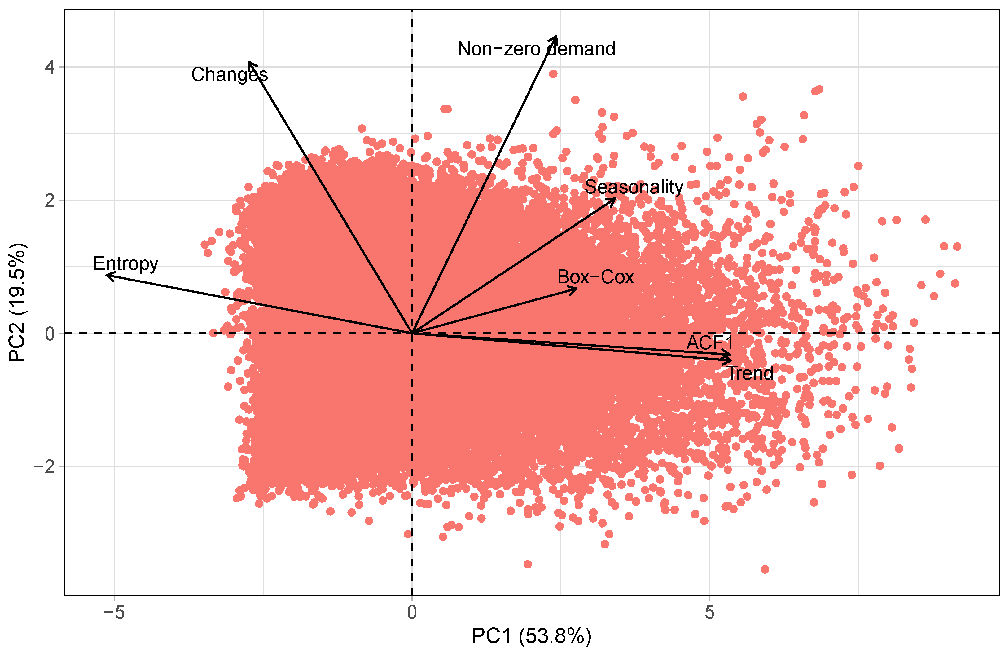
19]. The M5 dataset includes daily sales data for 3049 products and spans a period of 5 years, from 29 January 2011 to 19 June 2016 (1969 days). The dataset is organized hierarchically, with products being grouped into states, stores, categories, and departments. The 3049 products were sold across ten different stores, which were located in three states of the USA: California (CA), Texas (TX), and Wisconsin (WI). California covers four stores (CA1, CA2, CA3, and CA4), while Texas and Wisconsin represent three stores each (TX1, TX2, TX3 and WI1, WI2, WI3). For every store, the products are classified into three main categories: Household, Hobbies, and Foods. These categories are further divided into specific departments. Specifically, the Household and Hobbies categories are each subdivided into two departments (Household1, Household2 and Hobbies1, Hobbies2), while the Foods category is subdivided into three departments (Foods1, Foods2, and Foods3). The main goal of the M5 competition was to develop accurate sales forecasts for the last 28 days from 23 May 2016 to 19 June 2016. The M5 dataset has become a standard reference due to its challenging properties, including high dimensionality, hierarchical structure, and intermittent demand patterns (i.e., many products have zero sales on some days).
A dataset is commonly regarded as heterogeneous when it comprises time series that exhibit different patterns, such as seasonality, trend, and cycles, and, conceivably, distinct types of information [
9]. Therefore, heterogeneity is often associated with unrelatedness [
25]. Our examination of the heterogeneity in the M5 dataset and assessment of the relatedness among its time series followed the methodology proposed by [
25], which involved comparing the similarity of the time-series features. Similar to Kang et al.’s methodology [
42], we applied Principal Component Analysis (PCA) [
43] to decrease the feature dimensionality and depicted the similarity of the time-series features using a 2-D plot. Furthermore, we also identified a set of critical features that significantly impact the forecastability of a series, namely:
Spectral entropy (Entropy) to measure forecastability;
Strength of trend (Trend) to measure the strength of the trend;
Strength of seasonality (Seasonality) to measure the strength of the seasonality;
First-order autocorrelation (ACF1) to measure the first-order autocorrelation;
Optimal Box–Cox transformation parameter (Box–Cox) to measure the variance stability;
Ratio between the number of non-zero observations and the total number of observations (Non-zero demand) to measure the proportion of non-zero demand;
Ratio between the number of changes between zero and non-zero observations and the total number of observations (Changes) to measure the proportion of status changes from zero to non-zero demand.
The R programming language’s
feasts package [
44] was used to calculate time-series features using the
features function. Additionally, we utilized the
PCA function from the
FactoMineR package [
45] in the R programming language to conduct principal component analyses.
Figure 1 shows the 2-D plot of the M5 dataset’s time-series features selected after applying principal component analysis. As expected, the time-series features of the M5 dataset show a scattered distribution in the 2-D space, indicating dissimilarity among them. This dissimilarity is an indicator of the dataset’s heterogeneity regarding those features, suggesting that we are examining a broad range of series within a single dataset.
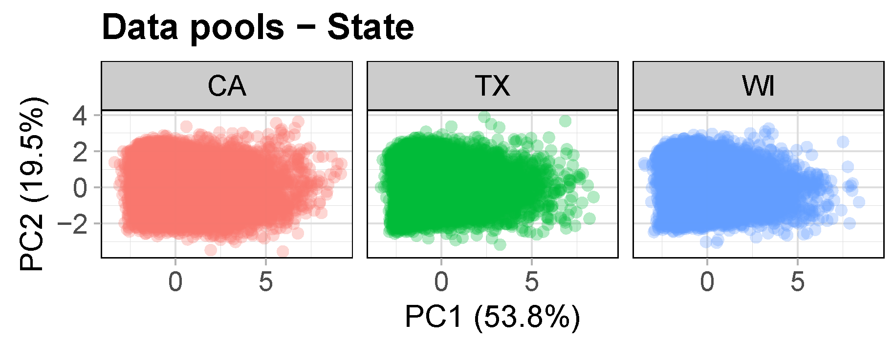
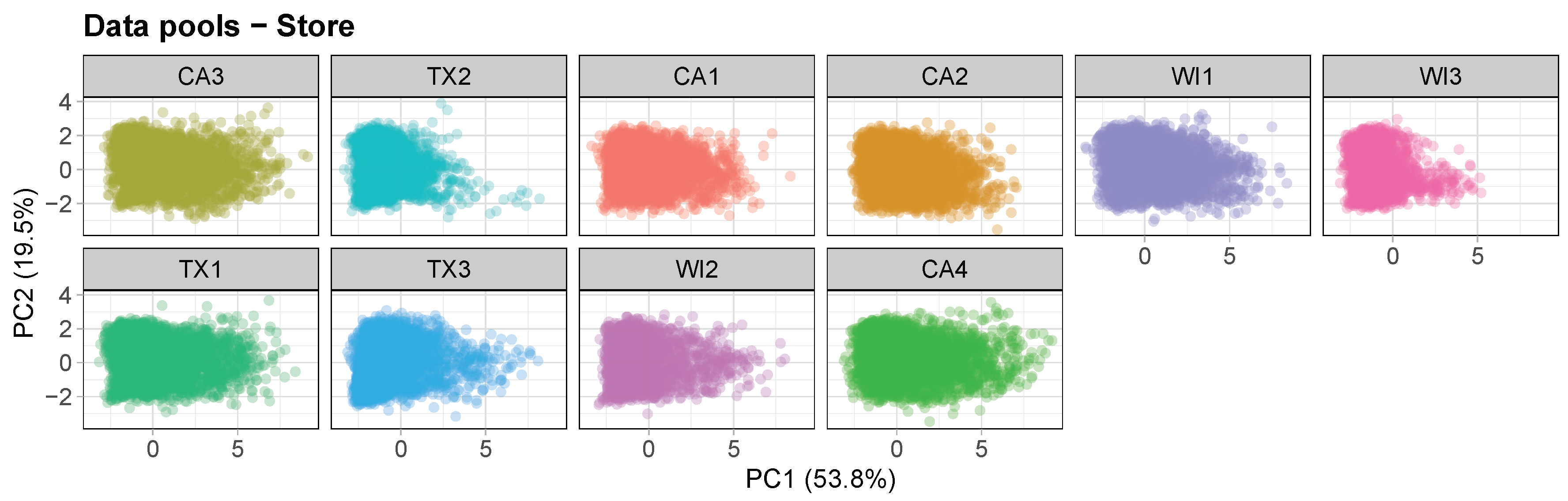
3.2. Data Pools
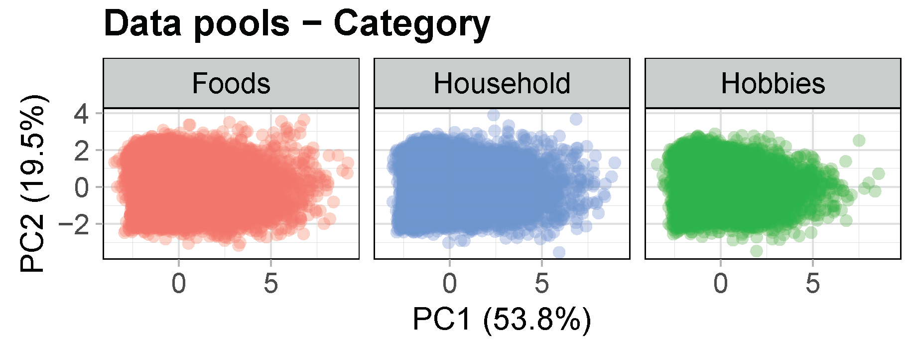
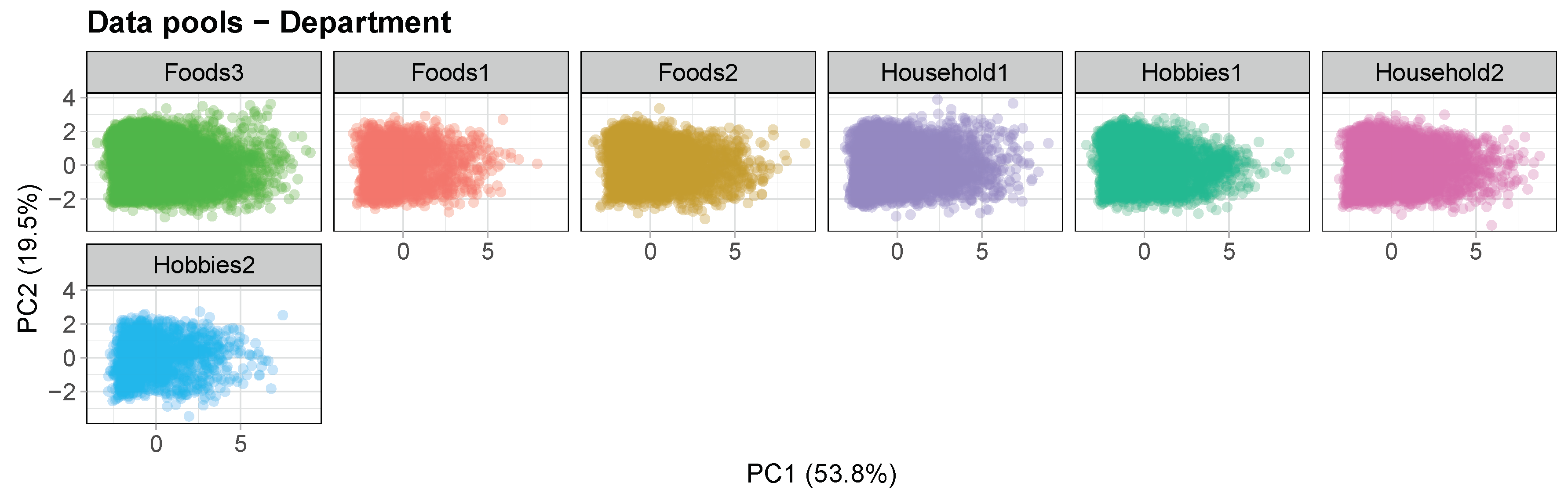
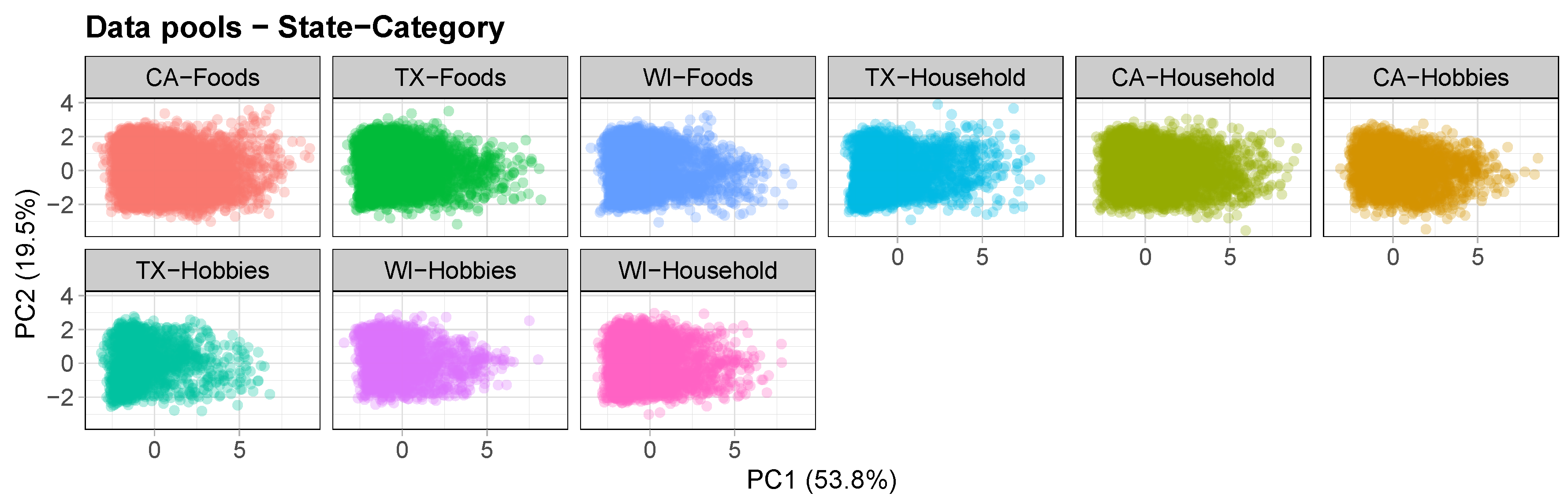
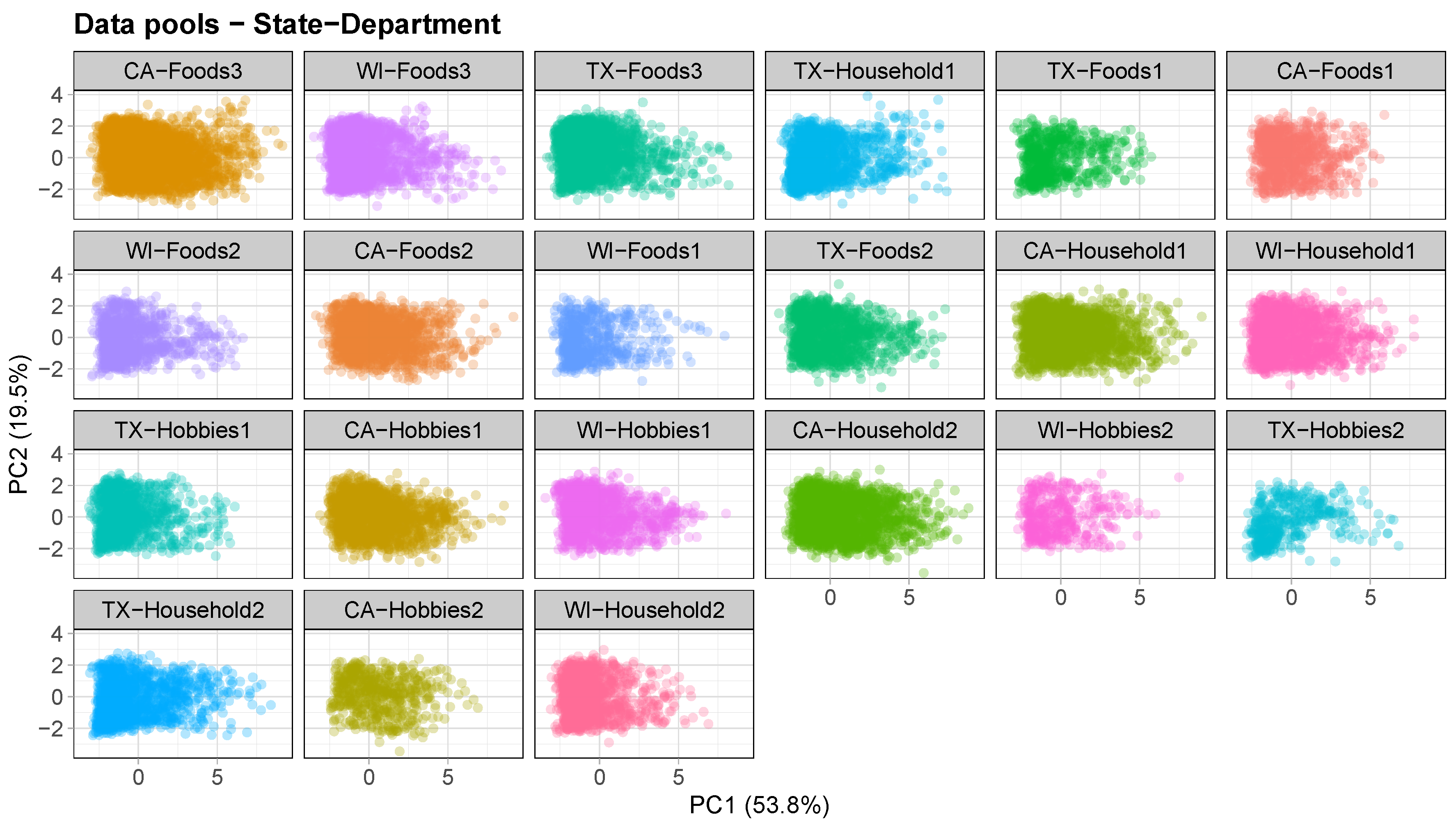
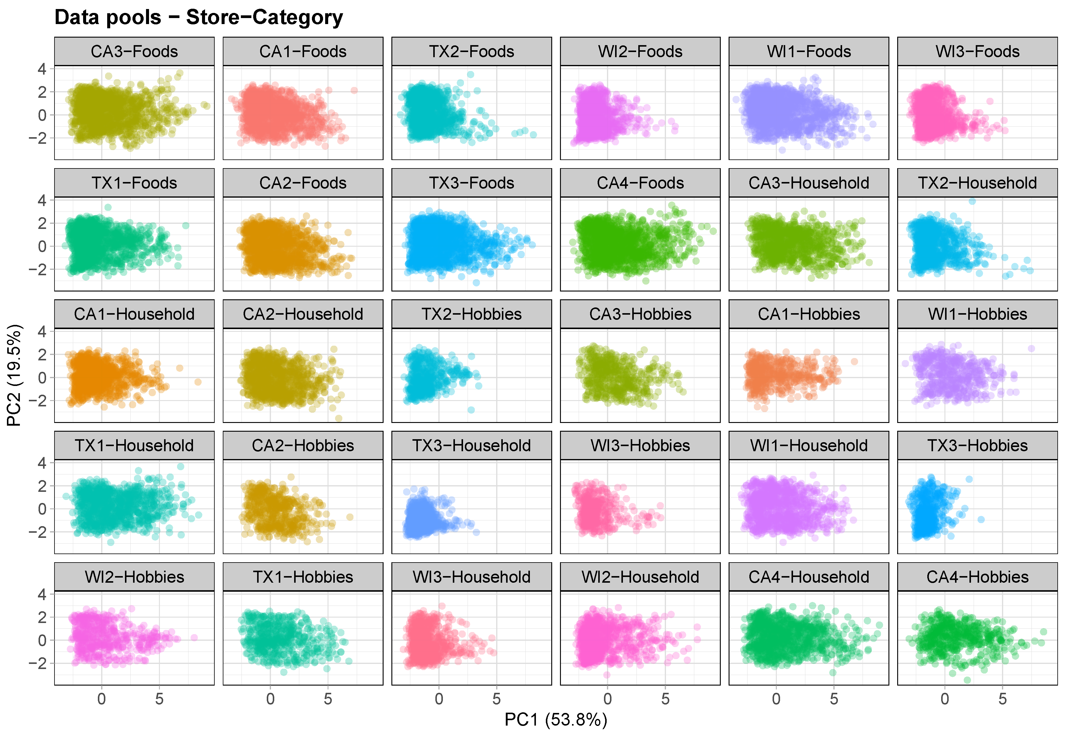
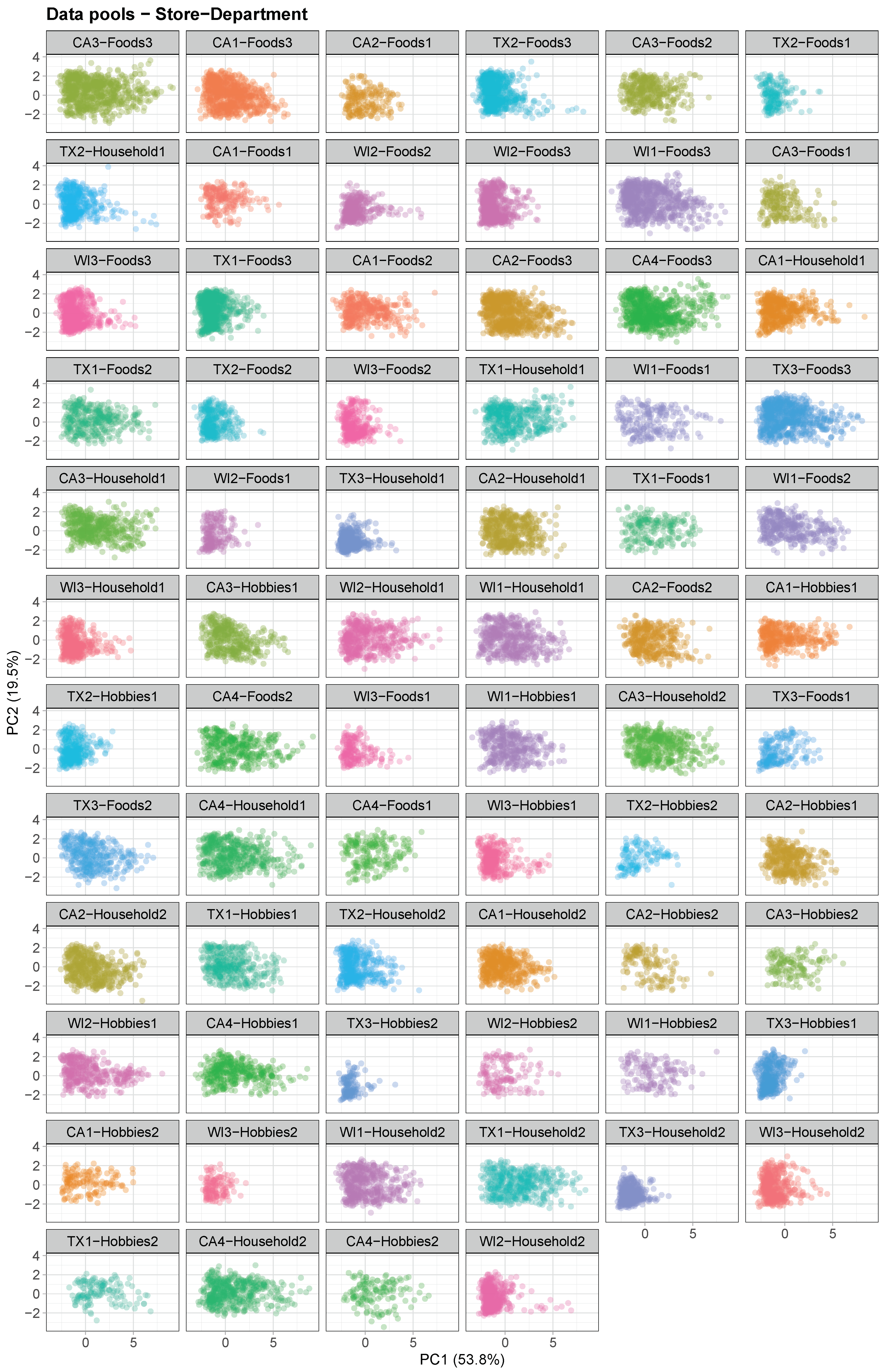
The approach used in the presented framework employs partial pooling and is inspired by the hierarchical structure of Walmart. The multi-level data provided are used to prepare five distinct levels of data, including total, state, store, category, and department, as well as four cross-levels of data, including state–category, state–department, store–category, and store–department. Data pools are then obtained for each level and cross-level. The total pool comprises the entire M5 dataset, which consists of 30,490 time series. At the state level, there are three data pools corresponding to the three states (CA, TX, and WI). CA has 12,196 time series, while TX and WI have 9147 time series each. The store level has ten data pools, including four stores in California (CA1, CA2, CA3, and CA4) and three stores in both Texas and Wisconsin (TX1, TX2, TX3, and WI1, WI2, WI3), each with 3049 time series. The category level has three data pools corresponding to the three distinct categories: Household, Hobbies, and Foods, each with a different number of time series (10,470 for Household, 5650 for Hobbies, and 14,370 for Foods). The department level has seven data pools, consisting of three departments for the Foods category (Foods1, Foods2, and Foods3) and two departments each for the Household and Hobbies categories. The number of time series in each department ranges from 1490 to 8230. The state–category cross-level consists of nine data pools, which result from crossing the three states with the three categories. For instance, CA–Foods contains the products from the Foods category that are available in CA stores. The number of time series in the state–category pools ranges from 1695 to 5748. Similarly, the state–department cross-level comprises 21 data pools that arise from the combination of the three states with the seven departments. For example, CA–Foods3 includes the products from the Foods3 department that are sold in CA stores. The number of time series in the state–department pools varies from 447 to 3292. The store–category cross-level has 30 data pools generated by crossing the ten stores with the three categories. For example, CA3–Foods includes the products from the Foods category that are sold in CA3 store. The number of time series in the store–category pools ranges from 565 to 1437. Lastly, the store–department cross-level has 70 data pools that arise from the combination of the ten stores with the seven departments. For instance, CA3–Foods3 comprises the products from the Foods3 department that are sold in CA3 store. The number of time series in the store–department pools ranges from 149 to 823. All this information is provided in
Appendix A.
It is noteworthy that we examined all feasible combinations of partial pools from the multi-level data available. We expect that as the sizes of the data pools decrease and the relatedness of the time series within them increases, the global models’ performance will improve, while their complexity will decrease. It is expected that the cross-learning scenarios developed, driven by the product hierarchy employed by the retailer, will result in improved global models that can capture interdependencies among products and regions more effectively. By utilizing data pools at the state and store levels, it may be possible to better understand cross-region dependencies and the impact of demographic, cultural, economic, and weather conditions on demand. Additionally, category and department data pools have the potential to uncover cross-product dependencies and improve the relationships between similar and complementary products. This partitioning method is simpler to implement than the current literature-based clustering methods that rely on feature extraction to identify similarities among the examined series.
3.3. Model Selection
A deepAR model was trained using all the time series available in each data pool, regardless of any potential heterogeneity. For instance, a deepAR model was trained for each state, namely CA, TX, and WI, making a total of three different models for the state level. Similarly, one deepAR model was trained for each store, resulting in ten distinct deepAR models for the store level, and so forth. Moreover, in the case of the total pool, only one deepAR model was trained, using the entire M5 dataset, which consists of 30,490 time series. As a result, a total of 154 separate deepAR models were trained, with each data pool having one model. Although complete pooling, which involves using a single forecasting model for the entire dataset, can capture interdependencies among products and regions, partial pooling, which uses a separate forecasting model for each pool, is often better suited for capturing the unique characteristics of each group.
We followed the structure of the M5 competition, which kept the last 28 days of each time series as the testing set for out-of-sample evaluation (23 May 2016 to 19 June 2016), while using the remaining data (29 January 2011 to 22 May 2016, 1941 days) for training the models. It is essential to find the appropriate model that can perform well during testing in order to achieve the highest possible level of accuracy. Typically, a validation set is employed to choose the most-suitable model. The effectiveness of a deep learning model largely depends on various factors such as hyperparameters and initial weights. To select the best model, the last 28 days of in-sample training from 25 April 2016 to 22 May 2016 were used for validation. The hyperparameters and their respective ranges that were utilized in model selection are presented in
Table 2. The Optuna optimization framework [
46] was used to carry out the hyperparameter optimization process by utilizing the Root Mean Squared Error (RMSE) [
4] as the accuracy metric for model selection. For both ARIMA and ETS local benchmarks, a model was chosen for each time series using the AICc value, resulting in a total of 30,490 models.
3.4. Model Complexity
Data partitioning based on relatedness enhances a dataset’s similarities, making it easier for a model to identify complex patterns that are shared across time series, thereby reducing the model’s complexity. Therefore, it is essential to have heuristics that can estimate the model’s complexity. As discussed in
Section 1.3, one way to do this is by counting the number of parameters (NP) in the model of the data pool and measuring the size of the gzip compression (CMS-compressed model size) of its output file, expressed in bytes. Each parameter represents a degree of freedom that the model has to capture patterns in the data. The more parameters a model has, the more complex and flexible it is to fit a wide range of training data patterns. A model’s output file can be compressed to a small size if the information contained within it is relatively simple, indicating that the model is simple. Conversely, if the output file is difficult to compress and requires significant storage space, this suggests that the information contained within it is more complex, indicating that the model is more complex. To obtain the total number of parameters (TNP) for each partitioning approach, we added up the number of parameters (NP) in the model for each of its data pools. Similarly, we calculated the total compressed model size (TCMS) in bytes by summing the sizes of the gzip output file of the model for each of its data pools.
Additionally, it should be noted that the complexity of a learned model is affected not only by its architecture but also by factors such as the distribution and complexity of the data, as well as the amount of information available. With this in mind, we also computed the weighted average number of parameters (WNP) and the weighted average compressed model size (WCMS) per model for each partitioning approach, as shown below.
where
is the dataset size (number of time series),
n is the number of data pools of the partitioning approach, and
is the size of the data pool
i.
A conservative estimate for the number of parameters in both ARIMA and ETS local benchmark models was considered. For ARIMA, we assumed a maximum of 16 parameters, based on the highest possible orders for the autoregression and moving average polynomials (, , , ) as well as the variance of the residuals. In the case of ETS, we estimated a maximum of 14 parameters per model by taking into account the number of smoothing parameters (, , , and ), initial states (, , ), and the variance of the residuals. The TNP for both ARIMA and ETS models was calculated by multiplying the number of separate models (30,490 in total in this case study) by 16 and 14, respectively. As a result, the WNP per model for ARIMA and ETS are 16 and 14, respectively. To obtain the TCMS in bytes for these benchmark models, the sizes of the gzip output file for each individual model were added together. The WCMS per model can be calculated by dividing the TCMS by the number of models.
3.5. Evaluation Metrics
The performance of global and local models was evaluated with respect to two performance measures commonly found in the literature related to forecasting [
47], namely the average of the Mean Absolute Scaled Error (MASE) and the average of the Root Mean Squared Scaled Error (RMSSE):
where
is the value of item
i at time
t,
is the corresponding forecast,
n is the length of the in-sample training, and
h is the forecast horizon (28 days in this case study). RMSSE was employed to measure the accuracy of point forecasts in the M5 competition [
18]. MASE and RMSSE are both scale-independent measures that can be used to compare forecasts across multiple products with different scales and units. This is achieved by scaling the forecast errors using the Mean Absolute Error (MAE) or Mean Squared Error (MSE) of the 1-step-ahead in-sample naive forecast errors in order to match the absolute or quadratic loss of the numerator. The use of squared errors favours forecasts that closely follow the mean of the target series, while the use of absolute errors favours forecasts that closely follow the median of the target series, thereby focusing on the structure of the data.
3.6. Statistical Significance of Models’ Differences
The MASE and RMSSE errors can be used to conclude if there are any statistically significant differences in the models’ performance. First, a Friedman test is performed to determine if at least one model performs significantly differently. Then, the post-hoc Nemenyi test [
48] is used to group models based on similar performance. Both of these tests are nonparametric, meaning that the distribution of the performance metric is not a concern. The post-hoc Nemenyi test ranks the performance of models for each time series and calculates the mean of those ranks to produce confidence bounds. If the confidence bounds of different models overlap, then it can be concluded that the models’ performances are not statistically different. On the other hand, if the confidence bounds do not intersect, then it can only be determined which method has a higher or lower rank. The
nemenyi() function in the R package
tsutils [
49] was used to implement these tests, and a significance level of
was employed for all tests.
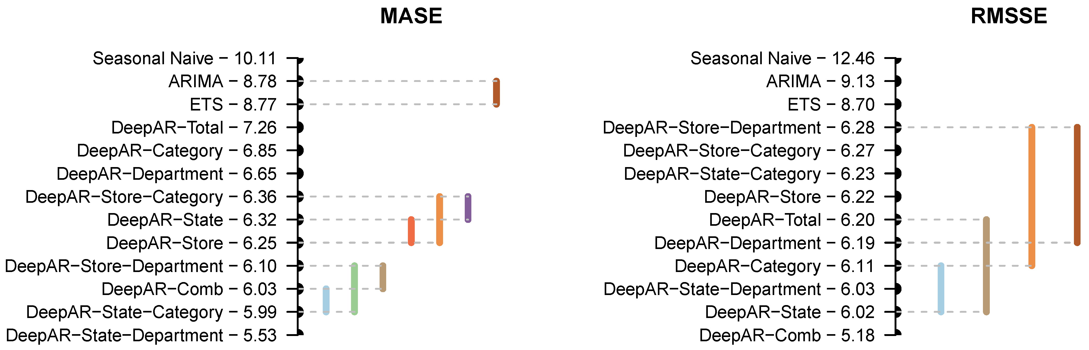
4. Results and Discussion
In this section, a comprehensive examination of the results achieved by the DeepAR global models of the various partitioning approaches and local benchmarks is presented. In addition to evaluating the forecast accuracy using MASE and RMSSE, a comparison of the complexities of the models is also provided. The results of the empirical study are presented in
Table 3 and
Appendix A.
Table 3 includes the percentage difference of each partitioning approach and local benchmark from DeepAR-Total in terms of MASE and RMSSE. This comparison aims to evaluate the enhancement achieved by partial pooling using the hierarchical structure of the data. Furthermore,
Appendix A exhibits tables that show the percentage difference of every data-pool model from the most-outstanding one within its aggregation level based on MASE and RMSSE. It is important to note that the results presented in these tables are ranked by MASE in each aggregation level.
Table 3 highlights the most-effective data-partitioning approach in boldface within the MASE and RMSE columns. In the field of forecasting, it is common to use forecast averaging as a complementary approach to using multiple models. Numerous studies have demonstrated the effectiveness of averaging the forecasts generated by individual models to enhance the accuracy of forecasts. Based on this idea, we computed the arithmetic mean of forecasts generated by the various partitioning approaches that were developed from the available data pools and denoted this as DeepAR-Comb.
The results presented in
Table 3 show that the data-partitioning approaches exhibit significantly better performance than the state-of-the-art local benchmarks. This finding suggests that global models are not inherently more limited than local models and can perform well even on unrelated time-series data. In other words, global models can increase model complexity compared to local models due to their generality. They can afford to be more complex than local models because they generalize better.
Overall, the partitioning approaches outperform DeepAR-Total across all levels of aggregation. DeepAR-State–Department achieves the highest performance according to MASE, while DeepAR-Comb performs best based on RMSSE (which can be explained by the use of RMSE as an accuracy metric for model selection).
Generally, the accuracy of data-partitioning approaches improves as the sizes of the data pools decrease. This can be attributed to the increased similarity among the time series in smaller pools, making it easier to capture cross-product and cross-region dependencies. As a result, models with lower complexity are needed when the data become less heterogeneous. We have observed that both the weighted average number of parameters (WNP) and the weighted average compressed model size (WCMS) decrease accordingly per model. As anticipated, the application of ARIMA and ETS to each time series individually leads to substantially lower WNP and WCMS values than those obtained with global models used in the data-partitioning approaches. The global models tend to be over-parameterised, with a higher number of parameters than training samples. In the case of WNP, the difference is four orders of magnitude higher, while in the case of WCMS, it is three orders higher.
We have observed that the performance gain of the partitioning approaches over DeepAR-Total is not significant, with an improvement of less than 1% based on RMSSE and up to 3.6% based on MASE. It is noteworthy that the DeepAR-State-Department approach, which uses only 21 data pools, outperforms the other approaches with a higher number of data pools (namely 30 and 70). This suggests that there is a trade-off between data availability and relatedness, where data partitioning can improve the relatedness and similarities between time series by increasing homogeneity. This allows for more-effective capture of the distinct characteristics of the set but at the cost of a reduced sample size, which has been proven to be harmful. Therefore, the primary goal should be to optimize this trade-off. Notably, in addition to achieving the highest forecasting accuracy, the DeepAR-State-Department approach exhibits the lowest weighted average number of parameters (WNP) and weighted average compressed model size (WCMS) per model.
By referring to
Appendix A, it can be observed that the DeepAR models associated with the Foods category or Foods1, Foods2, and Foods3 departments generally outperform the models of other categories/departments (see
Figure A3,
Figure A4,
Figure A5,
Figure A6,
Figure A7 and
Figure A8). This could be attributed to the higher proportion of non-zero demand (ratio between the number of non-zero observations and the total number of observations) in these data pools. However, it is not possible to establish a direct relationship between data homogeneity and model accuracy due to the different sizes of the data pools (with the exception of the Store level) and the different time series included in each data pool at each aggregation level.
Figure 2 presents the mean rank of the global and local models and the post-hoc Nemenyi test results at a 5% significance level for MASE and RMSSE errors, enabling a more-effective comparison of their performance. The forecasts are arranged by their mean rank, with their respective ranks provided alongside their names. The top-performing forecasts are located at the bottom of the plot. The variation in the ranks between
Table 3 and
Figure 2 can be explained by the distribution of the forecast errors. The mean rank is non-parametric, making it robust to outlying errors.
Once again, we have observed that global models outperform local benchmarks. Based on the MASE errors, there is no significant difference between ARIMA and ETS. In addition, DeepAR-State is grouped together with DeepAR-Store-Category and DeepAR-Store, while DeepAR-Comb does not differ from DeepAR-Store-Department and DeepAR-State-Category. The DeepAR-State-Department approach is ranked first and exhibits significant statistical differences from all other approaches. In a similar manner, there is evidence of significant differences among the other four models (DeepAR-Department, DeepAR-Category, DeepAR-Total, and Seasonal Naïve). With regard to the RMSSE, there is no evidence of statistically significant differences between DeepAR-Department, DeepAR-Total, DeepAR-Store, DeepAR-State-Category, DeepAR-Store-Category, and DeepAR-Store-Department. Likewise, DeepAR-State-Department is grouped together with DeepAR-Category and DeepAR-State, ranking on top. The remaining four models exhibit significant differences.
5. Conclusions
Retailers typically provide a wide range of merchandise, spanning from perishable products such as fresh produce to non-perishable items such as electronics and clothing. Each of these products exhibits unique demand patterns that can differ based on several factors, including location, time, day of the week, season, and promotional events. Forecasting sales for each product can be a daunting and complex undertaking, particularly given that retailers often sell through multiple channels, including physical stores, online platforms, mobile apps, and marketplaces. Furthermore, in the retail industry, demand forecasting is a routine task that is frequently conducted on a weekly or daily basis to maintain optimal inventory levels. Consequently, advanced models and techniques are required to address the forecasting challenge. These models must be automated to minimize manual intervention, robust enough to handle various data types and scenarios, and scalable to handle vast amounts of data and changing business conditions.
GFMs have shown superior performance to local state-of-the-art benchmarks in prestigious forecasting competitions such as the M4 and M5, as well as those on Kaggle with a forecasting purpose. The success of GFMs is based on the assumption that they are effective if there is a relationship between the time series in the dataset, but there are no established guidelines in the literature to define the characteristics of this relationship. Some studies suggest that higher relatedness between series corresponds to greater similarity in the extracted features, while others connect high relatedness with stronger cross-correlation and similarity in shapes or patterns.
To understand how relatedness impacts GFMs’ effectiveness in real-world demand forecasting, especially in challenging conditions such as highly lumpy or intermittent data, we conducted an extensive empirical study using the M5 competition dataset. We explored cross-learning scenarios driven by the product hierarchy, common in retail planning, to allow global models to capture interdependencies across products and regions more effectively.
Our findings demonstrate that global models outperform state-of-the-art local benchmarks by a significant margin, indicating their effectiveness even with unrelated time-series data. We also conclude that data-partitioning-approach accuracy improves as the sizes of data pools and model complexity decrease. However, there is a trade-off between data availability and data relatedness. Smaller data pools increase the similarity among time series, making it easier to capture cross-product and cross-region dependencies but at the cost of reduced information, which is not always beneficial.
Lastly, it is worth noting that the successful implementation of GFMs for heterogeneous datasets will significantly impact forecasting practice in the near future. It would be intriguing for future research to investigate additional deep learning models and assess their forecasting performance in comparison to the deepAR model.


