
YOLO-v5 Variant Selection Algorithm Coupled with Representative Augmentations for Modelling Production-Based Variance in Automated Lightweight Pallet Racking Inspection

Abstract
:1. Introduction
1.1. Literature Review
1.2. Paper Contribution
2. Methodology
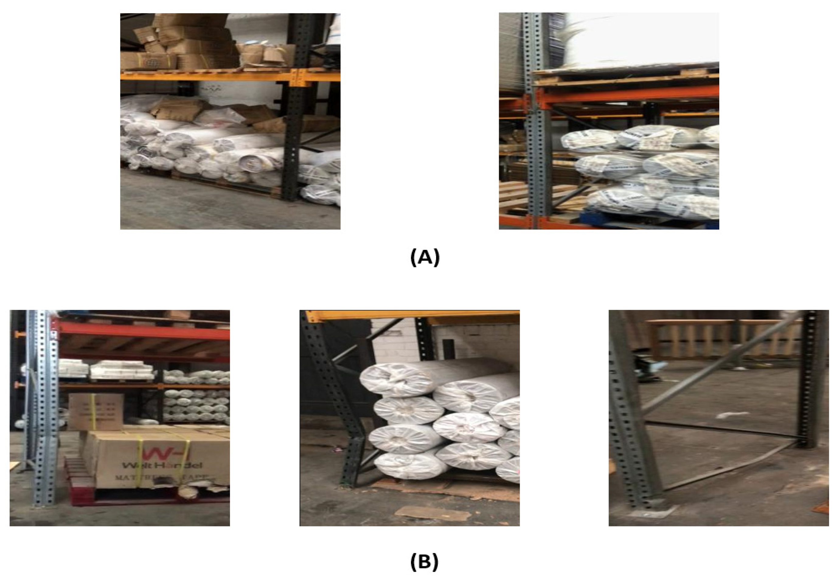
2.1. Dataset
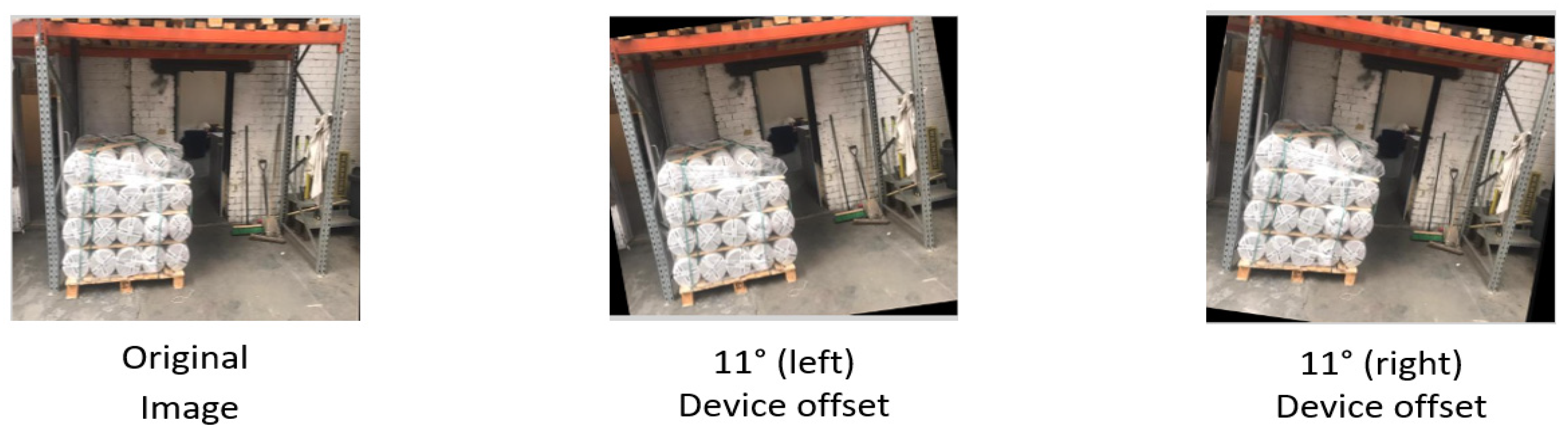
2.2. Domain-Inspired Augmentations
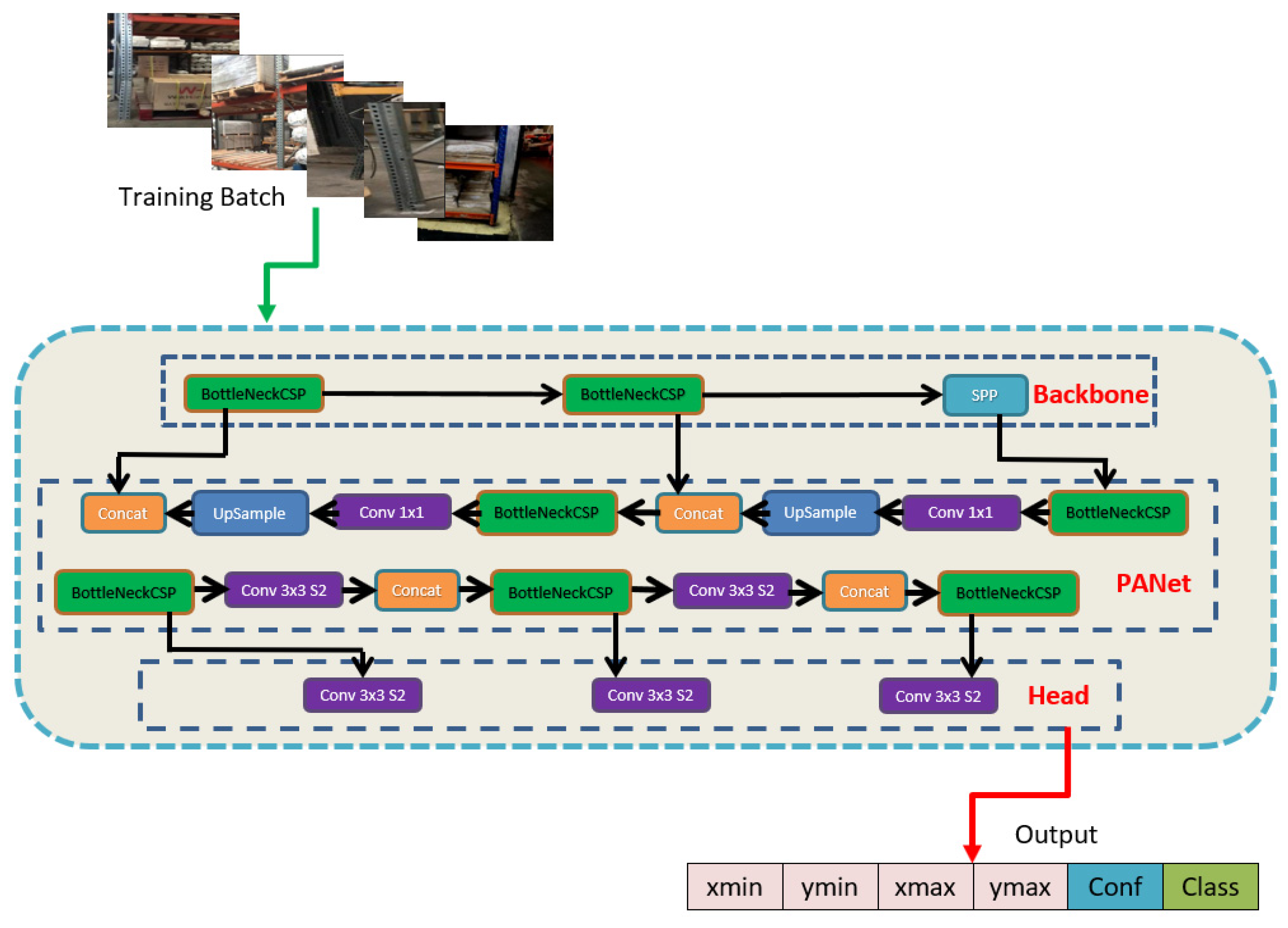
2.3. Proposed Architecture Selection Mechansim
2.4. Proposed YOLO-v5 Variant Selection Mechanism
3. Results
3.1. Hyperparameters
3.2. Performance Evaluation Metrics
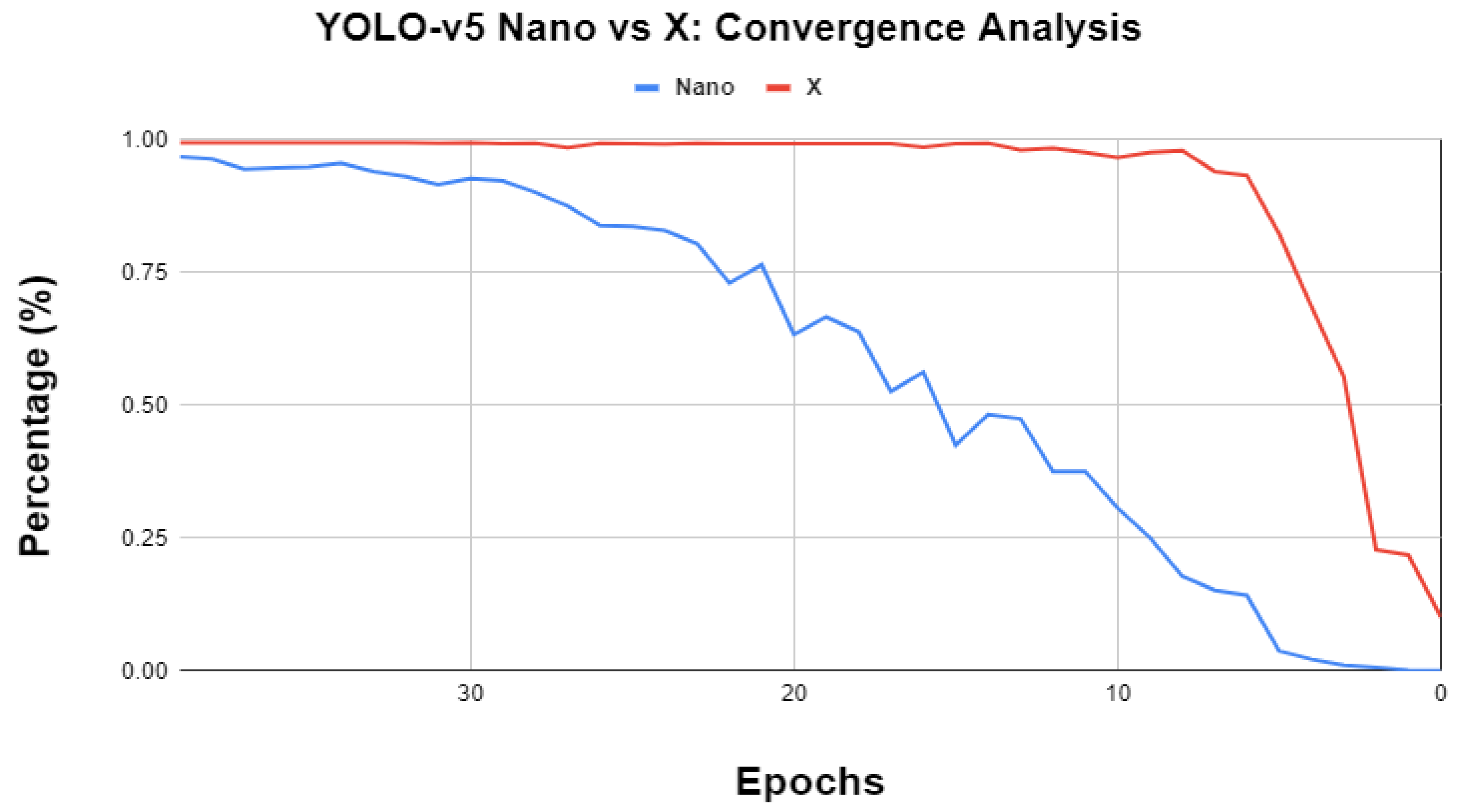
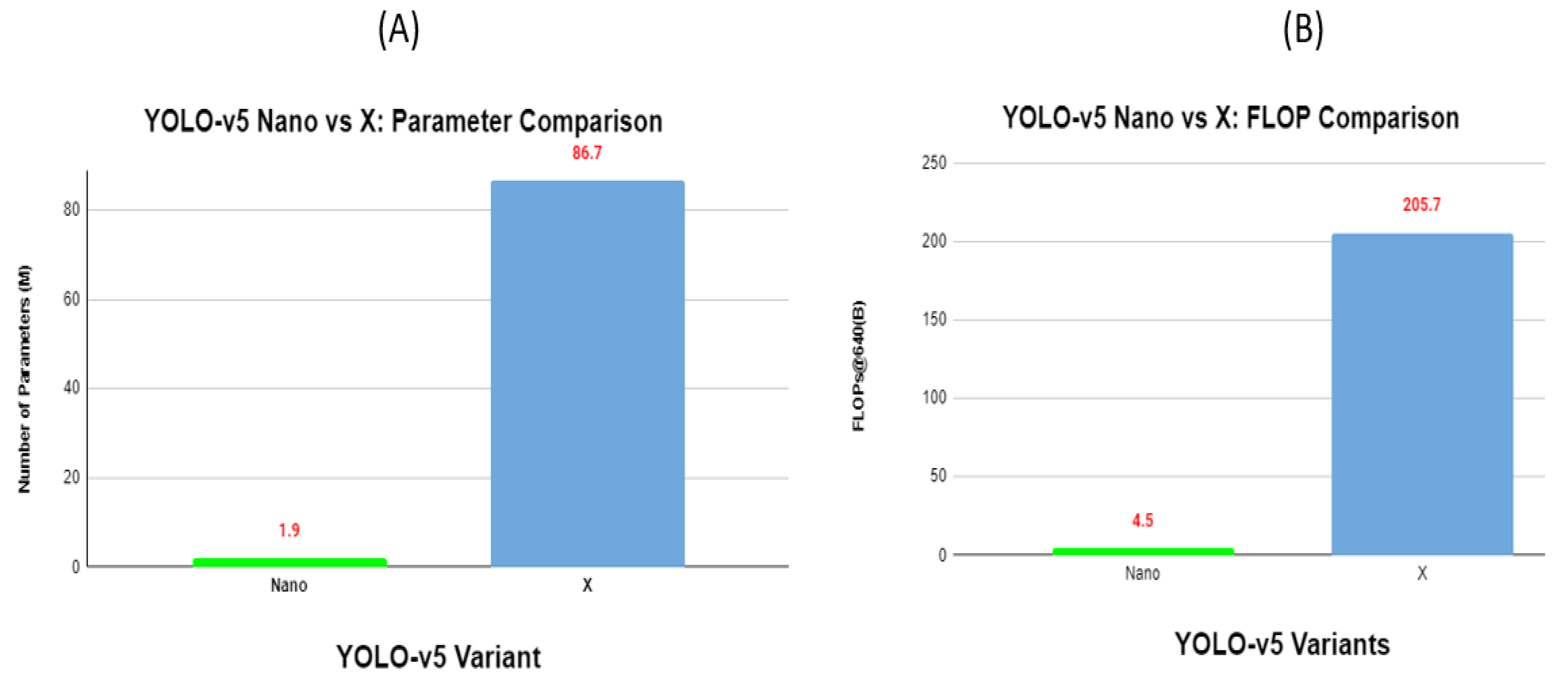
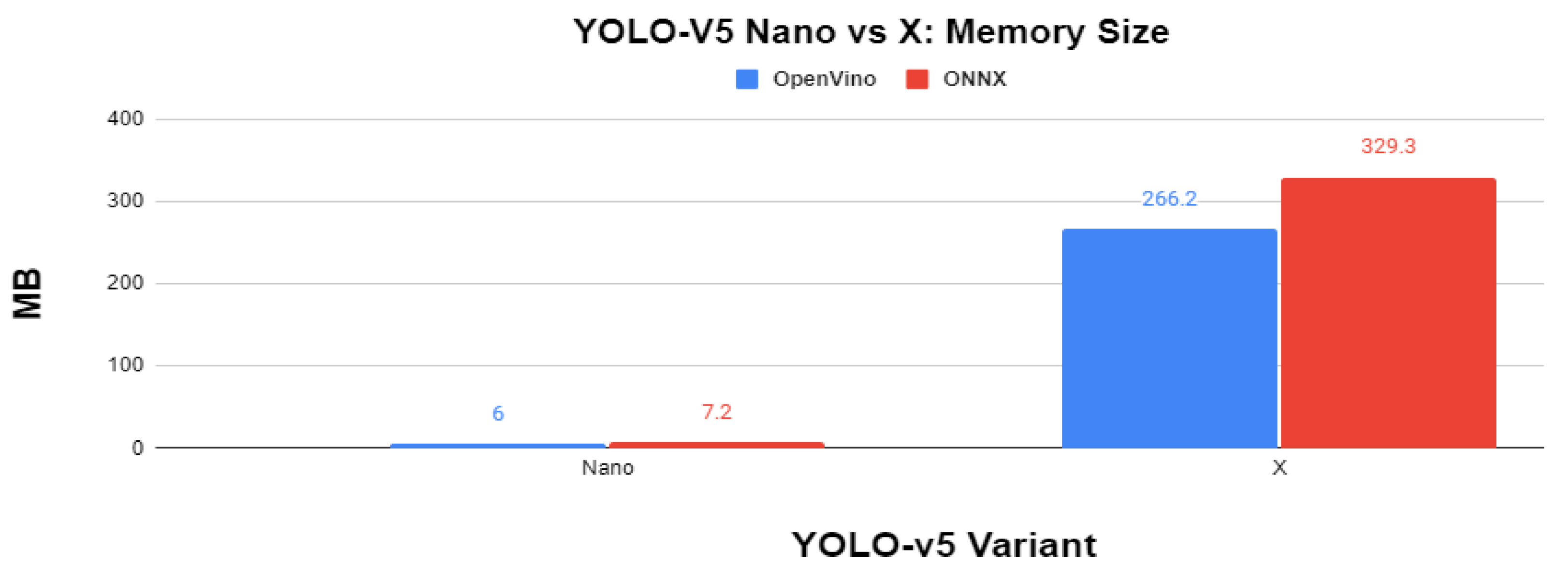
3.3. YOLO-v5 Extreme End Analysis
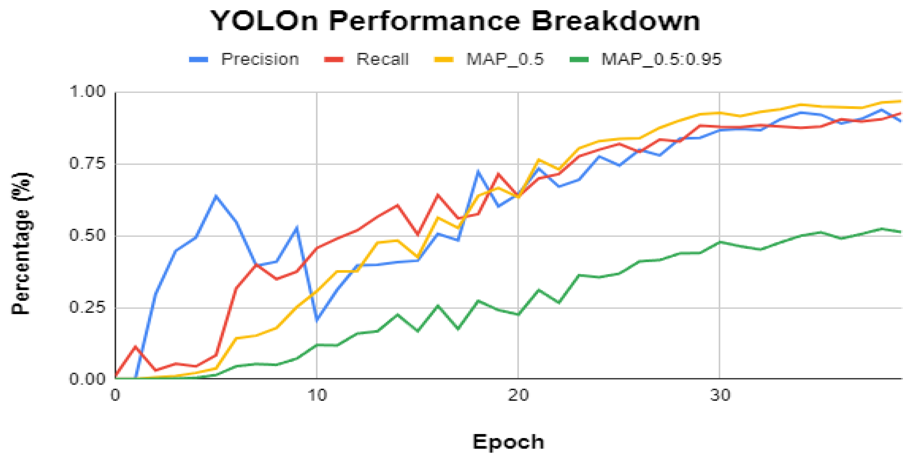
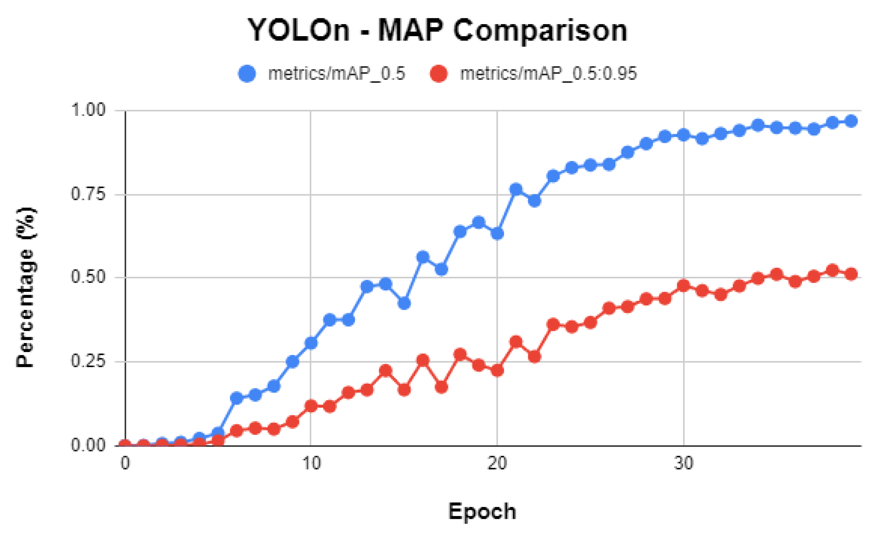
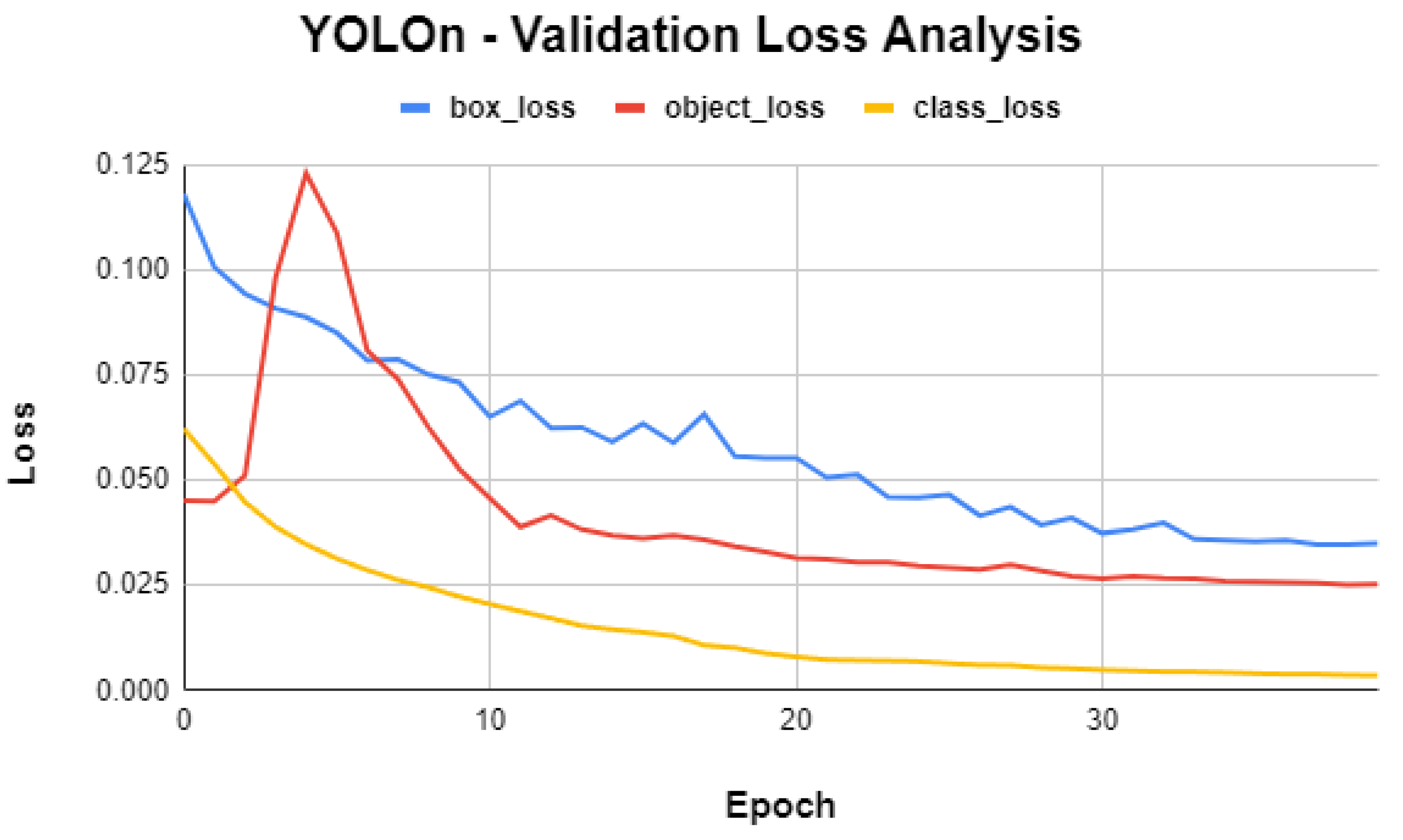
3.4. YOLO-v5n Detailed Performance Evaluation
4. Discussion
5. Conclusions
Funding
Data Availability Statement
Conflicts of Interest
References
- Aamer, A.M.; Islam, S.S. Distribution center material flow control: A line balancing approach. IOP Conf. Ser. Mater. Sci. Eng. 2019, 505, 012078. [Google Scholar] [CrossRef]
- Malik, H.; Chaudhary, G.; Srivastava, S. Digital transformation through advances in artificial intelligence and machine learning. J. Intell. Fuzzy Syst. 2022, 42, 615–622. [Google Scholar] [CrossRef]
- Alsboui, T.; Hill, R.; Al-Aqrabi, H.; Farid, H.M.A.; Riaz, M.; Iram, S.; Shakeel, H.M.; Hussain, M. A Dynamic Multi-Mobile Agent Itinerary Planning Approach in Wireless Sensor Networks via Intuitionistic Fuzzy Set. Sensors 2022, 22, 8037. [Google Scholar] [CrossRef] [PubMed]
- Chaouchi, H.; Bourgeau, T. Internet of Things: Building the New Digital Society. IoT 2018, 1, 1–4. [Google Scholar] [CrossRef] [Green Version]
- CEP, F.A. 5 Insightful Statistics Related to Warehouse Safety. Available online: https://www.damotech.com/blog/5-insightful-statistics-related-to-warehouse-safety (accessed on 11 March 2023).
- Warehouse Racking Impact Monitoring|RackEyeTM from A-SAFE. A-SAFE. Available online: https://www.asafe.com/en-gb/products/rackeye/ (accessed on 12 March 2023).
- Krizhevsky, A.; Sutskever, I.; Hinton, G.E. ImageNet classification with deep convolutional neural networks. Commun. ACM 2017, 60, 84–90. [Google Scholar] [CrossRef] [Green Version]
- Ran, H.; Wen, S.; Shi, K.; Huang, T. Stable and compact design of Memristive GoogLeNet Neural Network. Neurocomputing 2021, 441, 52–63. [Google Scholar] [CrossRef]
- He, K.; Zhang, X.; Ren, S.; Sun, J. Deep residual learning for image recognition. In Proceedings of the Conference on Computer Vision and Pattern Recognition, Las Vegas, NV, USA, 27–30 June 2016. [Google Scholar]
- Yang, Z. Classification of picture art style based on VGGNET. J. Phys. Conf. Ser. 2021, 1774, 012043. [Google Scholar] [CrossRef]
- Gajja, M. Brain Tumor Detection Using Mask R-CNN. J. Adv. Res. Dyn. Control Syst. 2020, 12, 101–108. [Google Scholar] [CrossRef]
- Liu, S.; Cui, X.; Li, J.; Yang, H.; Lukač, N. Pedestrian Detection based on Faster R-CNN. Int. J. Perform. Eng. 2019, 15, 1792. [Google Scholar] [CrossRef]
- Dong, C.-Z.; Catbas, F.N. A review of computer vision–based structural health monitoring at local and global levels. Struct. Health Monit. 2020, 20, 692–743. [Google Scholar] [CrossRef]
- Naseer, T.; Burgard, W.; Stachniss, C. Robust Visual Localization Across Seasons. IEEE Trans. Robot. 2018, 34, 289–302. [Google Scholar] [CrossRef]
- Hussain, M.; Al-Aqrabi, H.; Hill, R. PV-CrackNet Architecture for Filter Induced Augmentation and Micro-Cracks Detection within a Photovoltaic Manufacturing Facility. Energies 2022, 15, 8667. [Google Scholar] [CrossRef]
- He, Y.; Song, K.; Meng, Q.; Yan, Y. An End-to-End Steel Surface Defect Detection Approach via Fusing Multiple Hierarchical Features. IEEE Trans. Instrum. Meas. 2020, 69, 1493–1504. [Google Scholar] [CrossRef]
- Lal, R.; Bolla, B.K.; Sabeesh, E. Efficient Neural Net Approaches in Metal Casting Defect Detection. Procedia Comput. Sci. 2022, 218, 1958–1967. [Google Scholar] [CrossRef]
- Farahnakian, F.; Koivunen, L.; Makila, T.; Heikkonen, J. Towards Autonomous Industrial Warehouse Inspection. In Proceedings of the 2021 26th International Conference on Automation and Computing (ICAC), Portsmouth, UK, 2–4 September 2021. [Google Scholar] [CrossRef]
- Hussain, M.; Chen, T.; Hill, R. Moving toward Smart Manufacturing with an Autonomous Pallet Racking Inspection System Based on MobileNetV2. J. Manuf. Mater. Process. 2022, 6, 75. [Google Scholar] [CrossRef]
- Official Raspberry Pi Products|The Pi Hut. Available online: https://thepihut.com/collections/raspberry-pi/products/raspberry-pi-4 (accessed on 1 May 2023).
- Hussain, M.; Al-Aqrabi, H.; Munawar, M.; Hill, R.; Alsboui, T. Domain Feature Mapping with YOLOv7 for Automated Edge-Based Pallet Racking Inspections. Sensors 2022, 22, 6927. [Google Scholar] [CrossRef] [PubMed]
- He, K.; Zhang, X.; Ren, S.; Sun, J. Spatial pyramid pooling in deep convolutional networks for visual recognition. IEEE Trans. Pattern Anal. Mach. Intell. 2015, 37, 1904–1916. [Google Scholar] [CrossRef] [PubMed] [Green Version]
- Liu, S.; Qi, L.; Qin, H.; Shi, J.; Jia, J. Path aggregation network for instance segmentation. In Proceedings of the IEEE Conference on Computer Vision and Pattern Recognition (CVPR), Salt Lake City, UT, USA, 18–23 June 2018; pp. 8759–8768. [Google Scholar]
- Ansari, M.A.; Crampton, A.; Parkinson, S. A Layer-Wise Surface Deformation Defect Detection by Convolutional Neural Networks in Laser Powder-Bed Fusion Images. Materials 2022, 15, 7166. [Google Scholar] [CrossRef] [PubMed]
- Verstraete, D.; Ferrada, A.; Droguett, E.L.; Meruane, V.; Modarres, M. Deep Learning Enabled Fault Diagnosis Using Time-Frequency Image Analysis of Rolling Element Bearings. Shock Vib. 2017, 2017, 5067651. [Google Scholar] [CrossRef] [Green Version]


| Dataset | Samples |
|---|---|
| Training | 1905 |
| Validation | 129 |
| Model | Average Precision (@50) | Parameters | FLOPs |
|---|---|---|---|
| YOLO-v5s | 55.8% | 7.5 M | 13.2B |
| YOLO-v5m | 62.4% | 21.8 M | 39.4B |
| YOLO-v5l | 65.4% | 47.8 M | 88.1B |
| YOLO-v5x | 66.9% | 86.7 M | 205.7B |
|
train(YOLOv5nano, YOLOv5xtra,
, ): YOLOv5nano.train() YOLOv5xtra.train() nano_map = YOLOv5nano.evaluate() xtra_map = YOLOv5xtra.evaluate() while True: if xtra_map—nano_map > 0.05: YOLOv5nano = YOLOv5medium.train() new_map = YOLOv5nano.evaluate() if new_map—xtra_map > 0.05: YOLOv5nano = YOLOv5medium break else: xtra_map = new_map else: best_model = YOLOv5nano break if YOLOv5nano == YOLOv5xtra: break YOLOv5nano = next_variant(YOLOv5nano) nano_map = YOLOv5nano.evaluate() return best_model next_variant(model): if model == YOLOv5nano: return YOLOv5medium elif model == YOLOv5medium: return YOLOv5large elif model == YOLOv5large: return YOLOv5xtra else: return model |
| Epochs | 40 |
| Image Size | 640 |
| Cache | RAM |
| Device Type | GPU |
| Pretraining | IMAGENET |
| Model | MAP-IoU@0.5 | Parameters | FLOPs |
|---|---|---|---|
| YOLO-v5n | 96.8% | 1.9 M | 4.5B |
| YOLO-v5x | 99.4% | 86.7 M | 205.7B |
| Difference | 2.6% | 84.8 | 201.2B |
Disclaimer/Publisher’s Note: The statements, opinions and data contained in all publications are solely those of the individual author(s) and contributor(s) and not of MDPI and/or the editor(s). MDPI and/or the editor(s) disclaim responsibility for any injury to people or property resulting from any ideas, methods, instructions or products referred to in the content. |
© 2023 by the author. Licensee MDPI, Basel, Switzerland. This article is an open access article distributed under the terms and conditions of the Creative Commons Attribution (CC BY) license (https://creativecommons.org/licenses/by/4.0/).
Share and Cite
Hussain, M. YOLO-v5 Variant Selection Algorithm Coupled with Representative Augmentations for Modelling Production-Based Variance in Automated Lightweight Pallet Racking Inspection. Big Data Cogn. Comput. 2023, 7, 120. https://doi.org/10.3390/bdcc7020120
Hussain M. YOLO-v5 Variant Selection Algorithm Coupled with Representative Augmentations for Modelling Production-Based Variance in Automated Lightweight Pallet Racking Inspection. Big Data and Cognitive Computing. 2023; 7(2):120. https://doi.org/10.3390/bdcc7020120
Chicago/Turabian StyleHussain, Muhammad. 2023. "YOLO-v5 Variant Selection Algorithm Coupled with Representative Augmentations for Modelling Production-Based Variance in Automated Lightweight Pallet Racking Inspection" Big Data and Cognitive Computing 7, no. 2: 120. https://doi.org/10.3390/bdcc7020120