Article

Efficient Method for Continuous IoT Data Stream Indexing in the Fog-Cloud Computing Level

1
LabSTIC Laboratory, Department of Computer Science, 8 Mai 1945 University, Guelma 24000, Algeria
2
Technology Innovation Institute, Masdar City P.O. Box 9639, Abu Dhabi, United Arab Emirates
*
Author to whom correspondence should be addressed.
Big Data Cogn. Comput. 2023, 7(2), 119; https://doi.org/10.3390/bdcc7020119
Submission received: 9 May 2023 / Revised: 26 May 2023 / Accepted: 7 June 2023 / Published: 14 June 2023

Abstract

:
Internet of Things (IoT) systems include many smart devices that continuously generate massive spatio-temporal data, which can be difficult to process. These continuous data streams need to be stored smartly so that query searches are efficient. In this work, we propose an efficient method, in the fog-cloud computing architecture, to index continuous and heterogeneous data streams in metric space. This method divides the fog layer into three levels: clustering, clusters processing and indexing. The Density-Based Spatial Clustering of Applications with Noise (DBSCAN) algorithm is used to group the data from each stream into homogeneous clusters at the clustering fog level. Each cluster in the first data stream is stored in the clusters processing fog level and indexed directly in the indexing fog level in a Binary tree with Hyperplane (BH tree). The indexing of clusters in the subsequent data stream is determined by the coefficient of variation (CV) value of the union of the new cluster with the existing clusters in the cluster processing fog layer. An analysis and comparison of our experimental results with other results in the literature demonstrated the effectiveness of the CV method in reducing energy consumption during BH tree construction, as well as reducing the search time and energy consumption during a k Nearest Neighbor (kNN) parallel query search.

1. Introduction

IoT data is continually collected from a wide range of devices and sensors, which gives it some characteristics such as homogeneity within heterogeneity, data record size, time series format, dynamism [1], distribution and spatio-temporality [2] in addition to other big data characteristics [3]. These characteristics involve some issues, such as data overlapping and cloud computing latency, that make data searching and storage more difficult. To address these issues, many indexing methods for data storage have been proposed [4,5,6]. However, not all of the indexing methods are appropriate for the ever-changing IoT environment, due to the endless flow of heterogeneous IoT data. Before storage, the heterogeneous data streams in IoT must be processed and analyzed using novel methods appropriate to the evolutionary nature of the IoT environment. A novel process entails, in the first step, partitioning each IoT data stream into homogeneous groups, or clusters, before indexing in the second step. The data objects in each of the clusters are similar, but the clusters are dissimilar [7]. Several achievements in data stream clustering research [8,9] have been made. The current data stream clustering frameworks include four types of methods: partition-based, hierarchy-based, density-based and model-based methods [10]. Before being indexed in the second step, each cluster of the next data stream is compared to the existing clusters, and so on. The existing indexing structures for generating IoT data address the volume [11,12] and variety of types [13,14] but, in doing so, have limited efficiency. In comparison to multidimensional space, the metric space is ideal for addressing variety because it supports all types of data as long as its associated distance concept satisfies the triangular inequality. Metric Access Methods (MAMs) [15] can also be used to search for data in indexes in the metric space.
As a result of the progress in IoT device networking and communication, as well as some online applications and platforms, such as Google, Amazon, IBM, and Facebook, the architecture of the internet has become less efficient in supporting continuous streams of IoT and industrial IoT data, such as satellite imaging, social media, emails, and others. This large volume of data results in a significant processing load [16]. Thus, researchers have been using technological advancements and fog-cloud computing architecture to analyze and store massive amounts of IoT data. The cloud-computing layer, the fog-computing layer, and the terminal layer are all part of this architecture (Figure 1). The terminal layer is a multi-hop self-organizing sensors network made up of many nodes that are distributed throughout an area and frequently have wireless interconnection [17]. The fog-computing layer is located between the cloud and terminal layers. It is located at the network’s edge, close to the terminal layer [17]. The cloud computing layer is responsible for recovering and executing information derived from the other layers. A diverse set of applications can manage a large amount of heterogeneous IoT data in the cloud layer in a precise manner [18].
This paper proposes an effective approach in fog-cloud computing architecture. The aim is to overcome data volume problems, encountered in [11,12] and the variety of types [13,14], to organize and store the continuous flow of IoT data and to accelerate searches in the dynamic IoT environment. IoT data in the terminal layer is characterized by heterogeneity, noise, diversity, and rapid growth because it is collected from various devices [19]. The fog layer is divided into three levels for the organization of each IoT data stream: clustering fog level, clusters processing fog level, and indexing fog level (Figure 2). Density-Based Spatial Clustering of Applications with Noise (DBSCAN) is used for clustering at the fog level because it is the best algorithm for grouping diverse IoT data into homogeneous and high-density clusters. Outliers, or noise generated by data stream clustering, could be kept waiting for similar values from arriving streams. DBSCAN is an algorithm that is based on density accessibility and density connectivity. It requires two initial parameters: the cluster’s radius E p s and the minimum number of points M i n P t s [20].
Compared with other clustering algorithms, such as k-means [21] and Balanced Iterative Reducing and Clustering using Hierarchies(BIRCH) [22], DBSCAN can find irregularly shaped clusters, and is robust in detecting outliers [23]. Each cluster of the first data stream is stored in the cluster’s processing fog level and is directly indexed in the indexing fog level in a Binary tree with Hyper-plane (BH-tree). After DBSCAN clustering, the indexing of arrival data streams is based on a comparison of the arrival cluster’s coefficient of variation (CV) value and those of the arrival cluster’s unions with existing clusters in the clusters processing fog level. The arrival cluster is either directly indexed in a new BH-tree or inserted into an existing index, based on the minimum CV value. To assess its effectiveness, this approach is compared to two other scenarios. The fog layer in the IoT architecture is divided into only clustering and indexing levels in these scenarios. The first scenario, known as the Creation of a New Index (CNI) method, directly indexes data from each arrival cluster using a BH-tree. The second scenario, known as Insertion in an Existing Index (IEI) method, involves inserting data from each arrival cluster into an existing BH-tree.
The remainder of the paper is organized as follows. Section 2 introduces some methods for multidimensional and metric space clustering and indexing. Section 3 introduces the proposed approach with two scenarios for comparison and Section 4 describes the experimentation. The section on experimentation is divided into two parts. The first section describes the experimental platform and the datasets, while the second section presents, analyzes, and discusses the CV method’s experimental results, such as an evaluation of the BH-tree construction and the parallel kNN query search. Section 5 of the paper concludes with directions for future work.

2. Related Work

Existing approaches for indexing IoT data, whether in multidimensional [6,24,25,26,27] or metric space [28,29,30,31,32], do not provide efficient mechanisms for IoT data storage, despite their dynamic natures and continuous growth. There have been few publications in the field of continuous IoT data stream indexing. Wang et al. [33] proposed the Continuous Range Index (CR-index) as a method for indexing observed data, based on its value ranges and type attributes. The CR-index constructs a compact indexing scheme in which measurement and observation data items are aggregated into boundary blocks, based on their interval blocks. The indexes are designed to respond to range queries. This method, however, can only index data with a single dimension [2]. In [11], the authors presented a multi-attribute index combination. This method employs four types of attributes: spatial, temporal, keyword, and value. Each attribute has its indexing method, and the inclusion of these four indexes in a combined index necessitates a specific sequencing that determines the query search’s performance. By considering all possible sequences and automatically determining the most efficient combined index for each query, query search performance is improved. This approach focuses on improving query search performance, and the authors do not specify how to store indexed IoT data [11].
Doan et al. [34] introduced an indexing model for IoT data that includes a lossless compression technique as well as the advantages of bit-padding, bit-blocking, and Huffman coding. It reduces data size during compression, which eliminates the need for fixed eight-bit streams. The index is based on timestamps and allows access to compressed data without requiring full decompression. This information is linked in during the compression process. The goal of this framework was to create indexing within lossless compression for floating-point time series data. This framework, according to the authors, needs to be improved by addressing temporal alignment and de-duplication issues when IoT streaming data is sourced from multiple devices. In SeaCloudDM [35], continuous data generated by IoT devices is received, stored, and processed in a sea-computing layer. The sea-computing layer generates numeric key sample values that are much smaller than the original data from the devices. This key sample data is sent to the cloud data management layer to be processed later. To manage SQL queries and keyword searches, a combined Relational Data-Base and Key-Value (RDB–KV) store cloud data management model is used. However, because this method manages massive amounts of data from disparate sensors in the cloud, it suffers from latency issues. The methods mentioned above have limitations that limit their effectiveness. The CR-index’s unique dimension renders it useless for higher-dimensional data [33]. Given the use of a multi-attribute index, this method is not applicable to all data types [11]. The use of indexes based on timestamps adapt this method to a specific type of data [34]. The SeaCloudDM [35], like other cloud methods, suffers from latency issues, making it insufficient when processing continuous big IoT data.
To avoid these limitations during the indexing of the continuous data stream, we use the fog-cloud architecture to reduce latency in this work. The current approach is developed in the metric space, due to its ability to process data of various types and dimensions, as only distances between objects are used in this space. The fog layer is divided into three levels in the proposed approach: the clustering fog level, the clusters processing fog level, and the indexing fog level. In the clustering fog layer, the first arrival data are grouped into homogeneous clusters using the DBSCAN algorithm. These clusters are stored in the clusters processing fog layer, and their objects are indexed in the indexing fog layer in a Binary tree with Hyper-plane (BH-tree). Objects in the clusters processing fog level are indexed or inserted in existing BH-trees based on the value of the coefficient of variation (CV) in the clusters processing fog level. The division of continuous data into groups, or clusters, of similar objects may greatly aid in indexing. For example, Balakrishna et al. [36] proposed the Incremental Clustering Driven Automatic Annotation for IoT Streaming Data (IHC-AA-IoTSD). It is an automatic annotation mechanism for streaming semantic data generated by IoT sensors using incremental hierarchical clustering. SPARQL queries are used to extract semantic annotations from hierarchical clustered data. This mechanism, according to the authors, can be improved by using a hash table (key–value pair) to store SPARQL queries. Furthermore, artificial intelligence systems require lightning-fast decisions. The IHC-AA-IoTSD has a total time complexity of T ( n ) = θ ( n 3 ) . Clusters are formed automatically in the DBSCAN algorithm [23], and outliers are easily detected and compared with objects in the next data stream.

3. Proposed Approach

IoT allows devices (sensors, actuators) to communicate and share information with one another. These devices are diverse, and they are typically deployed in distributed and dynamic environments across a large geographical area. These devices generate data in a variety of formats, including textual, numerical, streaming, and multimedia data [2]. Due to the dynamism and diversity of types and dimensions, storing these continuous streams of IoT data and determining an efficient retrieval method involve significant challenges. The cloud-fog computing architecture (Figure 1) is used for the storage and indexing of the continuous IoT data stream, and is located in the terminal layer. Geographically dispersed IoT devices generate massive amounts of diverse data on a continuous basis. The indexing of this continuous data stream is carried out in the fog computing layer due to its numerous characteristics, such as reduction of service latency, provision of real-time applications, and the processing capacity of a large number of nodes [37].
The fog layer is divided into three levels in this work: clustering fog level, clusters processing fog level, and indexing fog level (Figure 2). Each data stream from the terminal layer is grouped into homogenous clusters at the clustering fog level. The first data stream’s clusters are stored in the clusters processing fog layer, and their objects are directly indexed in separate BH-trees in the indexing fog layer. In the clusters processing fog level, a new BH-tree is constructed for the arrival data streams. On the basis of the coefficient of variation (CV) value of the clusters, or objects, the arrival cluster is inserted into an existing BH-tree. The additional work introduced in each layer has no effect on the processing capabilities of fog nodes because the number of sensors installed automatically gives rise to a suitable type of hardware to capture, process, and transmit data from the sensors. This means that having many sensors requires a lot of power from the fog (this condition is ensured during the installation process). Furthermore, the Fog’s three-level architecture, with level specialization, allows for smoother processing. Detailed descriptions of the clustering, CV, and indexing methods are presented in the following sections. The definitions of the parameters used in this approach are regrouped in Table 1.

3.1. Clustering Method
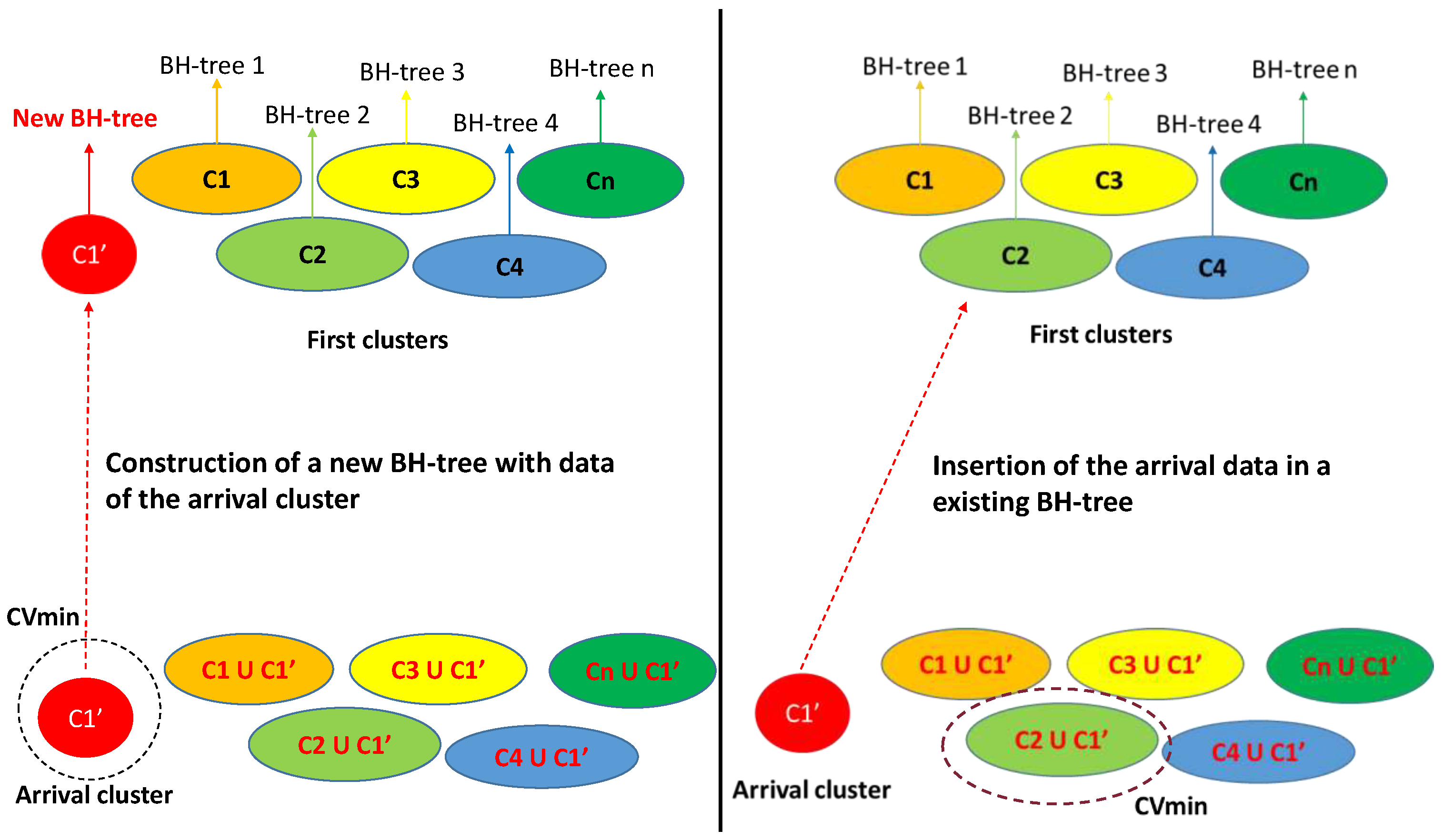
In the clustering fog level, each data stream sent by the terminal layer is collected and grouped in N clusters C l n with { n = 1 . . . N } . The Density-Based Spatial Clustering of Applications with Noise (DBSCAN) algorithm [38] is used. It is modified by the introduction of the calculation of the cluster centers ( c n ) for the coefficient of variation (CV). Each cluster C l n contains similar elements. Since Fog nodes do not have the same storage and processing capacities, the triggering of the clustering process is closely related to the storage capacity. This condition allows one to move beyond congestion and conceptual bottlenecks and tailor processing to the capabilities of the fog node.
The DBSCAN algorithm is one of the most used data clustering methods [7], based on the connection of points within a specific distance threshold. However, it only connects points that meet a density threshold (the number of objects in a radius). The DBSCAN algorithm divides the data into arbitrarily shaped clusters. Each cluster contains all the objects connected by the density. This clustering method was chosen because DBSCAN clusters form automatically, whereas the k-means algorithm, for example, requires the number of clustersto be determined before clustering. Furthermore, the DBSCAN algorithm is robust in the detection of outliers, which are considered to be objects that wait for other similar objects in the next data stream. The complexity of the DBSCAN algorithm for grouping a dataset of o objects into N clusters is O ( o . d ) [39] where, o = o c 1 + o c 2 + + o c N which could be written as o = N . m e a n ( o c ) , o c is the number of objects per cluster, and d is the average number of neighbors. This gives the final form of the DBSCAN algorithm’s complexity for each data stream, which is O ( N . m e a n ( o c ) . d ) .

3.2. CV Method

The coefficient of variation (CV) is used as a criterion in the clusters processing fog level to determine whether a cluster of the arrival data stream should be inserted in an existing BH-tree or indexed in a new BH-tree. The coefficient of variation is a statistical measure of data point dispersion around the mean in a dataset. It represents the standard deviation to mean ratio. The coefficient of variation has the advantage of being insensitive to data type and dimension [40]. The processing of the fog level clusters contains clusters from the first data stream C l n . Each cluster of the arrival data stream Cl k is unified with a copy of all the existing clusters C l n (Algorithm 1) at this fog level (Figure 3). Subsequently, the CV of the cluster of the arrival data stream CV Cl k and the CVs of the union of this cluster with every existing cluster CV Cl k C l n are determined. If the cluster of the arrival data stream Cl k has the minimum value of CV, a new BH-tree is constructed in the indexing fog level. The cluster Cl k is stored with the existing clusters C l n in the clusters processing fog level. If the minimum value of CV corresponds to the union of the cluster of the arrival data stream with an existing cluster Cl k C l n , objects in the arrival cluster Cl k are inserted into the BH-tree of the corresponding existing cluster C l n .
Since the CV calculation of the union of one arrival cluster with the first clusters is parallel, the complexity for all clusters is taken as the complexity for the CV calculation of the cluster with the maximum number of objects o c m a x . It represents approximately 2 m e a n ( o c ) and is given by O ( m e a n ( o c ) ) . Since the comparison of N arrival clusters with existing clusters is sequential, the complexity of the CV method for each data stream is O ( N . m e a n ( o c ) ) . The CV method processes clusters rather than data, which allows it to significantly reduce processing time, despite polynomial complexity, because the number of clusters is negligible in comparison to the number of data. This is due to the DBSCAN method’s capabilities, which allow it to detect all clusters, even those with a convex shape. The method, in fact, consider only true clusters, while the others are classified as noise.
Algorithm 1 CV method
Require:  C l = { C l 1 . . . C l n , n = 1 . . . N } Cl = { Cl 1 . . . Cl k , k = 1 . . . K }
Ensure:  I m
    for each data stream do
     for  cl Cl  do
         CV cl Calculate the coefficient of variation of the new cluster ( cl )
        for  c l C l  do
             CV cl c l Calculate the coefficient of variation of ( Cl C l )
            if  CV cl < CV cl c l  then
                create new index ( cl )
            else
                insert cl in I n
            end if
        end for
     end for
    end for

3.3. Indexing Method

The binary tree with hyper-plane (BH-tree) used in the indexing fog layer is based on a recursive division of space by a hyper-plane into two regions via two pivots p 1 , p 2 chosen as the two farthest elements. In the set E, elements closer to p 1 belong to the first region, while those closer to p 2 belong to the second region. This prevents regions from overlapping when answering queries. Firstly, a leaf node L N contains a subset E L N of objects with E L N E . Secondly, an inner node I N consists of two elements and two children: ( p 1 , p 2 , L , R ) O 2 × IN 2 . That is:
  • p 1 , p 2 are two unconfused objects, d ( p 1 , p 2 ) = d m a x , called “pivots”. They define the hyper-plane.
  • L is a left sub-tree and R is a right sub-tree.
The construction of the BH-tree is realized incrementally. The insertion is top–down.

3.4. The kNN Similarity Queries Search

The search algorithm gives an answer to query q with radius r q to recover the k objects closest to q (Algorithm 2). The set of k objects is stored in the list A. To address the queries, the kNN algorithm on the BH-tree is applied by starting from the root to its leaves. The search is performed by calculating the distance between the query point and the two pivots p 1 or p 2 , going down the tree, and determining whether the search should continue on the left branch (L) or the right branch (R). The query starts with a radius r q = + and, then, decrements by traversing each sub-tree that corresponds to the distance to the k e object in the order list A. Parallelism is also used in this work in the similarity search query process to minimize retrieve time to make the kNN search more efficient [39]. The complexity of the kNN search across all indexes could be reduced to the complexity of a single index search. The CV method is tested against two other scenarios to determine its effectiveness. The fog layer only contains the clustering and indexing levels in these scenarios. The first scenario is known as the Creation of a New Index (CNI) method, while the second is known as the Insertion into an Existing Index (IEI) method.
Algorithm 2 The kNN search in the BH-tree
kNN-BH-tree I N N , q R n , k N * , d : O × O R + , r q R + = + , A ( R + × O ) N = ( R + × O ) N
with:
( p 1 , p 2 , L , R ) = I N
d 1 = d ( p 1 , q )
d 2 = d ( p 2 , q )
B ( q , r q ) query ball q with radius r q
if  I N = = N U L L  then
    return A
else
    Calculate the distances d 1 and d 2
    if  | A | < k  then
        r q +
    else
        r A
    end if
    for  i ( 0 , 1 )  do
        if  d i < r q  then
             A k I n s e r t ( k , A , ( d i , p i ) )
        end if
        for each node I N  do
            if  B ( q , r q ) I N  then
                A k N N B H t r e e ( I N i , q , k , d , r q , A )
           end if
       end for
    end for
end if

3.4.1. CNI Method

Objects in the arrival data stream’s Cl are indexed in a new BH-tree in this scenario. Algorithm 3 includes a description of this method, which is straightforward, and there is no need to compare it to existing clusters or indexes. The CNI method generates indexes of objects that are similar.
Algorithm 3 CNI method
Require:  C l = { C l 1 . . . C l n , n = 1 . . . N }
     Cl = { Cl 1 . . . Cl k , k = 1 . . . K }
Ensure:  I n + k
    for each data stream do
        for  cl Cl  do
            create new index( cl )
        end for
    end for

3.4.2. IEI Method

Objects from each cluster of the arrival data stream are inserted into one of the existing indexes in this scenario. The cluster centers of the first data stream c n are used as representatives of the existing indexes in this method. The selection of an existing BH-tree into which the arrival cluster Cl objects are inserted is based on a distance test between the arrival cluster center c k and the existing BH-tree representative centers c n (Algorithm 4). When the distance between c k and c n is at a minimum, objects from the arrival cluster Cl are inserted in the index n.
Algorithm 4 IEI method.
Require:   C l = { C l 1 . . . C l n , n = 1 . . . N }
     Cl = { Cl 1 . . . Cl k , k = 1 . . . K }
Ensure:  I n
    for each data stream do
         for  cl k Cl  do
             for  cl n C l  do
                  M i n d calculate distances ( d ( c n , c k ) )
                 insert cl in I n
             end for
         end for
    end for

4. Experimentation

This section describes the experimental parameters, including the datasets and the experimental platform. Then, the experimental results regarding the evolution of the number of indexes with the data stream are discussed. The evaluation of the index construction and the evaluation of the parallel kNN search are also analyzed.

4.1. Experimental Settings

Three real data sets (GPS trajectory, WARD, and traffic datasets), and one synthetic dataset (Tracking), were used to test the four proposed indexing methods. The following subsections provide further information on these datasets.
  • GPS Trajectories: collected from Go!Track Android application [41]
  • Tracking dataset: moving vectors generated by an object tracking simulator with wireless cameras in the wireless multimedia sensor network in a random simulation [31]
  • Wearable Action Recognition Database (WARD): database of human action reconnaissance using wearable movement sensors [42]
  • Traffic dataset: belongs to the road network category [43]
The datasets were divided into subsets to perform the data stream simulation. The subsets of different sizes and dimensions (Table 2) were considered to be data streams. The experiments were carried out on a 64-bit Linux operating system (Ubuntu) with an Intel(R) Core TM i7-8550U CPU, 1.80 GHz × 8 processor, 16 GB RAM, and 256 GB ROM.

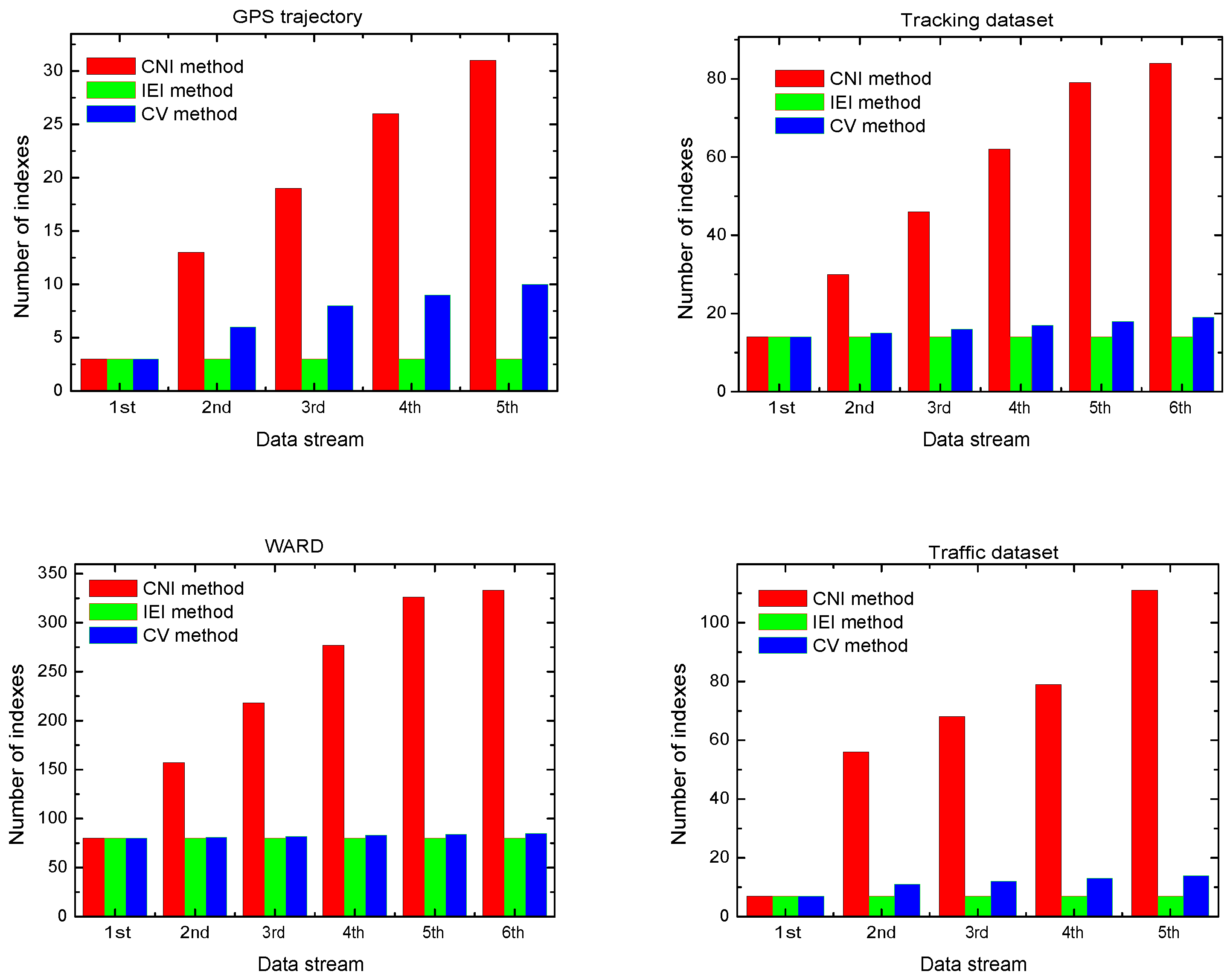
4.2. Evolution of the Number of Indexes with Data Stream

Figure 4 depicts the variation in the number of indexes as a function of the streams for the datasets used for the CV method and the other two scenarios. It is worth noting that the BH-tree of each cluster was constructed directly for the first data stream. For the second data stream, the proposed method was used. The IEI method, as expected, resulted in the construction of a minimum number of indexes that remained invariant with the data stream. Unlike the IEI method, the CNI method resulted in the construction of a maximum number of indexes that grew proportionally with the number of data streams. The number of constructed indexes for the CV method was between that of the IEI method and that of the CNI method. For all datasets, the number of indexes produced by the CV method was closer to that produced by the IEI method, indicating that the insertion process was more pronounced in the CV method than was the construction process. It can be noted that the number of indexes produced by the CV method varied from one data set to the next. This was directly dependent on the dynamic aspect of DBSCAN clustering, which caused the distances between cluster centers to change for each data stream.

4.3. Evaluation of Index Construction

The number of distances, comparisons, indexing time, and energy consumption were calculated as a function of the data stream to evaluate the BH-tree construction.

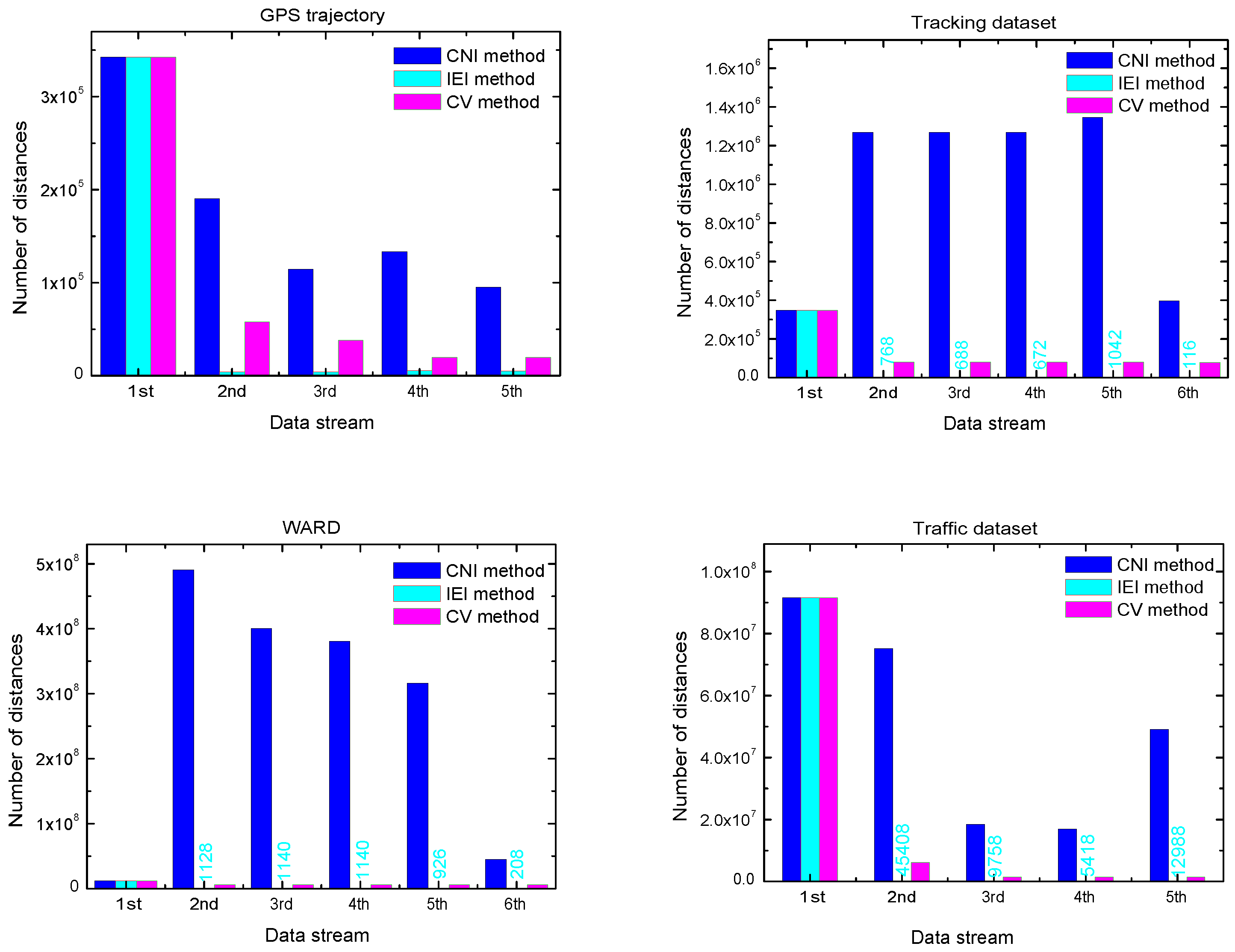
4.3.1. Number of Calculated Distances

As indicated in Figure 5, the number of distances was traced as a function of the data stream for the three methods. The number of distances during the construction of the BH-trees started varying from the second data stream. From this data stream, the number of distances varied, from one method to another, as a function of the data size. For the four datasets, the CNI method presented the highest number of distances, since the creation of pivots required more distance calculations, while the IEI method presented a lower number because, in the insertion process, no pivots were created. Despite the CV method combining both insertion and indexing processes, the number of distances, from this method, was close to that from the IEI method and this reflects the efficiency of the CV method.

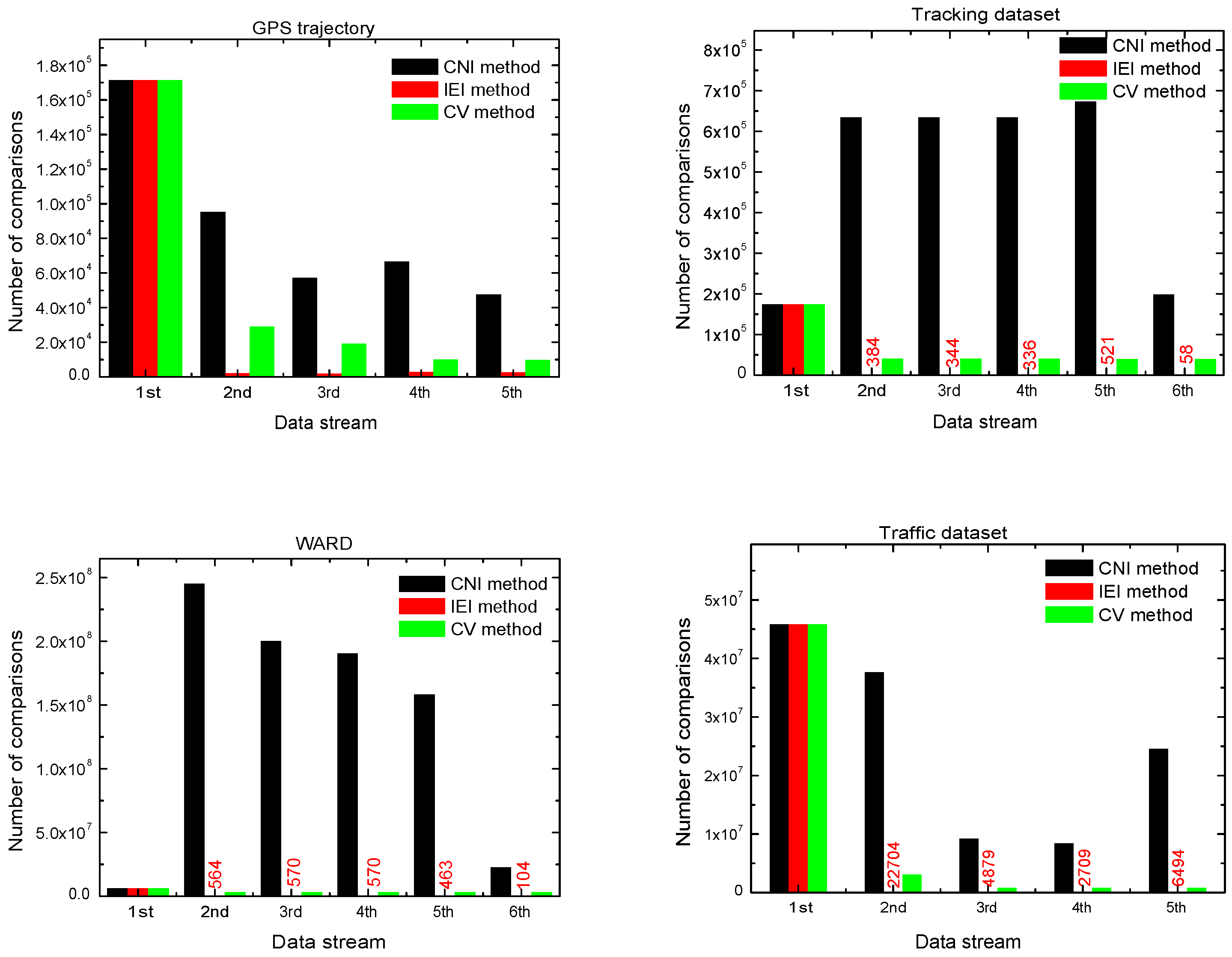
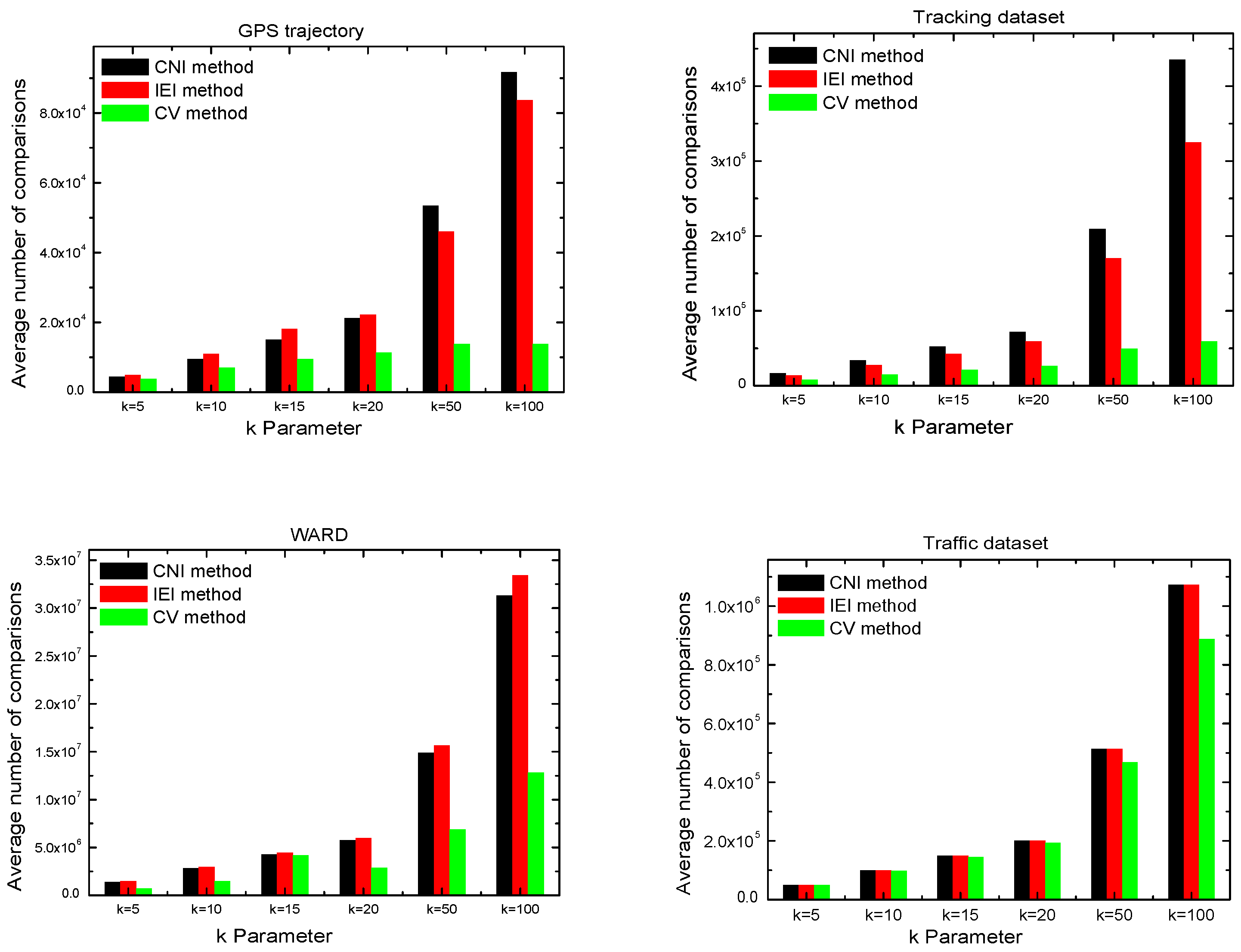
4.3.2. Number of Calculated Comparisons

Figure 6 depicts the variation in the number of comparisons as a function of the data stream. This variation, as seen in Figure 5, was similar to that of the number of distances. The number of comparisons was greater than the number of distances for all three methods. Comparisons were required during the construction of new indexes or during insertion to select the left or right side of each BH-tree.

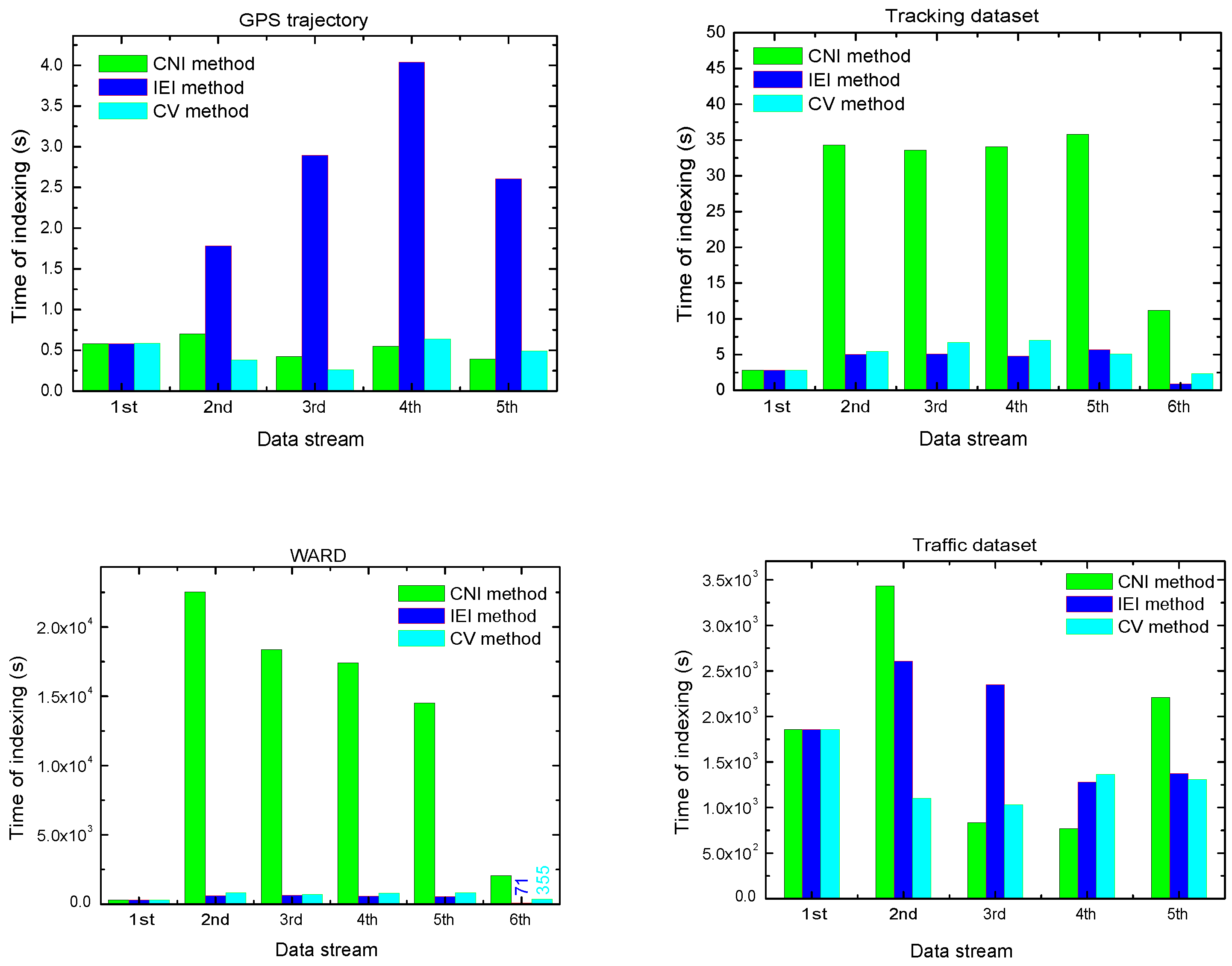
4.3.3. Indexing Time

As shown in Figure 7, indexing time depended not only on the data stream but also on the size of each data stream. For GPS trajectory data, the time of indexing was great when the IEI method was used, while for tracking and WARD data, the time of indexing was at a maximum when the CNI method was used. The time required to index the traffic dataset varied depending on the method used and the data stream. The indexing of data streams using the CV method consumed acceptable times for the four datasets used, regardless of data stream size. Unlike the IEI and CNI methods, the CV method was not affected by the size of the data stream.

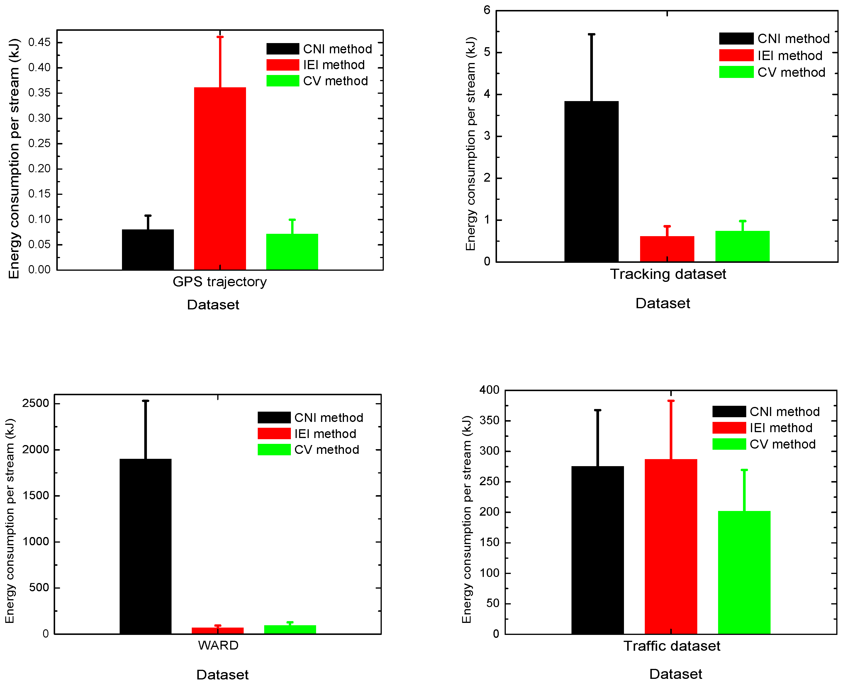
4.3.4. Energy Consumption during the Indexing

Figure 8 illustrates the energy consumption per stream for the CV, CNI and IEI methods. The energy consumption E p r o g (in Joule) during the execution of a program p r o g is given by the following expression [44]:
E p r o g = t b t e P ( p r o g , t ) d t t b t e P i ( t ) d t
where, t b and t e represent the beginning time and the end time of the execution of the program p r o g (in second), P ( p r o g , t ) is the electrical power needed for the execution of the program p r o g (in Watts) and P i ( t ) is the idle power (in Watts).
Figure 8 indicates that the energy consumed during indexing using these three methods varied depending on the dataset. The energy consumption for the GPS trajectory increased during data indexing using the IEI method. The energy consumption when using the CV method was lower than when using the CNI method. In contrast to the GPS trajectory dataset, the CNI method consumed more energy during the indexing of both tracking and WARD datasets than the CV and IEI methods. These last two were mostly close. The energy consumption during indexing using the CNI and IEI methods for the traffic dataset was comparable and greater than that during indexing using the CV method.

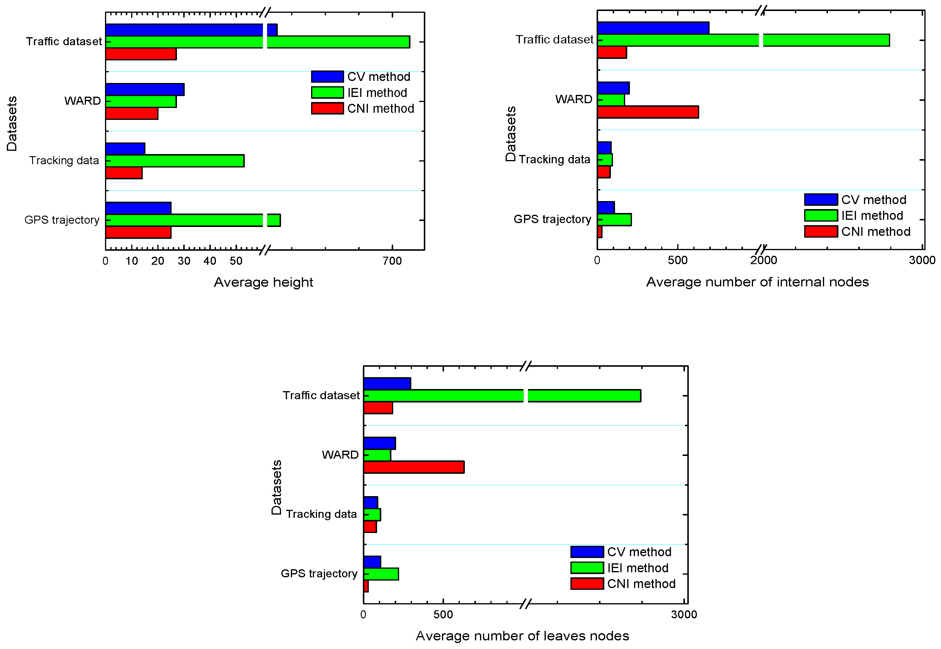
4.4. Quality of the Constructed BH-Trees

In Figure 9 the average height of indexes, the average number of internal nodes and the average number of leaves nodes are plotted for the four datasets to evaluate and compare the quality of BH-trees constructed using the CV method with those using the IEI and the CNI methods. The number of nodes per level (Figure 10) and the data distribution in leaves (Figure 11) were determined after the indexing of all data streams.

4.4.1. Average Height of BH-Trees

Figure 9 presents the average height of BH-trees resulting from the indexing of streams of GPS trajectory, tracking, WARD and traffic datasets. The average height of indexes constructed using the IEI method was greater than that of indexes constructed using the CNI method for all datasets. This was due to the fact that, in the IEI method, all data were inserted into a fixed number of BH-trees, whereas in the CNI method, a BH-tree was constructed for each cluster. In addition, Figure 9 shows that, for the GPS trajectory and tracking datasets, the average height of indexes constructed using the CV method was comparable to that of the CNI method, whereas for the WARD and traffic datasets, the average height from the CV method was greater than that of the CNI method and slightly exceeded the average height from the IEI method for the WARD data. The CV method’s behavior varied depending on the size and dimension of the data stream. When indexing the GPS trajectory and tracking datasets, it behaved similarly to the CNI method, and when indexing the WARD and traffic datasets, it behaved similarly to the IEI method.

4.4.2. Average Number of Internal Nodes

Figure 9 illustrates how the average number of internal nodes per BH-tree varied depending on the dataset. The average number of internal nodes in indexes constructed using the IEI method was greater than in indexes constructed using the CNI method for GPS trajectory, tracking, and traffic datasets, whereas for the WARD dataset, the average number of internal nodes in BH-trees constructed using the CNI method was greater than that in indexes constructed using the IEI method. The average number of internal nodes constructed using the CV method was located between those of the CNI and IEI methods for all datasets. The variation in the average number of leaves nodes as a function of the indexing method was similar to the variation in the average number of internal nodes, as expected (Figure 9).

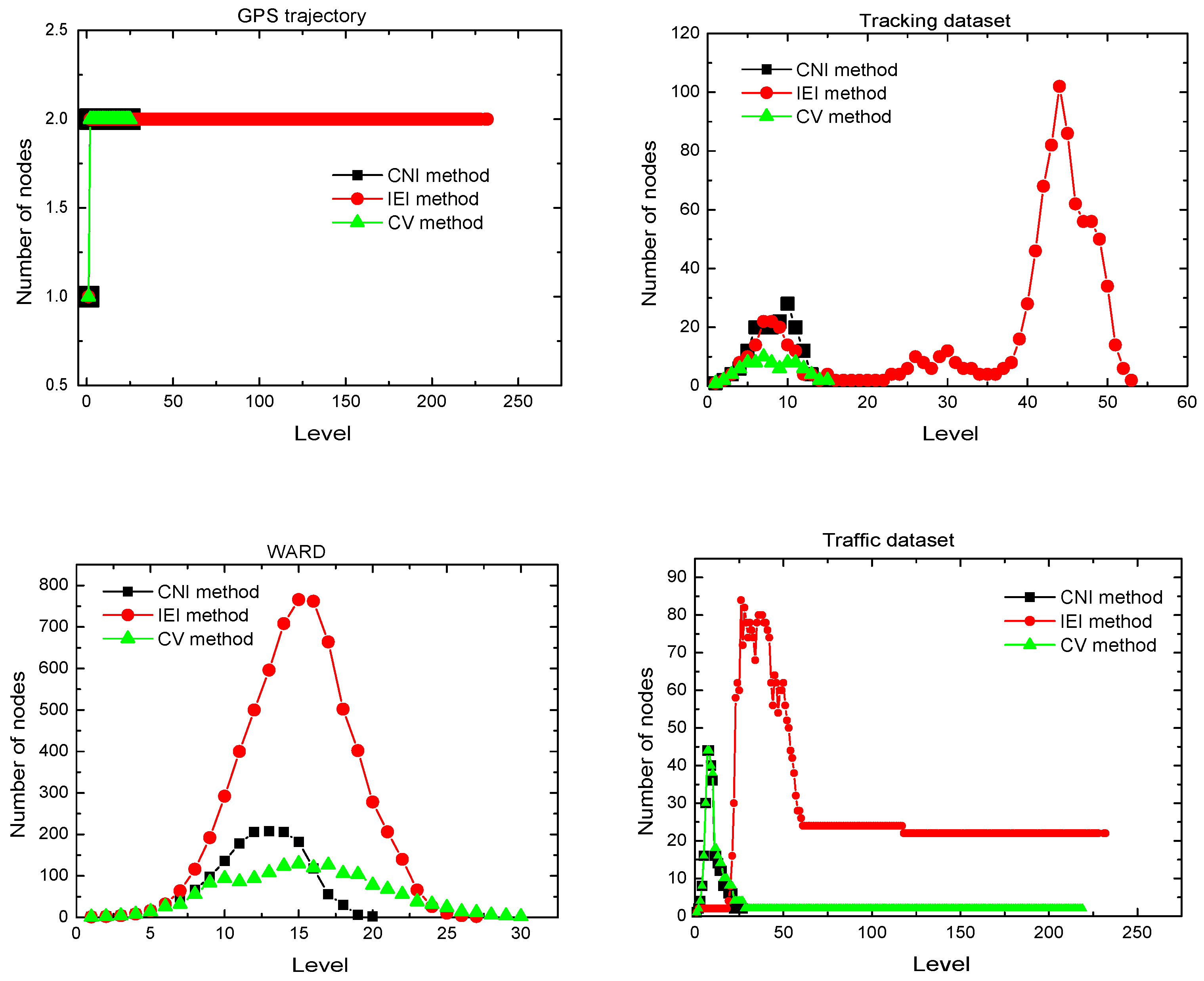
4.4.3. Number of Nodes per Level

Figure 10 depicts the number of nodes per level in BH-trees constructed using the CNI, IEI, and CV methods for the four datasets used. The number of nodes per level varied depending on the dataset, and the number of nodes in the GPS trajectory was constant at all levels of the BH-tree, regardless of the proposed indexing method. Moreover, the number of internal nodes per level in a tracking dataset varied depending on the indexing method. The IEI method yielded five levels with a high number of nodes, while the CV method yielded two levels with a high number of nodes and the CNI method yielded only one level with a high number of nodes from indexes. Only one level, with the maximum number of nodes in indexes constructed using both CNI and IEI methods, was used for the WARD dataset. The CV method produced indexes with two levels of maximum number of nodes. For the traffic dataset, BH-trees constructed using the CNI and CV methods yielded one level with the highest number of nodes. Three levels of the IEI methods had many nodes. Beyond level 25 for the CV method (2 nodes per level) and level 60 for the IEI method (25 nodes per level), the number of nodes remained constant.

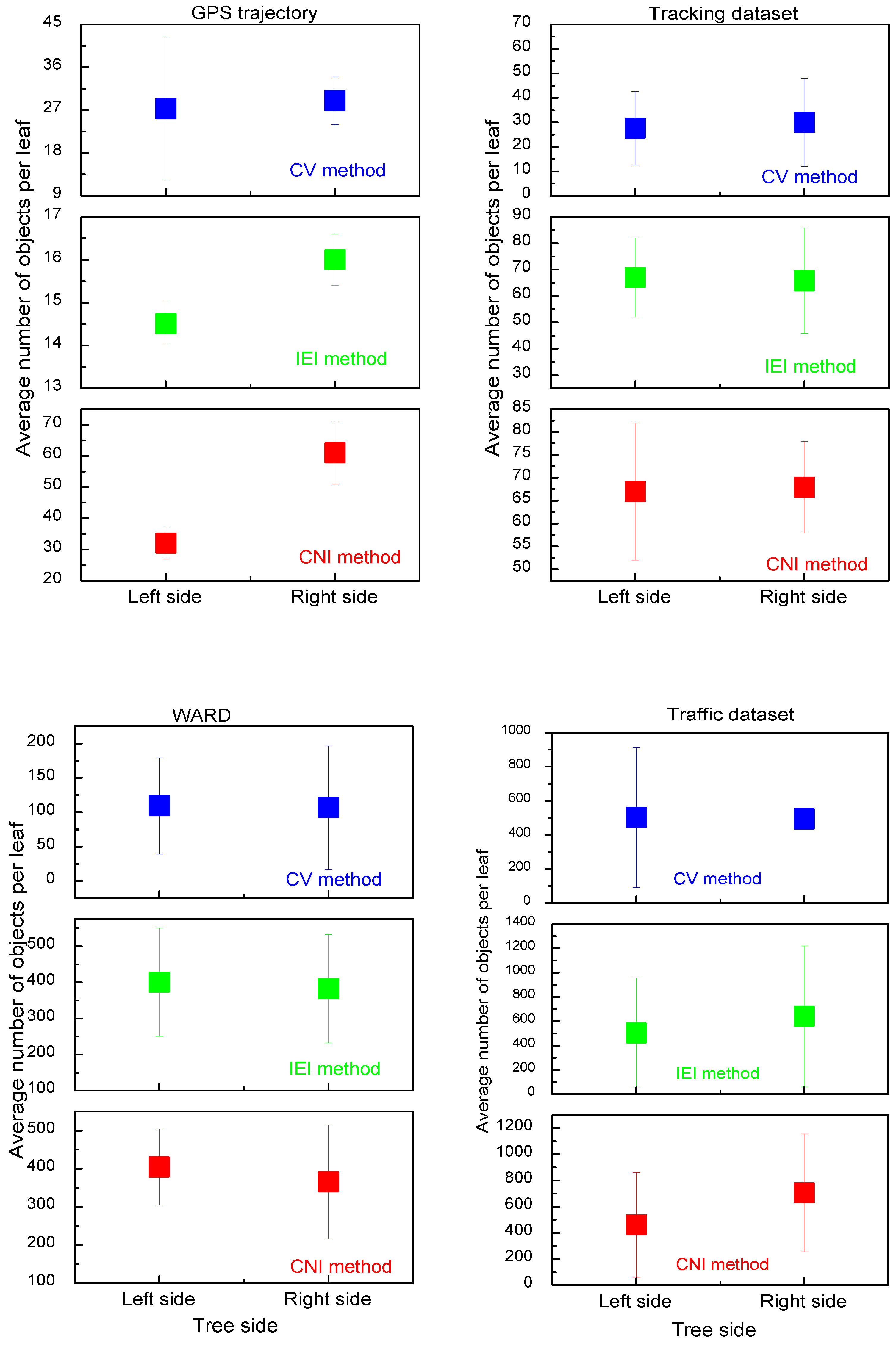
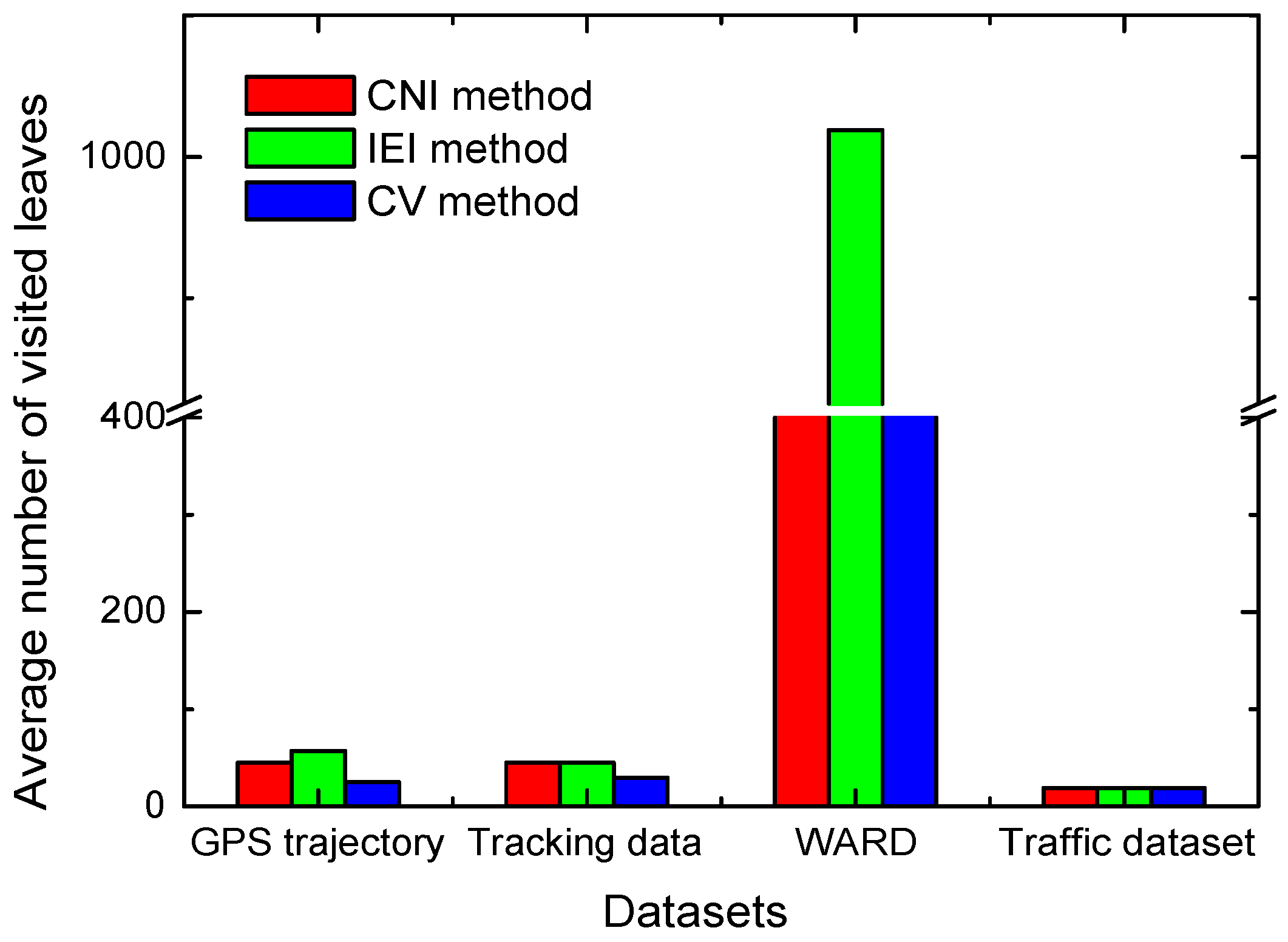
4.4.4. Data Distribution in BH-Tree Leaves

Figure 11 shows the data distribution for the CNI, IEI, and CV methods on the left and right sides of the BH-tree. The resulting indexes for GPS trajectory datasets constructed using both CNI and IEI methods were not balanced, whereas indexes constructed using the CV method were well balanced. Indexes from the three proposed methods were well balanced for the trajectory, WARD, and traffic datasets. It can also be noted that the data distribution in indexes built using the CNI and IEI methods was similar regardless of the dataset used.

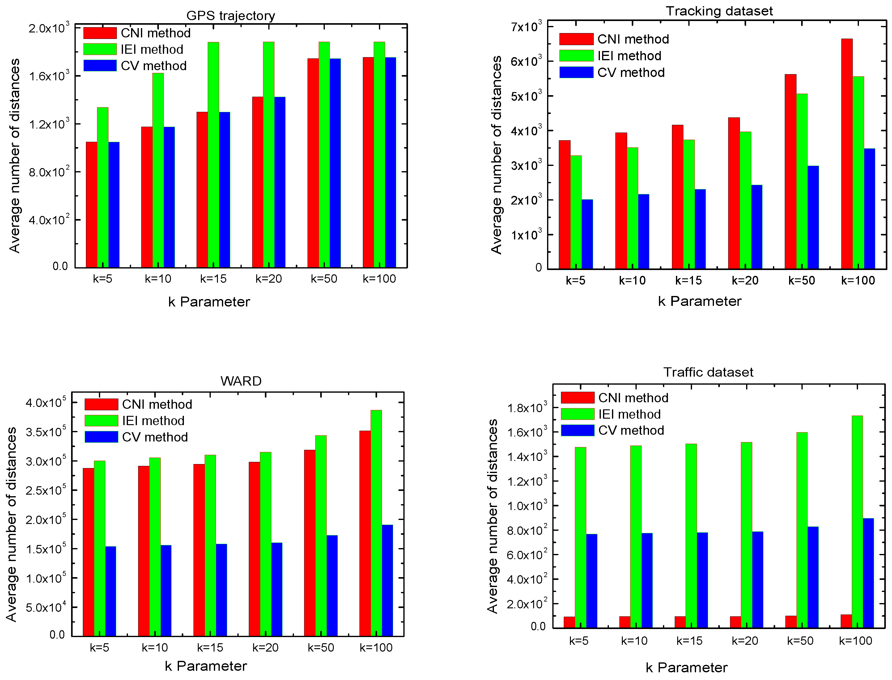
4.5. Evaluation of the Parallel kNN Search in BH-Trees

The number of distances, the number of comparisons, the time of search, energy consumption and the number of visited leaves were determined to search 100 queries to evaluate the parallel kNN search with k = 5 , 10 , 15 , 20 , 50 and 100 in BH-trees constructed using CNI, IEI and CV scenarios. All statistical results were averaged over 100 randomly generated queries.

4.5.1. Number of Calculated Distances

In Figure 12, the average number of calculated distances during the kNN search with k = 5 , 10 , 15 , 20 , 50 and 100 was plotted for the three methods. The average number of distances varied from data to data (Figure 12). The average number of distances calculated during the query search in BH-trees constructed using the CNI and CV methods for the GPS trajectory dataset was close to, and less than, that calculated during the query search in indexes constructed using the IEI method. As the number of nodes per level in the GPS trajectory data was constant (Figure 10) this could be related to the variation in average height of indexes (Figure 9). The average number of distances calculated during the kNN query search in indexes constructed using the CV method was less than the number of distances calculated in indexes constructed using the CNI and IEI methods for tracking and WARD data sets. This was due to the variation in the number of nodes per level (Figure 10). For the tracking dataset and levels between 5 and 10, the CNI method had more nodes than the IEI method, and the IEI method had more nodes than the CV method. The number of nodes per level from the IEI method was greater than that from the CNI method, which was greater than the number of nodes per level from the CV method for the WARD data set. For the traffic dataset, the number of distances calculated during the query search in CV method indexes was greater than that in CNI method indexes and less than that in IEI method indexes. This could be directly related to the height of the index (Figure 9).

4.5.2. Number of Calculated Comparisons

Figure 13 depicts the average number of comparisons calculated during the kNN queries search in BH-trees constructed using CNI, IEI, and CV methods. The four datasets exhibited similar variations. It can be noted that the average number of comparisons calculated in indexes built using the CV method was less than that calculated in indexes built using the CNI and IEI methods. This could be because the CV method resulted in the fusion of clusters of similar objects, as opposed to the IEI method, which inserted heterogeneous objects into a fixed number of indexes.

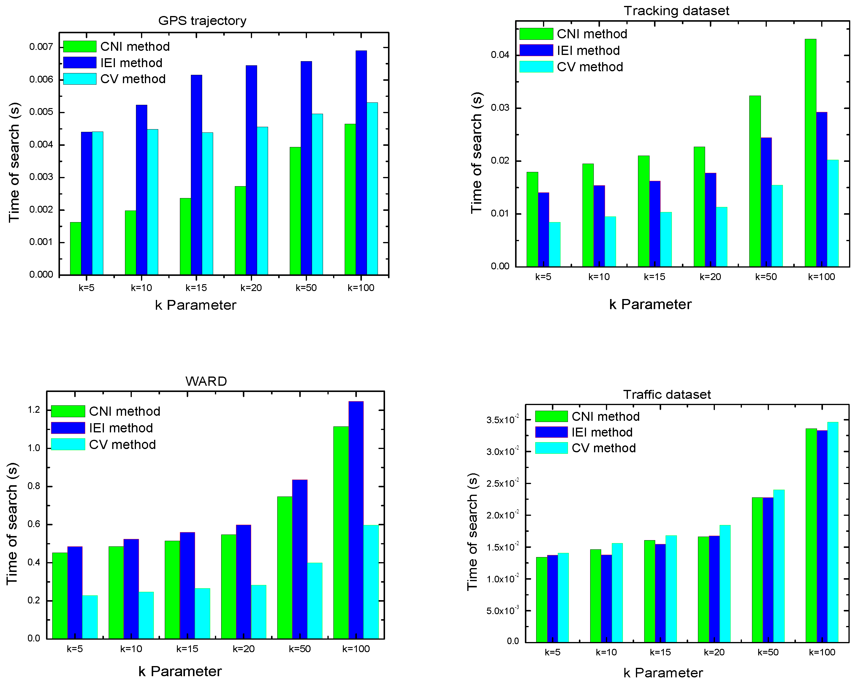
4.5.3. Time of Search

Figure 14 shows the time variation of kNN search queries in BH-trees constructed using the CNI, IEI, and CV methods. The variation in search time was related to the variation in both the average number of distances (Figure 12) and the average number of visited leaves (Figure 15). The shortest time of search for the GPS trajectory dataset was obtained for indexes constructed using the CNI method, where the time of search varied from 0.0016 to 0.0046 s when k varied from 5 to 100. The number of distances and visited leaves was lower for this indexing method than for the other two methods. The time of search in CV-constructed indexes was nearly invariant as a function of k and always fell between those of the CNI and IEI methods. The CV method searched indexes in approximately 0.0048 s. When k varied from 5 to 100, the CV method presented the shortest time for kNN query search, which varied from 0.008 to 0.02 s for the tracking dataset and from 0.227 to 0.596 s for the WARD dataset. Although the IEI method indexes had the shortest search time for the traffic dataset, the search time for the three methods remained close. When k varied from 5 to 100, the search time varied between 0.0137 and 0.0338 s. The time of search for the traffic dataset was less than that for the WARD data because the traffic dataset had fewer visited leaves than the WARD dataset, as shown in Figure 15. For k = 100 and for tracking data, the time of search in indexes by the CV method represented 46 % of that of the CNI method and 69 % of that of the IEI method, while for the WARD data, it represented 53 % and 47 % of that of the CNI and the IEI, respectively.
For the traffic dataset, the time of search in indexes by the IEI method represented 96 % of that of the CV method and the time of search for the CNI method was 97 % of that of the CV method. When the coefficient of variation (CV) of the union of a new cluster from the incoming data stream with the existing first clusters was minimal in the CV method, it indicated that the objects in the two clusters were very similar. Objects from the new cluster were, thus, inserted into the index corresponding to the first cluster, making objects in that index more similar. As a result, the number of distances and visited leaves were lower in the CV method indexes during the kNN query search than in the other methods. Since indexes constructed using CV, CNI, and IEI methods had a constant number of nodes per level, the height of indexes directly influenced the search time for the GPS trajectory dataset (Figure 10).
For k = 100 , the search time in indexes constructed using the CV method was grouped, as evident in in Table 3, with that of other methods for GPS trajectory, tracking dataset and WARD. In the Threshold Distance (TD) method [45], proposed for indexing continuous data streams, the creation of new indexes and the insertion of arrival data in existing indexes was based on a comparison of the distances between cluster centers to a threshold distance value. In this method, the kNN query search proceeded in parallel. The Binary trees, based on Containers at the Cloud-Clusters Fog computing level (B3CF-trees) [39], were constructed in parallel from clusters. These last resulted from the grouping of the whole dataset into clusters of homogeneous objects using the DBSCAN [23] algorithm. In this approach, the kNN query search was combined with parallelism. The Binary tree, based on Containers at the Cloud-Fog computing level (BCCF-tree) [31], was based on the division of the space by means of the k-means [21] clustering algorithm. The BCCF-tree was directly constructed from the whole dataset in the fog layer. The Bubble Buckets tree (BB-tree) [46] recursively partitions the data space into k partitions. The BB-tree leaf nodes stocks objects in elastic buckets named Bubble Buckets. The MX-tree [47] is an enhancement of the M-tree [28], due to the introduction of super-nodes, inspired from the X-tree [48], in the space of the search area. In the Indexing tree Without Containers (IWC-tree), which is a binary tree, simulated from the GH-tree [49], objects are directly inserted without the use of containers. According to Table 3, for the three datasets, the CV method presented the lowest 100NN search time after the B3CF-tree and before the TD method, which reflected its efficiency in indexing continuous data streams. The three indexing methods benefited from the advantages of a combination of parallelism and the kNN search method allowed by the use of the DBSCAN clustering algorithm in the first step of the indexing process. The search time in indexes constructed using the CV method was approximately five times greater than that of the B3CF-tree for the GPS trajectory dataset, and approximately ten times greater for both tracking and WARD datasets. This could be explained by the fact that, in the B3CF-tree, the whole data, which was considered as only one data stream, was grouped into separated clusters of homogeneous objects in each cluster. This allowed the parallel construction of indexes with very similar objects in each one. Compared with the TD method, which also indexes continuous data streams, we can see that the CV method surpassed it in terms of parallel kNN search time. It was approximately 25 times less for the GPS trajectory dataset and twice lower than for both tracking and WARD datasets. The use of the coefficient of variation as the criterion for the homogeneity of the union of clusters induced the construction of BH-trees containing very similar objects. Even if the TD method presented good results, as can be seen in Table 3, its efficiency depended strongly on the choice of the value of the threshold distance. The proposed CV method also proved its efficiency, in terms of search time, compared with other indexing methods, such as that proposed by Zhang et al. [50]. For k = 100 , this team obtained a search time of 0.682 s for a dataset of 1 million size which was, a little greater than our result for the WARD dataset (0.597 s) of 3 millions size.

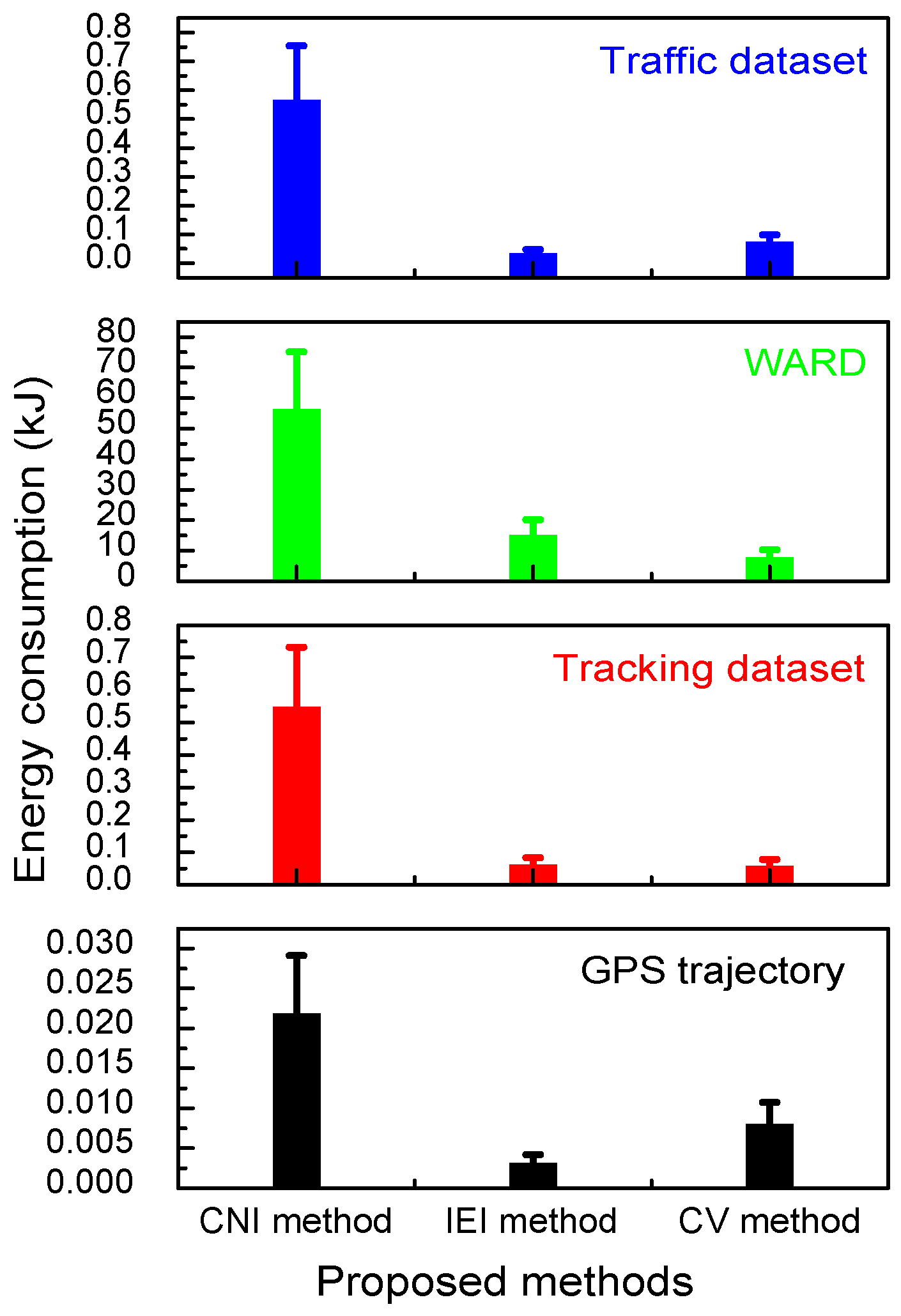
4.5.4. Energy Consumption during the kNN Search

Figure 16 presents the energy consumption during the parallel kNN search with k = 100 in indexes constructed using CV, CNI and IEI methods. For the four datasets chosen, the CNI method consumed more energy than the CV and IEI methods. This was anticipated because using the CNI method results in the creation of more indexes. Furthermore, the use of parallelism causes an increase in energy consumption across all indexes. The energy consumption during the 100NN search in the CV-created indexes was comparable to that of the IEI method, reflecting its efficiency when indexing continuous data streams.
Although the kNN search time in indexes constructed with the CNI and IEI methods was comparable to the above-mentioned methods, some of their characteristics are undesirable for continuous IoT data stream indexing. The CNI method can dynamically index a continuous IoT data stream, resulting in many indexes. The construction of these indices is an expensive process in terms of the numbers of distances and comparisons, computing time, and energy consumption. The cost of the number of distances, the number of comparisons, the time, and energy consumed by search computing during the kNN query search increases as the number of indexes increases. Furthermore, creating a large number of indexes increases the risk of memory overload, which has a negative impact on the indexing process of continuous IoT data. The IEI method indexes the continuous IoT data stream at a low computational cost in terms of distances, comparisons, and time. However, it is not designed to handle continuous IoT data streams. The inclusion of many different elements from the continuous incoming data in a small number of indexes raises their heights and decreases their similarities because the insertion criterion is the shortest distance between the existing and incoming cluster centers. Increasing the depth of indexes, while decreasing their similarities, may result in an increase in the number of distances, comparisons, and times required for kNN search computations. Furthermore, inserting a large number of elements means indexes, constructed using the IEI method, are exposed to the degradation problem.
When compared to the CNI and IEI methods, the CV method was more capable of dynamically indexing the continuous IoT data stream. The coefficient of variation (CV) determines whether the resulting cluster is similar or dissimilar to the existing and incoming clusters. If the union of clusters is similar, incoming elements are inserted into the corresponding existing cluster index, and if not, a new index is built from the incoming cluster. Having similar elements in each index lowers the cost of computing the numbers of distances and comparisons, energy consumption, and kNN query search time. Furthermore, the ability to create new indexes in cases where the union of clusters is not similar, which makes this method suitable for indexing continuous IoT data streams. Using the CV method, the problems of an infinite number of indexes and index degradation are avoided and the construction of new indexes with low-energy consumption and no data overlap is guaranteed.

5. Conclusions

This paper presented the CV method for indexing continuous data streams. The first data stream was clustered using the DBSCAN algorithm at the clustering fog level. The first clusters were stored in the clusters processing fog level, and their corresponding BH-trees were built in the indexing fog level. The incoming cluster either created a new BH-tree or was inserted into an existing BH-tree, depending on the value of the coefficient of variation (CV) of the union of the incoming cluster and the existing clusters. Two other scenarios were proposed for comparison to test the efficiency of our proposed method. In the first scenario, known as the CNI method, each arrival cluster created its own BH-tree.
In the second scenario, known as the IEI method, the objects of the arrival cluster were inserted into an existing BH-tree when the distances between the arrival center cluster and the representative center clusters of the existing indexes were the shortest. In the evaluation of BH-tree construction, the IEI method outperformed the CV and CNI methods. The parameters of the CV method were always located between those of the CNI and IEI methods. The three proposed methods for parallel kNN query search were more efficient than other methods in the literature. In terms of energy consumption, the CV method outperformed the CNI and IEI methods. In future work, we propose to address issues related to geographic and conceptual/domain clustering, as well as to focus on how the effectiveness of the proposed method can be ensured in the movement of data providers from one region to another.

Author Contributions

Conceptualization, K.K., Z.K. and B.F.; methodology, Z.K., H.S. and B.F.; software, K.K., Z.K. and B.F.; validation, K.K., Z.K., M.A.F. and B.F.; investigation, K.K., Z.K., H.S. and B.F.; resources, K.K., Z.K. and B.F.; data curation, K.K., Z.K. and B.F.; writing—original draft preparation, K.K., Z.K., M.A.F. and B.F.; writing—review and editing, K.K., Z.K., M.A.F. and B.F.; visualization, K.K., Z.K., M.A.F. and B.F.; supervision, H.S. and M.A.F.; project administration, H.S., Z.K., and B.F. All authors have read and agreed to the published version of the manuscript.

Funding

This research received no external funding.

Institutional Review Board Statement

Not applicable.

Informed Consent Statement

Not applicable.

Data Availability Statement

Publicly available datasets were analyzed in this study. The GPS trajectory dataset is available in: https://archive.ics.uci.edu/ml/datasets/GPS+Trajectories (accessed on 11 May 2021). The tacking dataset is available in: https://drive.google.com/file/d/1B2Yd2S2b0mLh2tUZjpNNzxrdDrZxvH0b/view?usp=sharing (accessed on 5 April 2021) The WARD dataset is available in: https://people.eecs.berkeley.edu/~yang/software/WAR/ (accessed on 5 December 2021). The traffic dataset is available in: https://networkrepository.com/road.php (accessed on 13 March 2022).

Conflicts of Interest

The authors declare no conflict of interest.

References

  1. Bangui, H.; Ge, M.; Buhnova, B. Exploring Big Data Clustering Algorithms for Internet of Things Applications. In Proceedings of the IoTBDS, Funchal, Portugal, 19–21 March 2018; pp. 269–276. [Google Scholar]
  2. Fathy, Y.; Barnaghi, P.; Tafazolli, R. Large-scale indexing, discovery, and ranking for the Internet of Things (IoT). ACM Comput. Surv. (CSUR) 2018, 51, 1–53. [Google Scholar] [CrossRef]
  3. Demchenko, Y.; Grosso, P.; De Laat, C.; Membrey, P. Addressing big data issues in scientific data infrastructure. In Proceedings of the 2013 International Conference on Collaboration Technologies and Systems (CTS), San Diego, CA, USA, 20–24 May 2013; pp. 48–55. [Google Scholar]
  4. Zhong, Y.; Fang, J.; Zhao, X. VegaIndexer: A distributed composite index scheme for big spatio-temporal sensor data on cloud. In Proceedings of the 2013 IEEE International Geoscience and Remote Sensing Symposium-IGARSS, Melbourne, Australia, 21–26 July 2013; pp. 1713–1716. [Google Scholar]
  5. Zhou, Y.; De, S.; Wang, W.; Moessner, K. Enabling query of frequently updated data from mobile sensing sources. In Proceedings of the 2014 IEEE 17th International Conference on Computational Science and Engineering, Chengdu, China, 19–21 December 2014; pp. 946–952. [Google Scholar]
  6. Gao, X.; Gao, Y.; Zhu, Y.; Chen, G. U 2-Tree: A Universal Two-Layer Distributed Indexing Scheme for Cloud Storage System. IEEE/ACM Trans. Netw. 2019, 27, 201–213. [Google Scholar] [CrossRef]
  7. Mehta, N.; Dang, S. A Review of Clustering Techiques in various Applications for Effective Data Mining. Int. J. Res. IT Manag. 2011, 1, 2231–4334. [Google Scholar]
  8. Makhmutova, A.; Anikin, I. Uncertain Big Data Stream Clustering. In Cyber-Physical Systems; Springer: Berlin/Heidelberg, Germany, 2021; pp. 361–372. [Google Scholar]
  9. Alencar, B.M.; Rios, R.A.; Santana, C.; Prazeres, C. FoT-Stream: A Fog platform for data stream analytics in IoT. Comput. Commun. 2020, 164, 77–87. [Google Scholar] [CrossRef]
  10. Jiang, Y.; Bi, A.; Xia, K.; Xue, J.; Qian, P. Exemplar-based data stream clustering toward Internet of Things. J. Supercomput. 2020, 76, 2929–2957. [Google Scholar] [CrossRef]
  11. Huang, C.Y.; Chang, Y.J. An adaptively multi-attribute index framework for big IoT data. Comput. Geosci. 2021, 155, 104841. [Google Scholar] [CrossRef]
  12. Limkar, S.V.; Jha, R.K. A novel method for parallel indexing of real time geospatial big data generated by IoT devices. Future Gener. Comput. Syst. 2019, 97, 433–452. [Google Scholar] [CrossRef]
  13. Xia, J.; Huang, S.; Zhang, S.; Li, X.; Lyu, J.; Xiu, W.; Tu, W. DAPR-tree: A distributed spatial data indexing scheme with data access patterns to support Digital Earth initiatives. Int. J. Digit. Earth 2020, 13, 1656–1671. [Google Scholar] [CrossRef]
  14. Chaudhry, N.; Yousaf, M.M.; Khan, M.T. Indexing of real time geospatial data by IoT enabled devices: Opportunities, challenges and design considerations. J. Ambient. Intell. Smart Environ. 2020, 12, 281–312. [Google Scholar] [CrossRef]
  15. Chen, L.; Gao, Y.; Song, X.; Li, Z.; Miao, X.; Jensen, C.S. Indexing metric spaces for exact similarity search. arXiv 2020, arXiv:2005.03468. [Google Scholar] [CrossRef]
  16. Zhang, R.; Manotas, I.; Li, M.; Hildebrand, D. Towards a big data benchmarking and demonstration suite for the online social network era with realistic workloads and live data. In Proceedings of the BPOE, Kohala, HI, USA, 31 August–4 September 2015; pp. 25–36. [Google Scholar]
  17. Ma, K.; Bagula, A.; Nyirenda, C.; Ajayi, O. An iot-based fog computing model. Sensors 2019, 19, 2783. [Google Scholar] [CrossRef]
  18. Din, I.U.; Guizani, M.; Hassan, S.; Kim, B.S.; Khan, M.K.; Atiquzzaman, M.; Ahmed, S.H. The Internet of Things: A review of enabled technologies and future challenges. IEEE Access 2018, 7, 7606–7640. [Google Scholar] [CrossRef]
  19. Marjani, M.; Nasaruddin, F.; Gani, A.; Karim, A.; Hashem, I.A.T.; Siddiqa, A.; Yaqoob, I. Big IoT data analytics: Architecture, opportunities, and open research challenges. IEEE Access 2017, 5, 5247–5261. [Google Scholar]
  20. Han, J.; Kamber, M. Data Mining Concepts and Techniques, 2nd ed.; Stephan, A., Ed.; Morgan Kaufmann Publishers Inc.: San Francisco, CA, USA; Elsevier Inc.: San Francisco, CA, USA, 2006; Volume 40, pp. 347–350. [Google Scholar]
  21. Krishna, K.; Murty, M.N. Genetic K-means algorithm. IEEE Trans. Syst. Man Cybern. 1999, 29, 433–439. [Google Scholar] [CrossRef]
  22. Zhang, T.; Ramakrishnan, R.; Livny, M. BIRCH: An efficient data clustering method for very large databases. ACM Sigmod Rec. 1996, 25, 103–114. [Google Scholar] [CrossRef]
  23. Ester, M.; Kriegel, H.P.; Sander, J.; Xu, X. A density-based algorithm for discovering clusters in large spatial databases with noise. In Proceedings of the KDD, Portland, OR, USA, 2–4 August 1996; Volume 96, pp. 226–231. [Google Scholar]
  24. Wang, J.; Wu, S.; Gao, H.; Li, J.; Ooi, B.C. Indexing multi-dimensional data in a cloud system. In Proceedings of the 2010 ACM SIGMOD International Conference on Management of Data, Indianapolis, IN, USA, 6–10 June 2010; pp. 591–602. [Google Scholar]
  25. Wu, S.; Jiang, D.; Ooi, B.C.; Wu, K.L. Efficient B-tree based indexing for cloud data processing. Proc. VLDB Endow. 2010, 3, 1207–1218. [Google Scholar] [CrossRef]
  26. Feng, C.; Yang, X.; Liang, F.; Sun, X.H.; Xu, Z. LCIndex: A local and clustering index on distributed ordered tables for flexible multi-dimensional range queries. In Proceedings of the 2015 44th International Conference on Parallel Processing, Beijing, China, 1–4 September 2015; pp. 719–728. [Google Scholar]
  27. Hong, Y.; Tang, Q.; Gao, X.; Yao, B.; Chen, G.; Tang, S. Efficient R-tree based indexing scheme for server-centric cloud storage system. IEEE Trans. Knowl. Data Eng. 2016, 28, 1503–1517. [Google Scholar] [CrossRef]
  28. Ciaccia, P.; Patella, M.; Zezula, P. M-tree: An efficient access method for similarity search in metric spaces. In Proceedings of the, 23rd International Conference on Very Large Data Bases, Athens, Greece, 25–29 August 1997; Volume 97, pp. 426–435. [Google Scholar]
  29. Kouahla, Z.; Martinez, J. A new intersection tree for content-based image retrieval. In Proceedings of the 2012 10th International Workshop on Content-Based Multimedia Indexing (CBMI), Annecy, France, 27–29 June 2012; pp. 1–6. [Google Scholar]
  30. Kouahla, Z.; Anjum, A.; Akram, S.; Saba, T.; Martinez, J. XM-tree: Data driven computational model by using metric extended nodes with non-overlapping in high-dimensional metric spaces. Comput. Math. Organ. Theory 2019, 25, 196–223. [Google Scholar] [CrossRef]
  31. Benrazek, A.E.; Kouahla, Z.; Farou, B.; Ferrag, M.A.; Seridi, H.; Kurulay, M. An efficient indexing for Internet of Things massive data based on cloud-fog computing. Trans. Emerg. Telecommun. Technol. 2020, 31, e3868. [Google Scholar] [CrossRef]
  32. Khettabi, K.; Kouahla, Z.; Farou, B.; Seridi, H. QCCF-tree: A New Efficient IoT Big Data Indexing Method at the Fog-Cloud Computing Level. In Proceedings of the 2021 IEEE International Smart Cities Conference (ISC2), Manchester, UK, 7–10 September 2021; pp. 1–7. [Google Scholar]
  33. Wang, S.; Maier, D.; Ooi, B.C. Lightweight indexing of observational data in log-structured storage. Proc. VLDB Endow. 2014, 7, 529–540. [Google Scholar] [CrossRef]
  34. Doan, Q.T.; Kayes, A.; Rahayu, W.; Nguyen, K. Integration of iot streaming data with efficient indexing and storage optimization. IEEE Access 2020, 8, 47456–47467. [Google Scholar] [CrossRef]
  35. Ding, Z.; Xu, J.; Yang, Q. SeaCloudDM: A database cluster framework for managing and querying massive heterogeneous sensor sampling data. J. Supercomput. 2013, 66, 1260–1284. [Google Scholar] [CrossRef]
  36. Balakrishna, S.; Thirumaran, M.; Solanki, V.K.; Núñez Valdéz, E.R. Incremental hierarchical clustering driven automatic annotations for unifying IoT streaming data. Int. J. Interact. Multimed. Artif. Intell. 2020, 6, 56–70. [Google Scholar]
  37. Mukherjee, M.; Matam, R.; Shu, L.; Maglaras, L.; Ferrag, M.A.; Choudhury, N.; Kumar, V. Security and privacy in fog computing: Challenges. IEEE Access 2017, 5, 19293–19304. [Google Scholar] [CrossRef]
  38. Al-mamory, S.O.; Algelal, Z.M. A modified DBSCAN clustering algorithm for proactive detection of DDoS attacks. In Proceedings of the 2017 Annual Conference on New Trends in Information & Communications Technology Applications (NTICT), Baghdad, Iraq, 7–9 March 2017; pp. 304–309. [Google Scholar]
  39. Khettabi, K.; Kouahla, Z.; Farou, B.; Seridi, H.; Ferrag, M.A. Clustering and parallel indexing of big IoT data in the fog-cloud computing level. Trans. Emerg. Telecommun. Technol. 2022, 33, e4484. [Google Scholar] [CrossRef]
  40. Liu, T.; Qu, S.; Zhang, K. A Clustering Algorithm for Automatically Determining the Number of Clusters Based on Coefficient of Variation. In Proceedings of the 2nd International Conference on Big Data Research, Weihai, China, 27–29 October 2018; pp. 100–106. [Google Scholar]
  41. Cruz, M.; Macedo, H.T.; Guimarães, A.P. Grouping Similar Trajectories for Carpooling Purposes. In Proceedings of the 2015 Brazilian Conference on Intelligent Systems (BRACIS), Natal, Brazil, 4–7 November 2015; pp. 234–239. [Google Scholar]
  42. Yang, A.Y.; Jafari, R.; Sastry, S.S.; Bajcsy, R. Distributed recognition of human actions using wearable motion sensor networks. J. Ambient. Intell. Smart Environ. 2009, 1, 103–115. [Google Scholar] [CrossRef]
  43. Rossi, R.; Ahmed, N. The network data repository with interactive graph analytics and visualization. In Proceedings of the Twenty-Ninth AAAI Conference on Artificial Intelligence, Austin, TX, USA, 25–30 January 2015. [Google Scholar]
  44. Wu, H.Y.; Lee, C.R. Energy efficient scheduling for heterogeneous fog computing architectures. In Proceedings of the 2018 IEEE 42nd annual computer software and applications conference (COMPSAC), Tokyo, Japan, 23–27 July 2018; Volume 1, pp. 555–560. [Google Scholar]
  45. Khettabi, K.; Kouahla, Z.; Farou, B.; Seridi, H.; Ferrag, M.A. A new method for indexing continuous IoT data flows in metric space. Internet Technol. Lett. 2022, e391. [Google Scholar] [CrossRef]
  46. Sprenger, S.; Schäfer, P.; Leser, U. Bb-tree: A main-memory index structure for multidimensional range queries. In Proceedings of the 2019 IEEE 35th International Conference on Data Engineering (ICDE), Macao, China, 8–11 April 2019; pp. 1566–1569. [Google Scholar]
  47. Jin, S.; Kim, O.; Feng, W. MX-tree: A double hierarchical metric index with overlap reduction. In Proceedings of the Computational Science and Its Applications—ICCSA 2013: 13th International Conference, Ho Chi Minh City, Vietnam, 24–27 June 2013; Springer: Berlin/Heidelberg, Germany, 2013; pp. 574–589. [Google Scholar]
  48. Berchtold, S.; Keim, D.A.; Kriegel, H.P. The X-tree: An index structure for high-dimensional data. In Proceedings of the Very Large Data-Bases, Mumbai, India, 3–6 September 1996; pp. 28–39. [Google Scholar]
  49. Uhlmann, J.K. Satisfying general proximity/similarity queries with metric trees. Inf. Process. Lett. 1991, 40, 175–179. [Google Scholar] [CrossRef]
  50. Zhang, K.; Zhou, W.; Sun, S.; Li, B. Multiple complementary inverted indexing based on multiple metrics. Multimed. Tools Appl. 2019, 78, 7727–7747. [Google Scholar] [CrossRef]
Figure 1. Fog-Cloud computing architecture.
Bdcc 07 00119 g001
Figure 2. Architecture of the CV method.
Bdcc 07 00119 g002
Figure 3. CV method at the cluster processing level.
Bdcc 07 00119 g003
Figure 4. Number of BH-trees vs. data stream.
Bdcc 07 00119 g004
Figure 5. Number of distances calculated during the indexing of each data stream.
Bdcc 07 00119 g005
Figure 6. Number of comparisons calculated during the indexing of each data stream.
Bdcc 07 00119 g006
Figure 7. Indexing time of the data stream using the CV method compared to the IEI and CNI methods.
Bdcc 07 00119 g007
Figure 8. Average energy consumption during index construction using CV, CNI and IEI methods.
Bdcc 07 00119 g008
Figure 9. Average height, average number of internal nodes and average number of leaves nodes of BH-trees constructed using the CV, CNI and IEI methods.
Bdcc 07 00119 g009
Figure 10. Variation of the number of nodes per level of BH-trees constructed using the CNI, IEI and CV methods.
Bdcc 07 00119 g010
Figure 11. Data distribution in leaves.
Bdcc 07 00119 g011
Figure 12. Number of distances calculated for the kNN search in BH-trees by CNI, IEI and CV methods.
Bdcc 07 00119 g012
Figure 13. Number of comparisons calculated for the kNN search in BH-trees by CNI, IEI and CV methods.
Bdcc 07 00119 g013
Figure 14. The kNN search time of CNI, IEI and CV methods.
Bdcc 07 00119 g014
Figure 15. Number of the visited leaves in CNI, IEI and CV methods.
Bdcc 07 00119 g015
Figure 16. Energy consumption during the 100NN search for CNI, IEI and CV methods.
Bdcc 07 00119 g016
Table 1. Table of notations.
AbbreviationExplantation
NNumber of the first clusters
KNumber of the arrival clusters
C l n { n = 1 . . . N } Clusters of the first data stream
Cl k { k = 1 . . . K } Clusters of the arrival data stream
c n { n = 1 . . . N } Cluster centers of the first data stream
c k { k = 1 . . . K } Cluster centers of the arrival data stream
Cl k C l n Union of the arrival clusters Cl k and the first
clusters C l n
d ( c n , c k ) Distance between two centers
I n , { n = 1 . . . N } Set of indexes
M i n d Minimum distances between the centers
of the existing clusters and the incoming clusters
p 1 , p 2 Pivots
ESet of elements
LNLeaf node
INInner node
oObject
LLeft sub tree
RRight sub tree
qQuery
r q Radius for recovering k objects closes to q
AList in with, the set of k objects is stored
B ( q , r q ) Query ball q with radius r q
Table 2. Characteristics of the selected datasets for the index evaluation.
DatasetSize (Vectors)DimensionData Stream Size (Vectors)Data Stream Size (Bytes)
GPS trajectory18,10734000115,507.02
Tracking dataset62,7022012,0001,270,493.8
WARD3,078,5525600,00018,058,184
Traffic dataset5,000,00021,000,00020,132,659.2
Table 3. Comparison of 100NN search time in indexes constructed using the CV method with other methods from literature.
Indexing MethodsCVTD
[45]
B3CF-Tree
[39]
BCCF-Tree
[31]
BB-Tree
[46]
MX-Tree
[47]
IWC-Tree
[31]
Datastes
GPS trajectory0.00531 s0.13583 s0.00118 s0.16191  s0.97994 s0.35414 s0.04013 s
Tracking dataset0.02022 s0.03919 s0.00020 s0.21034  s20.26953 s19.70434 s20.12095 s
WARD0.59673 s1.13473 s0.00576 s2.72482 s116.87681 s3.0745 s120.23918 s
Disclaimer/Publisher’s Note: The statements, opinions and data contained in all publications are solely those of the individual author(s) and contributor(s) and not of MDPI and/or the editor(s). MDPI and/or the editor(s) disclaim responsibility for any injury to people or property resulting from any ideas, methods, instructions or products referred to in the content.

