

A Dual Multimodal Biometric Authentication System Based on WOA-ANN and SSA-DBN Techniques

Abstract
:1. Introduction
- To make an equal combination multimodal biometric framework that utilizes three biometric qualities, specifically ECG, finger impression and sclera.
- To make a successive combination multimodal biometric framework that utilizes three biometric qualities, particularly ECG, unique mark and sclera.
2. Literature Survey
3. Proposed Strategy
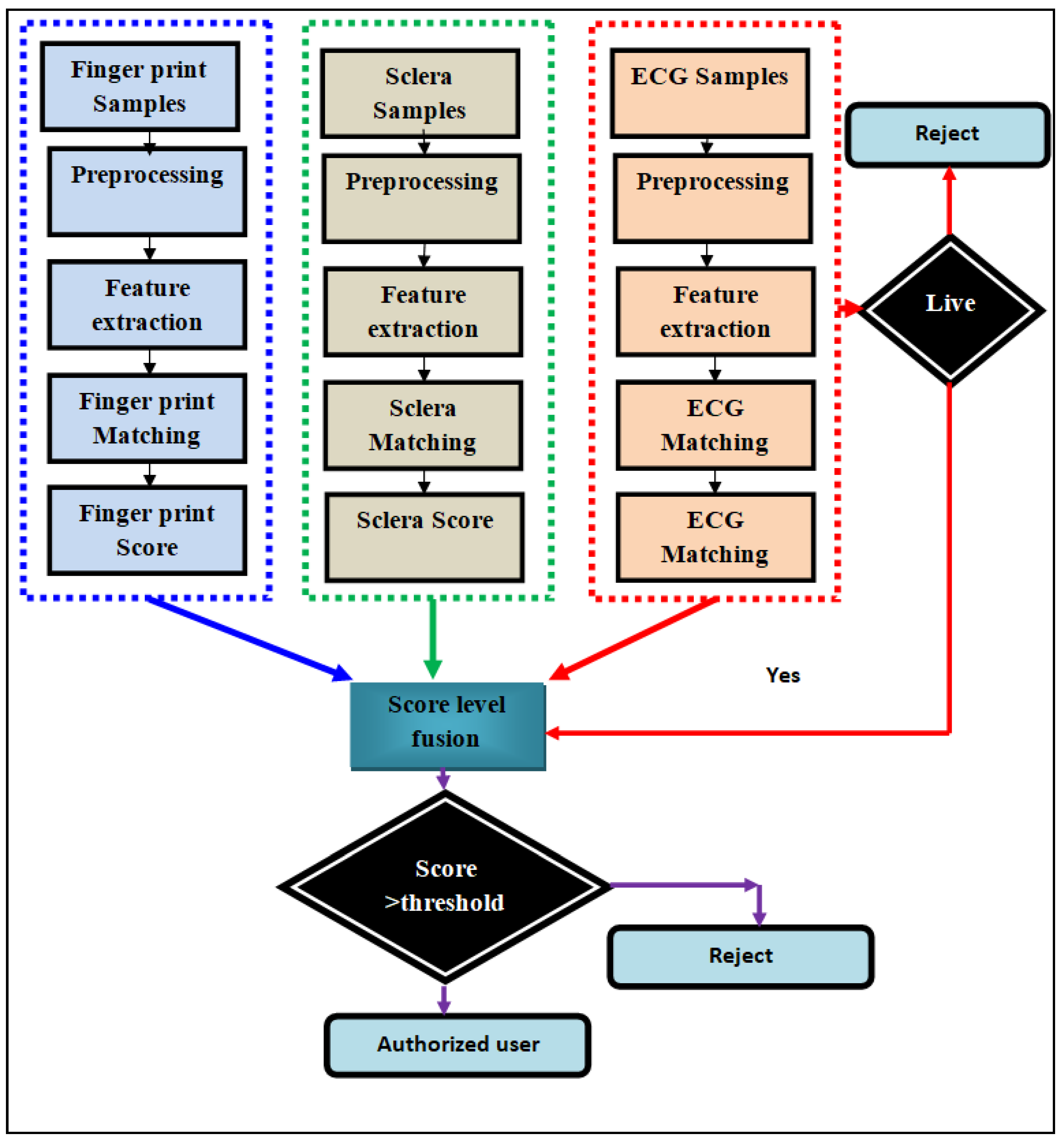
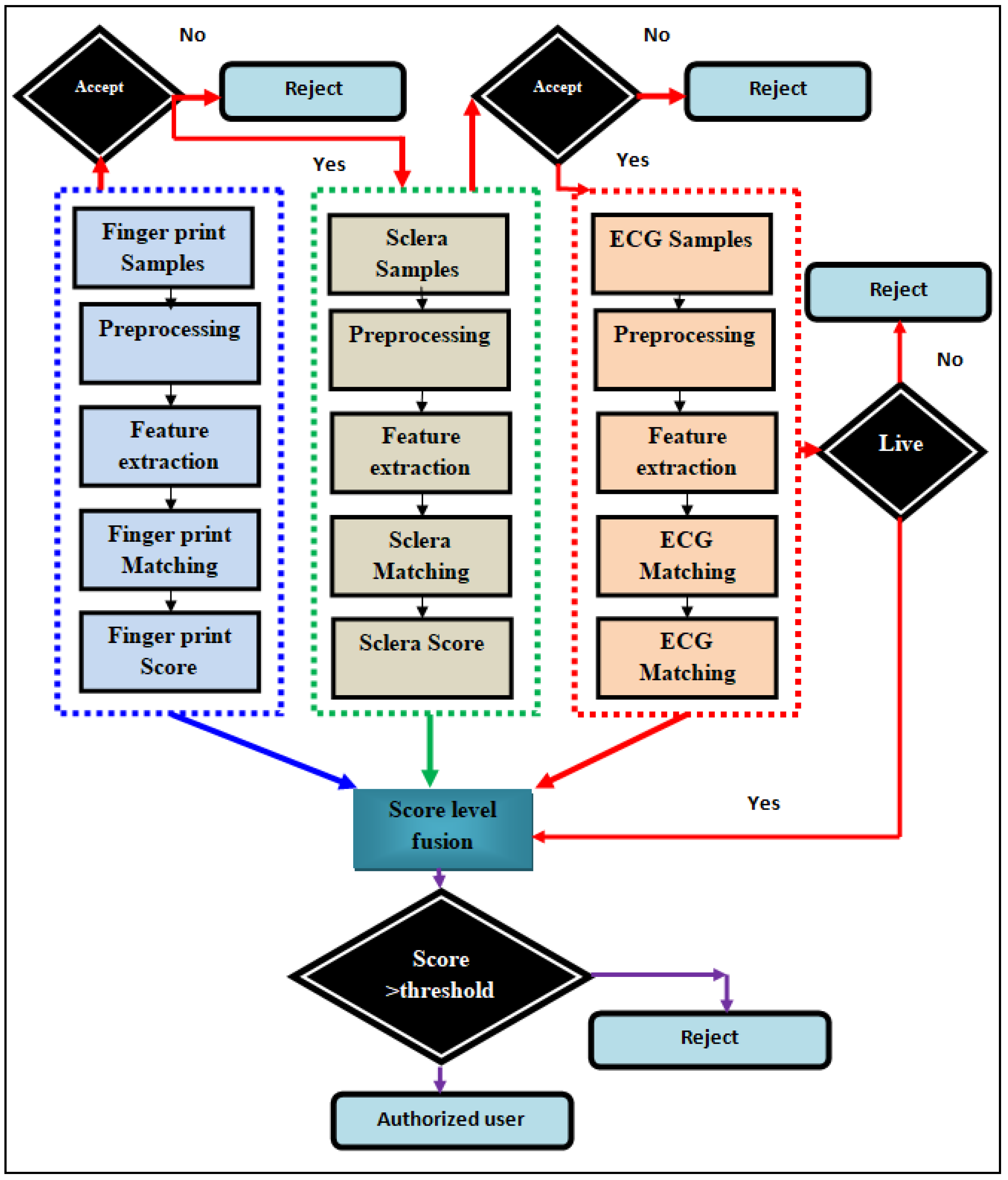
3.1. Parallel and Sequential Modal Common Methodology
3.1.1. Fingerprint
Binarization
Enhancement
- (a)
- Gabor filter
- (b)
- Histrogram Equalization
Feature Extraction
- (a)
- Minutiae Extraction
Normalization
3.1.2. Sclera
Normalization
Bilateral Filter
3.1.3. ECG
Median Filter
QRS Extraction
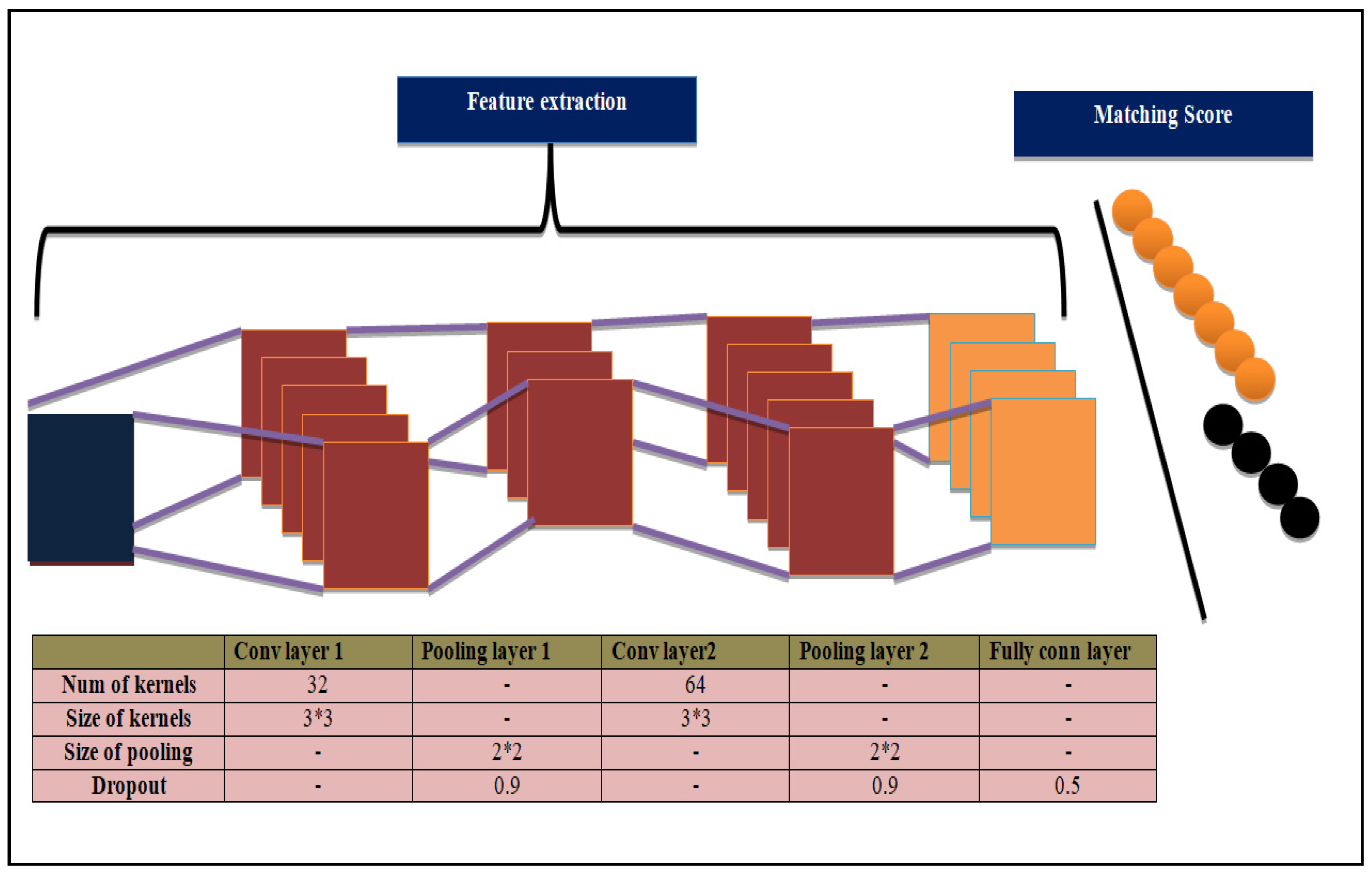
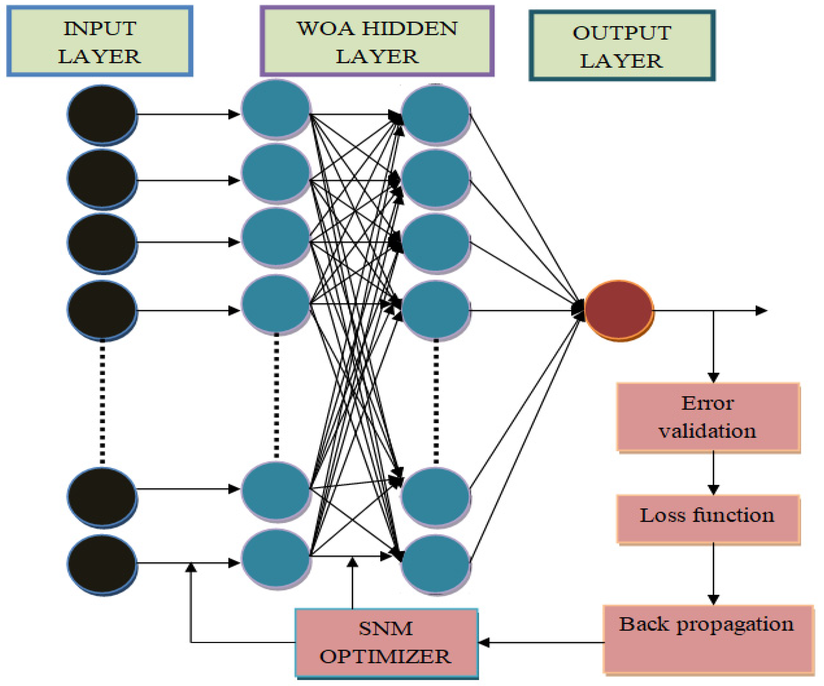
3.1.4. Convolutional Neural Network
Basic Working
3.1.5. Parallel Fusion
3.1.6. Sequential Fusion
4. Results and Discussion
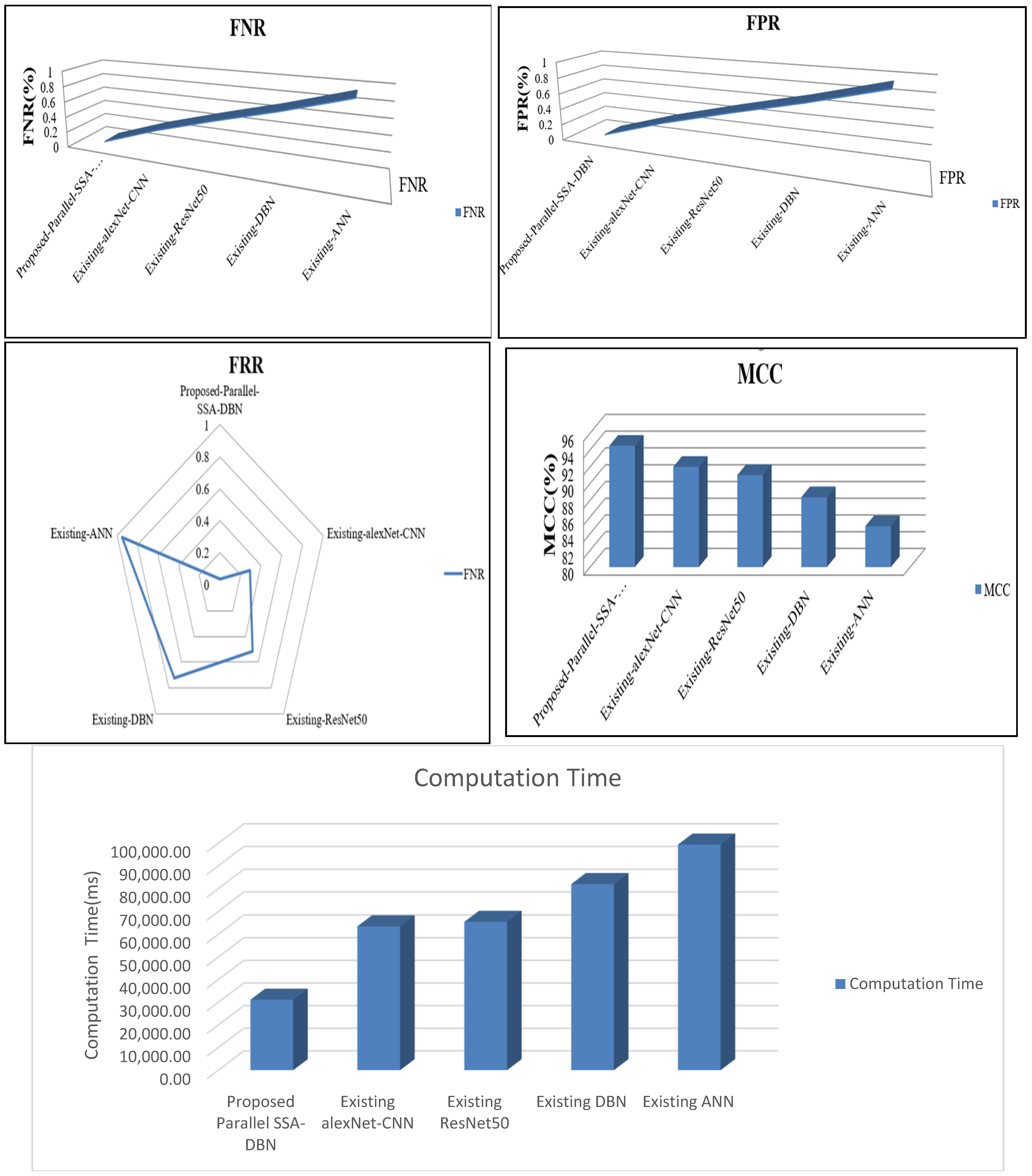
4.1. Performance Analysis of Parallel Modal Architecture
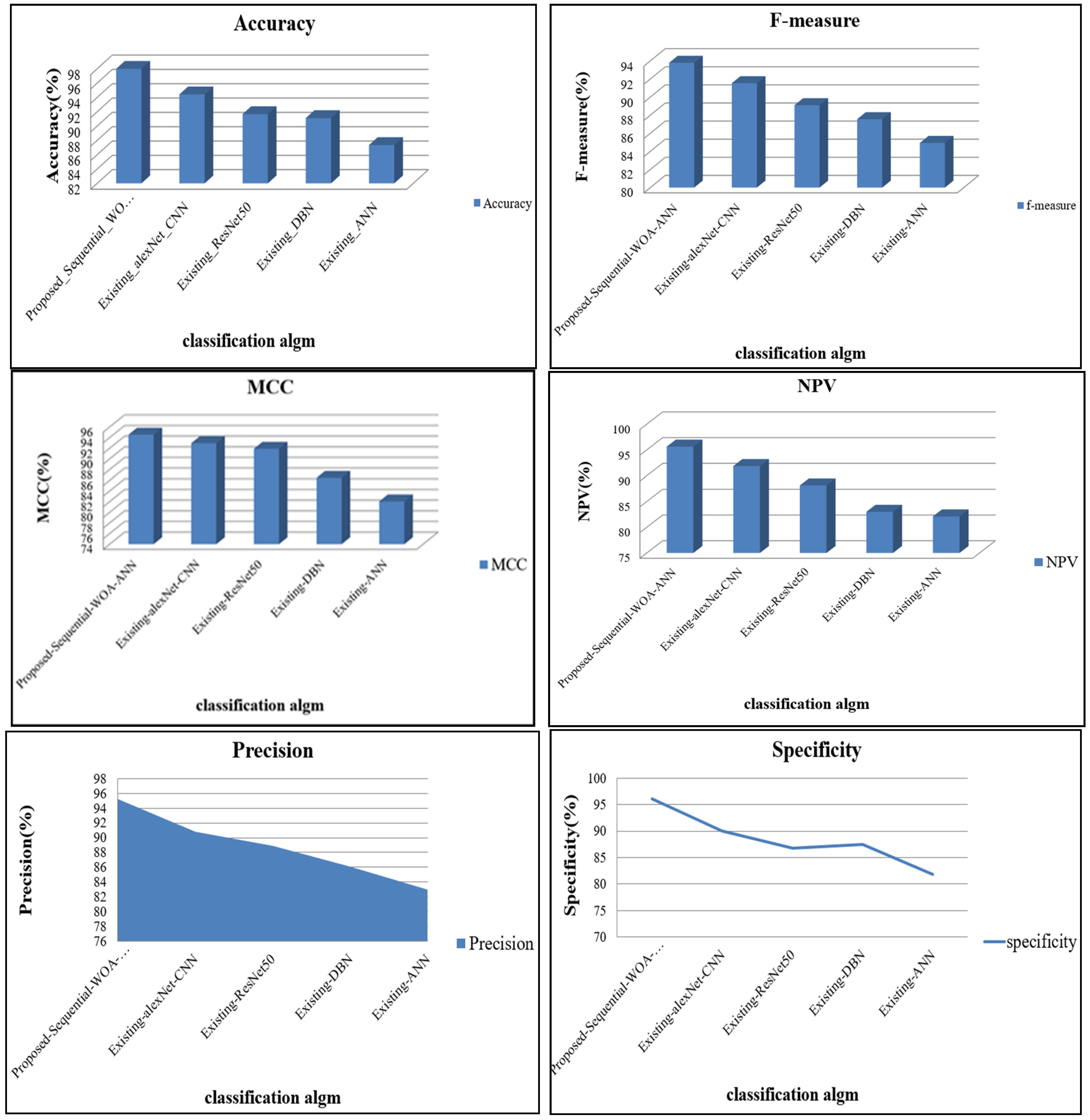
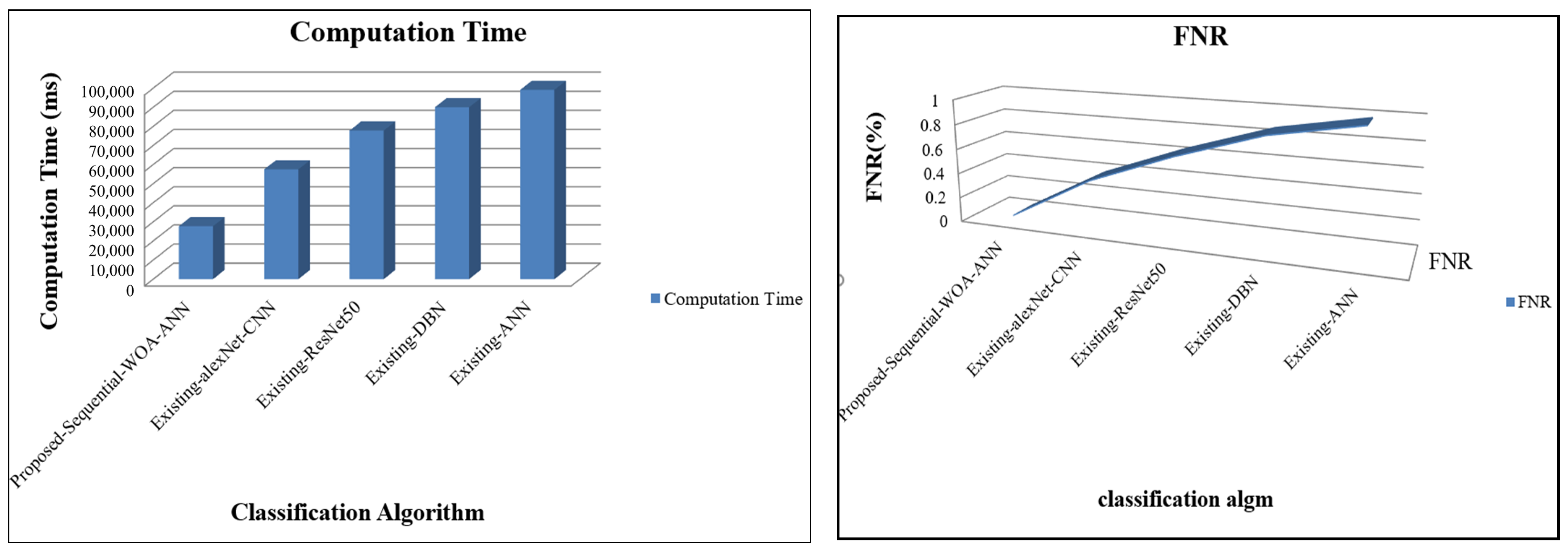
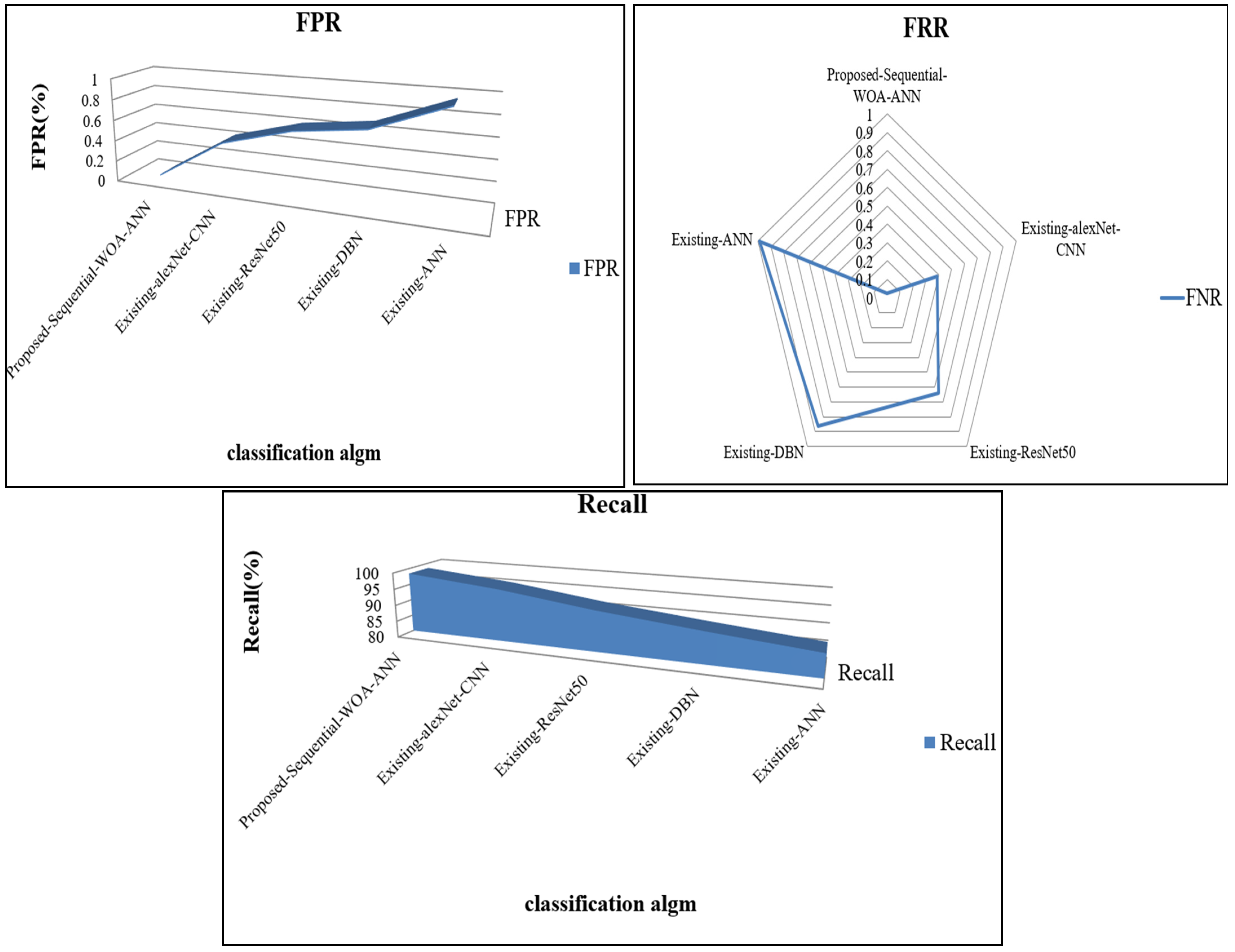
4.2. Performance Analysis of Proposed Sequential Modal Architecture
5. Conclusions
Author Contributions
Funding
Data Availability Statement
Conflicts of Interest
References
- Sudhamani, M.J.; Sanyal, I.; Venkatesha, M.K. Artificial Neural Network Approach for multimodal biometric authentication system. In Proceedings of Data Analytics and Management; Springer: Singapore, 2021; pp. 253–265. [Google Scholar]
- Balaji, S.; Rahamathunnisa, U. A Review on Multimodal Biometric Authentication in Healthcare. In Proceedings of the 8th International Conference on Advanced Computing and Communication Systems, Coimbatore, India, 25–26 March 2022; Volume 1, pp. 1–5. [Google Scholar]
- Bala, N.; Gupta, R.; Kumar, A. Multimodal Biometric System Based on Fusion Techniques: A Review. Inf. Secur. J. A Glob. Perspect. 2022, 31, 289–337. [Google Scholar] [CrossRef]
- Gayathri, M.; Malathy, C.; Prabhakaran, M. A Review on Various Biometric Techniques, Its Features, Methods, Security Issues and Application Areas. In Computational Vision and Bio-Inspired Computing; Springer: Cham, Switzerland, 2020; pp. 931–941. [Google Scholar]
- Shalini, P. Multimodal biometric decision fusion security technique to evade immoral social networking sites for minors. Appl. Intell. 2023, 53, 2751–2776. [Google Scholar] [CrossRef]
- Ahamed, F.; Farid, F.; Suleiman, B.; Jan, Z.; Wahsheh, L.A.; Shahrestani, S. An Intelligent Multimodal Biometric Authentication Model for Personalised Healthcare Services. Future Internet 2022, 14, 222. [Google Scholar] [CrossRef]
- Ketab, S.S.; Clarke, N.L.; Dowland, P.S. A Robust E-Invigilation System Employing Multimodal Biometric Authentication. Int. J. Inf. Educ. Technol. 2017, 7, 796–802. [Google Scholar] [CrossRef] [Green Version]
- Kandasamy, M. Multimodal Biometric Crypto System for Human Authentication Using Ear and Palm Print. Pattern Anal. Appl. 2022, 25, 1015–1024. [Google Scholar] [CrossRef]
- Thenuwara, S.S.; Premachandra, C.; Kawanaka, H. A Multi-Agent Based Enhancement for Multimodal Biometric System at Border Control. Array 2022, 14, 100171. [Google Scholar] [CrossRef]
- Vensila, C.; Wesley, A.B. Multimodal Biometric Authentication Using Watermarking Technique. In Security, Privacy and Data Analytics; Springer: Singapore, 2022; pp. 79–91. [Google Scholar]
- Elavarasi, G.; Vanitha, M. Multimodal Biometric Authentication by Slap Swarm-Based Score Level Fusion. In Proceedings of Data Analytics and Management; Springer: Singapore, 2021; pp. 831–842. [Google Scholar]
- Ren, H.; Sun, L.; Guo, J.; Han, C. A Dataset and Benchmark for Multimodal Biometric Recognition Based on Fingerprint and Finger Vein. IEEE Trans. Inf. Forensics Secur. 2022, 17, 2030–2043. [Google Scholar] [CrossRef]
- Channegowda, A.B.; Prakash, H.N. Image Fusion by Discrete Wavelet Transform for Multimodal Biometric Recognition. IAES Int. J. Artif. Intell. (IJ-AI) 2022, 11, 229. [Google Scholar] [CrossRef]
- Tyagi, S.; Chawla, B.; Jain, R.; Srivastava, S. Multimodal biometric system using deep learning based on face and finger vein fusion. J. Intell. Fuzzy Syst. 2022, 42, 943–955. [Google Scholar] [CrossRef]
- Sarangi, P.P.; Nayak, D.R.; Panda, M.; Majhi, B. A feature-level fusion based improved multimodal biometric recognition system using ear and profile face. J. Ambient. Intell. Humaniz. Comput. 2022, 13, 1867–1898. [Google Scholar] [CrossRef]
- Medjahed, C.; Rahmoun, A.; Charrier, C.; Mezzoudj, F. A deep learning-based multimodal biometric system using score fusion. IAES Int. J. Artif. Intell. 2022, 11, 65. [Google Scholar] [CrossRef]
- Heidari, H.; Chalechale, A. Biometric Authentication Using a Deep Learning Approach Based on Different Level Fusion of Finger Knuckle Print and Fingernail. Expert Syst. Appl. 2022, 191, 116278. [Google Scholar] [CrossRef]
- El-Rahiem, B.A.; El-Samie, F.E.A.; Amin, M. Multimodal Biometric Authentication Based on Deep Fusion of Electrocardiogram (ECG) and Finger Vein. Multimed. Syst. 2022, 28, 1325–1337. [Google Scholar] [CrossRef]
- Valsaraj, A.; Madala, I.; Garg, N.; Patil, M.; Baths, V. Motor Imagery Based Multimodal Biometric User Authentication System Using EEG. In Proceedings of the International Conference on Cyberworlds (CW), Caen, France, 29 September–1 October 2020; pp. 272–279. [Google Scholar]
- Cherifi, F.; Amroun, K.; Omar, M. Robust Multimodal Biometric Authentication on IoT Device through Ear Shape and Arm Gesture. Multimed. Tools Appl. 2021, 80, 14807–14827. [Google Scholar] [CrossRef]
- Gavisiddappa, G.; Mahadevappa, S.; Patil, C. Multimodal Biometric Authentication System Using Modified ReliefF Feature Selection and Multi Support Vector Machine. Int. J. Intell. Eng. Syst. 2020, 13, 1–12. [Google Scholar] [CrossRef]
- Vitek, M.; Rot, P.; Štruc, V.; Peer, P. A Comprehensive Investigation into Sclera Biometrics: A Novel Dataset and Performance Study. Neural Comput. Appl. 2020, 32, 17941–17955. [Google Scholar] [CrossRef]
- Goldberger, A.L.; Amaral, L.A.N.; Glass, L.; Hausdorff, J.M.; Ivanov, P.C.; Mark, R.G.; Mietus, J.E.; Moody, G.B.; Peng, C.-K.; Stanley, H.E. PhysioBank, PhysioToolkit, and PhysioNet: Components of a new research resource for complex physiologic signals. Circulation 2000, 101, 215–220. [Google Scholar] [CrossRef] [PubMed] [Green Version]
- Liu, H.; Liu, T.; Zhang, Z.; Sangaiah, A.K.; Yang, B.; Li, Y. ARHPE: Asymmetric Relation-Aware Representation Learning for Head Pose Estimation in Industrial Human–Computer Interaction. IEEE Trans. Ind. Inform. 2022, 18, 7107–7117. [Google Scholar] [CrossRef]
- Liu, H.; Liu, T.; Chen, Y.; Zhang, Z.; Li, Y.-F. EHPE: Skeleton Cues-Based Gaussian Coordinate Encoding for Efficient Human Pose Estimation. IEEE Trans. Multimed. 2022, 1–12. [Google Scholar] [CrossRef]
- Liu, H.; Fang, S.; Zhang, Z.; Li, D.; Lin, K.; Wang, J. MFDNet: Collaborative Poses Perception and Matrix Fisher Distribution for Head Pose Estimation. IEEE Trans. Multimed. 2021, 24, 2449–2460. [Google Scholar] [CrossRef]


| Techniques | Recall | f-Measure | NPV | Specificity | Accuracy | Precision |
|---|---|---|---|---|---|---|
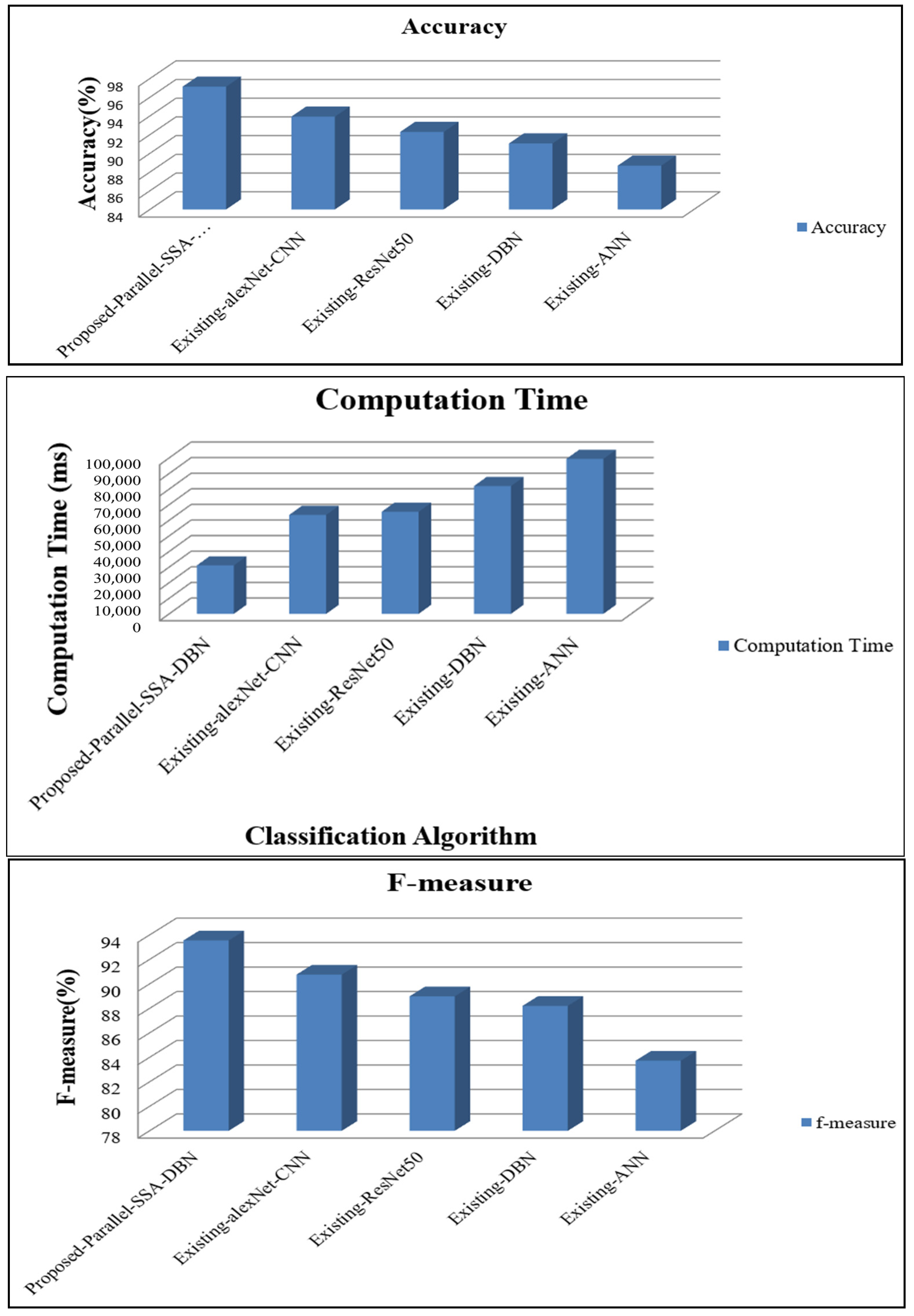
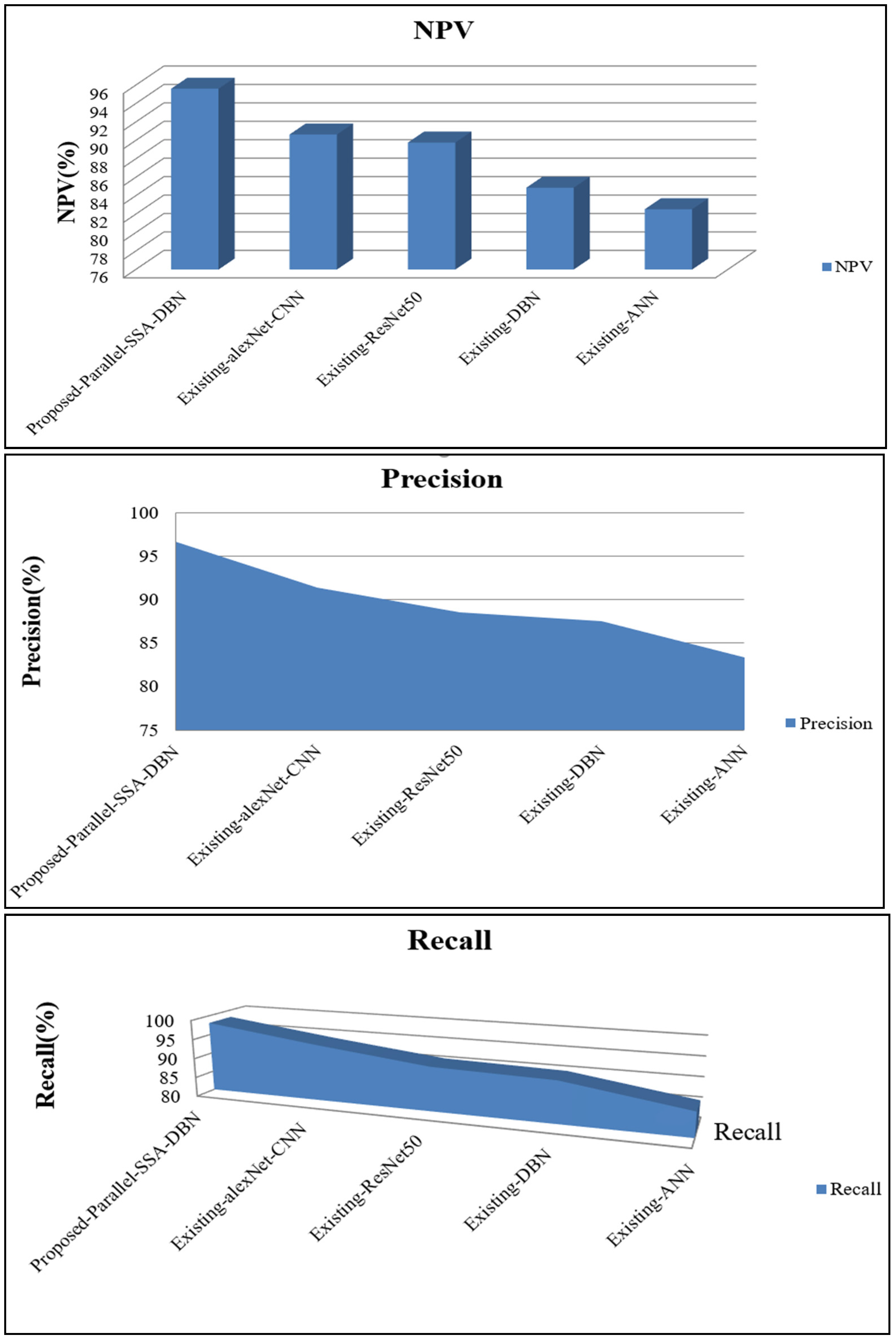
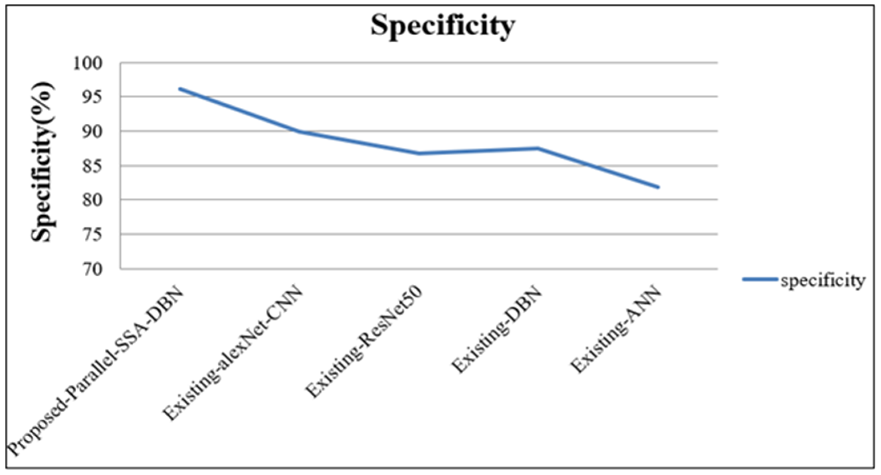
| Proposed Parallel SSA-DBN | 98.12 | 93.55 | 95.62 | 96.11 | 97.13 | 96.65 |
| Existing alexNet-CNN | 94.44 | 90.76 | 90.65 | 90.00 | 93.93 | 91.38 |
| Existing ResNet50 | 91.22 | 88.99 | 89.78 | 86.74 | 92.29 | 88.57 |
| Existing DBN | 90.52 | 88.21 | 84.88 | 87.45 | 91.06 | 87.55 |
| Existing ANN | 86.12 | 83.73 | 82.54 | 81.86 | 88.69 | 83.38 |
| Techniques | FPR | MCC | FRR | Computation Time | FNR |
|---|---|---|---|---|---|
| Proposed Parallel SSA-DBN | 0.02 | 94.49 | 0.03 | 31,117.00 | 0.03 |
| Existing alexNet-CNN | 0.37 | 92.00 | 0.29 | 63,474.00 | 0.29 |
| Existing ResNet50 | 0.53 | 91.00 | 0.51 | 65,454.00 | 0.51 |
| Existing DBN | 0.61 | 88.37 | 0.72 | 81,986.00 | 0.72 |
| Existing ANN | 0.96 | 84.89 | 0.95 | 99,384.00 | 0.95 |
| Specificity | Accuracy | Precision | F-Measure | NPV | MCC | |
|---|---|---|---|---|---|---|
| Proposed Sequential WOA-ANN | 95.54 | 98.00 | 95.23 | 93.79 | 95.63 | 94.56 |
| Existing alexNet-CNN | 91.46 | 94.42 | 90.85 | 91.54 | 91.85 | 92.95 |
| Existing ResNet50 | 87.00 | 91.67 | 88.86 | 89.10 | 88.13 | 91.89 |
| Existing DBN | 87.69 | 91.12 | 86.11 | 87.56 | 83.00 | 86.46 |
| Existing ANN | 80.18 | 87.35 | 82.94 | 84.93 | 82.11 | 82.05 |
| FPR | FRR | Computation Time (ms) | FNR | Recall | |
|---|---|---|---|---|---|
| Proposed Sequential WOA-ANN | 0.0311 | 0.024 | 27,717 | 0.02 | 98.46 |
| Existing alexNet-CNN | 0.4295 | 0.388 | 57,464 | 0.39 | 95.90 |
| Existing ResNet50 | 0.6112 | 0.644 | 77,814 | 0.64 | 92.22 |
| Existing DBN | 0.6966 | 0.861 | 89,986 | 0.86 | 89.35 |
| Existing ANN | 0.9572 | 0.986 | 99,114 | 0.99 | 86.74 |
Disclaimer/Publisher’s Note: The statements, opinions and data contained in all publications are solely those of the individual author(s) and contributor(s) and not of MDPI and/or the editor(s). MDPI and/or the editor(s) disclaim responsibility for any injury to people or property resulting from any ideas, methods, instructions or products referred to in the content. |
© 2023 by the authors. Licensee MDPI, Basel, Switzerland. This article is an open access article distributed under the terms and conditions of the Creative Commons Attribution (CC BY) license (https://creativecommons.org/licenses/by/4.0/).
Share and Cite
Singh, S.P.; Tiwari, S. A Dual Multimodal Biometric Authentication System Based on WOA-ANN and SSA-DBN Techniques. Sci 2023, 5, 10. https://doi.org/10.3390/sci5010010
Singh SP, Tiwari S. A Dual Multimodal Biometric Authentication System Based on WOA-ANN and SSA-DBN Techniques. Sci. 2023; 5(1):10. https://doi.org/10.3390/sci5010010
Chicago/Turabian StyleSingh, Sandeep Pratap, and Shamik Tiwari. 2023. "A Dual Multimodal Biometric Authentication System Based on WOA-ANN and SSA-DBN Techniques" Sci 5, no. 1: 10. https://doi.org/10.3390/sci5010010