A Concise Tutorial on Functional Analysis for Applications to Signal Processing

Abstract

Functional analysis is a well-developed field in the discipline of Mathematics, which provides unifying frameworks for solving many problems in applied sciences and engineering. In particular, several important topics (e.g., spectrum estimation, linear prediction, and wavelet analysis) in signal processing had been initiated and developed through collaborative efforts of engineers and mathematicians who used results from Hilbert spaces, Hardy spaces, weak topology, and other topics of functional analysis to establish essential analytical structures for many subfields in signal processing. This paper presents a concise tutorial for understanding the theoretical concepts of the essential elements in functional analysis, which form a mathematical framework and backbone for central topics in signal processing, specifically statistical and adaptive signal processing. The applications of these concepts for formulating and analyzing signal processing problems may often be difficult for researchers in applied sciences and engineering, who are not adequately familiar with the terminology and concepts of functional analysis. Moreover, these concepts are not often explained in sufficient details in the signal processing literature; on the other hand, they are well-studied in textbooks on functional analysis, yet without emphasizing the perspectives of signal processing applications. Therefore, the process of assimilating the ensemble of pertinent information on functional analysis and explaining their relevance to signal processing applications should have significant importance and utility to the professional communities of applied sciences and engineering. The information, presented in this paper, is intended to provide an adequate mathematical background with a unifying concept for apparently diverse topics in signal processing. The main objectives of this paper from the above perspectives are summarized below: (1) Assimilation of the essential information from different sources of functional analysis literature, which are relevant to developing the theory and applications of signal processing. (2) Description of the underlying concepts in a way that is accessible to non-specialists in functional analysis (e.g., those with bachelor-level or first-year graduate-level training in signal processing and mathematics). (3) Signal-processing-based interpretation of functional-analytic concepts and their concise presentation in a tutorial format.

1. Introduction

The concept of functional analysis is built upon normed vector spaces and particularly inner product spaces, which are merged with diverse notions of topology and geometry, linear algebra, probability theory, and real and complex analysis (see, e.g., [1,2,3,4,5]). Topics in functional analysis include various concepts such as Banach spaces and Hilbert spaces, and linear operators and their spectral theory, as well as group and semigroup theory. Knowledge of these mathematical structures is often essential for understanding and solving a variety of analytical problems in signal processing and related fields, as well as in mathematics itself [5]. For example, in functional analysis, objects like functions are considered as elements or points in a space of functions [6], and hence the name functional analysis.

Results, generated from functional analysis, form key concepts in the frameworks of advanced scientific and engineering disciplines that include the fields of statistical signal processing and adaptive signal processing. Although adaptive signal processing can be viewed as a branch of statistical signal processing [7], the special properties of this field and their roles in engineering applications have led many specialists to consider them as two separate fields. Therefore, in many universities and research institutions around the world, statistical signal processing and adaptive signal processing are taught as independent graduate courses in engineering and applied sciences, and many textbooks have been devoted to study these important fields individually (e.g., see [8,9] and references therein). Nevertheless both statistical signal processing and adaptive signal processing form the backbone of the so-called modern signal processing, in which signals are generally considered as random processes. Modern signal processing covers many topics of current interest, such as signal modeling and estimation, signal prediction, signal compression, adaptive lattice filtering, adaptive joint process estimation, recursive least squares lattice filtering, and spectrum estimation. The issues, related to processing of both deterministic and random signals, are further discussed below.

While an estimation error may typically converge to zero for deterministic signals, this is generally not the case for random signals [8]. Therefore, in statistical and adaptive signal processing, it is a common practice for random signals to make them unbiased (i.e., expectation of the estimation error converging to zero). As explained later, this type of convergence is of a special kind, which is known in functional analysis as weak convergence (see, for example, [10,11]). Therefore, many important results in functional analysis are obtained in terms of weak convergence and weak topology, which potentially have significant implications to the subfields of statistical signal processing and adaptive signal processing. Moreover, it is usually desirable in estimation theory to identify optimal filters, which bridges the discipline of signal processing to that of optimization theory. To this end, researchers in modern signal processing often deal with random processes for which optimization problems become more challenging, and the usage of advanced mathematical tools is justified.

From a historical perspective, the names of some of the spaces used in functional analysis are those of early-time mathematicians who had originally developed the theories of these spaces. Indeed much of the theoretical work has been associated with the names of eminent mathematicians (e.g., Gauss, Lagrange, Euler, and Kolmogorov). In fact, the Hilbert space, which is a central topic in functional analysis, is one of the most commonly used mathematical frameworks of signal processing and the associated optimization [12]. The unique features of Hilbert spaces are explained in the paper from these perspectives. However, the names of other well-known spaces (e.g., metric spaces and normed spaces) were given based on the technical properties of these spaces; many of the spaces, frequently used in functional analysis, have been named based on quite different historical backgrounds.

We have presented a concise and focused review of key concepts of functional analysis in this paper, which have strong relevance to modern signal processing. The most important spaces from the perspectives of functional analysis, considered in this paper, are metric/topological spaces, Banach spaces, and Hilbert spaces. The relations among these and other spaces are illustrated in Figure 1. Other relevant vector spaces like summable (${\ell }^p$), Lebesgue-integrable ($L^p$), and Hardy (${\mathcal{H}}^p$) spaces are also introduced in the paper.

The paper is organized in four sections, including the current section, and an Appendix A. Section 2 introduces Banach spaces and their relevant theorems, where special emphases are laid on the ${\ell }^p$/$L^p$ spaces, ${\mathcal{H}}^p$ spaces, spectral factorization, and weak topology in the setting of Banach spaces. Section 3 presents Hilbert spaces and their relevant features (e.g., Fourier series expansion and the orthogonality principle) along with some applications to signal processing and detection theory, such as wavelets, Karhunen-Loéve (KL) expansion, and reproducing-kernel Hilbert spaces (RKHS). Section 4 summarizes and concludes the paper. The Appendix A in this paper introduces elementary concepts and definitions in real analysis, probability theory, and topological spaces, which should be helpful for understanding the fundamental principles of functional analysis as applied to various concepts of signal processing; however the readers, who are familiar with these concepts, may only selectively refer to the Appendix A.

2. Banach Spaces for Signal Analysis

This section deals with Banach spaces for general applications to signal processing; it also introduces the concepts of Hardy spaces especially for digital signal processing. Further details on Banach spaces are provided in standard books on functional analysis such as Bachman and Narici [1] and Naylor and Sell [2].

2.1. Introduction to Banach Spaces

We start this subsection with the definition of a Banach space which is a complete normed space as defined below.

Definition 1

(Banach Spaces). Let a vector space X be defined over a field $\mathbb{K}$, where examples of $\mathbb{K}$ are the field of real numbers $(\mathbb{R},+,·)$ and the field of complex numbers $(\mathbb{C},+,·)$. Let a function $\parallel •\parallel :X\to \mathbb{R}$, called norm and denoted as $x\mapsto \parallel x\parallel$, have the following properties:

• (positivity) $\forall x\in X,\parallel x\parallel \ge 0,\forall x\in X$, and $\parallel x\parallel =0$ if and only if $x=0$.
• (homogeneity) $\forall x\in X$ and $\forall c\in \mathbb{K},\parallel cx\parallel =\left|c\right|\parallel x\parallel$.
• (triangular inequality) $\forall x,y\in X,\parallel x+y\parallel \le \parallel x\parallel +\parallel y\parallel$.

Then, $\left(X,\parallel •\parallel \right)$ is called a normed vector space, where the norm $\parallel •\parallel$ serves as a metric. A real (resp. complex) normed linear space that is complete (i.e., where every Cauchy sequence converges in the space) is called a real (resp. complex) Banach space.

Example 1.

The spaces of ${\ell }^p$ sequences, $1\le p\le \infty$, form an important class of Banach spaces, which are extensively used in digital signal processing. These are linear vector spaces of all real (resp. complex) sequences $x\triangleq \{x_n\}$ such that ${\sum }_{n=-\infty }^{\infty }{\left|x_n\right|}^p<\infty$, where the ${\ell }^p$-norm is defined as:

$${\parallel x\parallel }_{{\ell }^p}\triangleq {\left(\sum _{n=-\infty }^{\infty }{\left|x_n\right|}^p\right)}^{1/p}\mathit{if}1\le p<\infty$$

$${\parallel x\parallel }_{{\ell }^{\infty }}\triangleq \underset{n\in \mathbb{Z}}{sup}\left|x_n\right|\mathit{if}p=\infty$$

Some of the theorems on ${\ell }^p$ spaces [2], which are extensively used in the analyses of discrete-time signals, are presented below.

Theorem 1

(Hölder Inequality [2]). Let $1<p<\infty$ and $\frac{1}{p}+\frac{1}{q}=1$. If $f\in {\ell }^p$ and $g\in {\ell }^q$, then $f·g\in {\ell }^1$ and ${\parallel f·g\parallel }_{{\ell }^1}\le {\parallel f\parallel }_{{\ell }^p}{\parallel g\parallel }_{l^q}$.

Proof. 

See pp. 550–551 in Naylor and Sell [2]. □

It is noted that Hölder Inequality also holds for $p=1$ and $p=\infty$.

Theorem 2

(Minkowski inequality [2]). If $1\le p\le \infty$ and $f,g\in {\ell }^p$, then ${\parallel f+g\parallel }_{{\ell }^p}\le {\parallel f\parallel }_{{\ell }^p}+{\parallel g\parallel }_{{\ell }^p}$.

Proof. 

See pp. 550–551 in Naylor and Sell [2]. □

It is noted that Lebesgue-integrable versions of ${\ell }^p$ spaces, for applications to continuous signal processing, are called $L^p$ spaces [4]. In $L^p$ spaces, Hölder inequality and Minkowski inequality are similar to their respective ${\ell }^p$-versions in Theorems 1 and 2.

Next we focus on a few systems-theoretic applications of Banach spaces, which would require the operation of convolution.

Theorem 3

(Convolution inequality [13]). For the sequences $\mathbf{u}\in {\ell }^p$ for $p\in [1,\infty ]$ and $\mathbf{h}\in {\ell }^1$, the convolution product $\mathbf{h}\ast \mathbf{u}\in {\ell }^p$ and ${\parallel \mathbf{h}\ast \mathbf{u}\parallel }_{{\ell }^p}\le {\parallel \mathbf{h}\parallel }_{{\ell }^1}{\parallel \mathbf{u}\parallel }_{{\ell }^p}$.

Proof. 

See p. 241 in Desoer and Vidyasagar [13]. □

Lemma 1

(Barbalat Lemma). If $\{x_n\}\in l^p$ for some $p\in [1,\infty )$, then ${lim}_{n\to \infty }\left|x_n\right|=0$.

Proof. 

Let us assume that ${lim}_{n\to \infty }\left|x_n\right|\ne 0$ is true. Then, there exists a subsequence $\{|x_{n_j}|\}$ bounded below by a real number $\epsilon >0$, which implies that $\{|x_{n_j}{|}^p\}$ is bounded below by ${\epsilon }^p$ so that ${\sum }_n{\left|x_n\right|}^p\to \infty$ as $n\to \infty$. This contradicts the assertion $\{x_n\}\in {\ell }^p$. □

Let a linear discrete-time dynamical system with an impulse response $\mathbf{h}[n,k]$ be excited by an input signal $\mathbf{u}$ to yield an output signal $\mathbf{y}$.

Definition 2

(BIBO-stability). A system is said to be bounded-input-bounded-output (BIBO)-stable if every $\mathbf{u}\in {\ell }^{\infty }\Rightarrow \mathbf{y}\in {\ell }^{\infty }$. More generally, the system is called ${\ell }^p$-stable if $\mathbf{u}\in {\ell }^p\Rightarrow \mathbf{y}\in {\ell }^p$, where $p\in [1,\infty ]$.

For a linear shift-invariant (LSI) system, the impulse response $\mathbf{h}[n,k]$ takes the form $\mathbf{h}[n-k]$, where the output is given by the convolution $\mathbf{y}=\mathbf{h}\star \mathbf{u}$ as [14]:

$$\mathbf{y}\left[n\right]=\sum _{k=-\infty }^{\infty }\mathbf{h}[n-k]\mathbf{u}\left[k\right]=\sum _{k=-\infty }^{\infty }\mathbf{u}[n-k]\mathbf{h}\left[k\right]$$

(1)

Using Theorem 3, if $\mathbf{h}\in {\ell }^1$ and $\mathbf{u}\in {\ell }^p$ for some $p\in [1,\infty ]$, then it follows that [13]:

$${\parallel \mathbf{y}\parallel }_{{\ell }^p}\le {\parallel \mathbf{h}\parallel }_{{\ell }^1}{\parallel \mathbf{u}\parallel }_{{\ell }^p}$$

It is noted that $\mathbf{h}\in {\ell }^1$ is a sufficient condition for the system to be ${\ell }^p$-stable. Furthermore, using Lemma 1, it follows that if $\mathbf{y}\in {\ell }^p$ for some $p\in [1,\infty )$, then $y\left[n\right]\to 0$ as $n\to \infty$. This information is useful, for example, in the design of a linear shift-invariant estimation system, where the output signal represents the estimation error. If the system impulse response is $\mathbf{h}\in {\ell }^1$, then the estimation error is bounded and converges asymptotically to zero if the input signal $\mathbf{u}\in {\ell }^p$ for some $p\in [1,\infty )$.

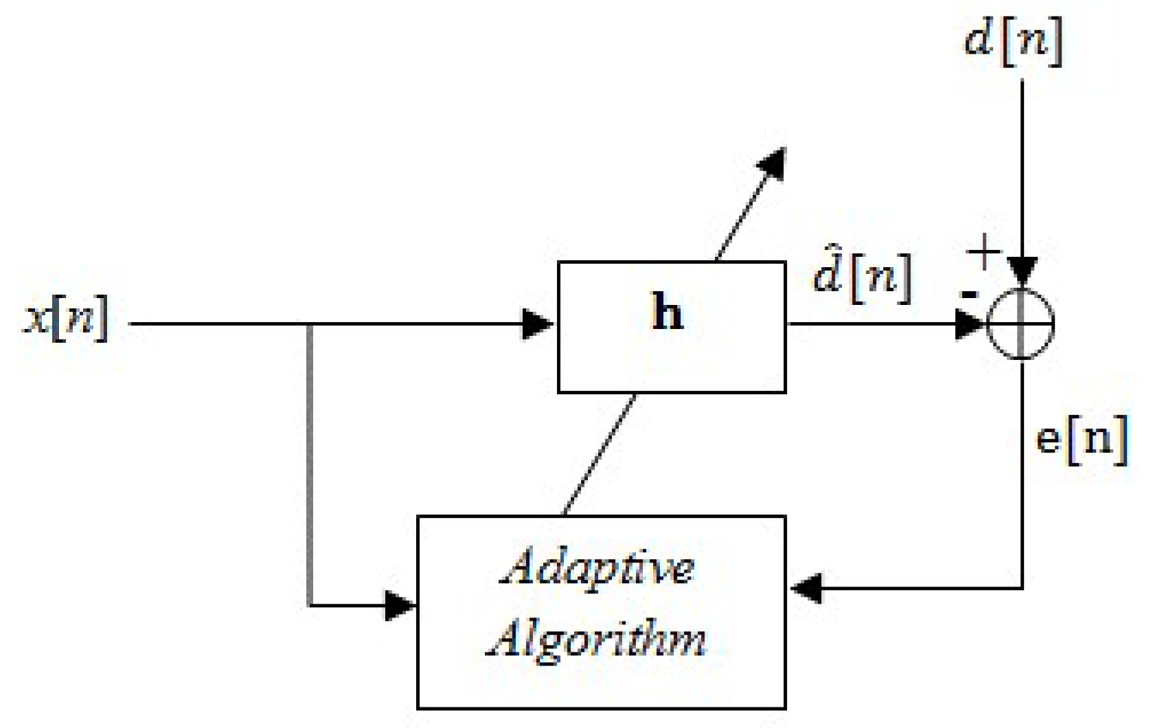
Example 2

(Adaptive Filtering). In a general setting, let us consider an adaptive filtering problem in Figure 2, where a measurement vector $\mathbf{x}\left[n\right]\triangleq {\left[x_1\left[n\right],x_2\left[n\right],\dots ,x_N\left[n\right]\right]}^T$ is used to construct an estimate, $\widehat{\mathbf{d}}\left[n\right]\triangleq (\mathbf{h}\star \mathbf{x})\left[n\right]$, of the desired signal $\mathbf{d}\left[n\right]$ by a linear shift-variant filter $\mathbf{h}\left[n\right]$ [7]. Then, the task is to synthesize an adaptive algorithm to update the filter $\mathbf{h}\left[n\right]$ such that the estimation error $\mathbf{e}\left[n\right]\triangleq \left(\mathbf{d}\left[n\right]-\widehat{\mathbf{d}}\left[n\right]\right)\to \mathbf{0}$ as $n\to \infty$. Using Lemma 1, this could be achieved if $\mathbf{e}\in {\ell }^p$ for some $p\in [1,\infty )$ in the adaptive algorithm.

If a dynamical system at any time n does not depend on the future (i.e., the system is only dependent on the past and the present) input(s), then the system is said to be causal [15] and the convolution in Equation (1) reduces to

$$\mathbf{y}\left[n\right]=\sum _{k=-\infty }^n\mathbf{h}[n-k]\mathbf{u}\left[k\right]$$

(2)

If, in addition, $\mathbf{u}\left[k\right]=\mathbf{0}\forall k<0$, then it follows that

$$\mathbf{y}\left[n\right]=\sum _{k=0}^n\mathbf{h}[n-k]\mathbf{u}\left[k\right]$$

(3)

2.2. Hardy Spaces and Spectral Factorization for Signal Processing

This subsection introduces the concept of Hardy spaces ${\mathcal{H}}^p$, $1\le p\le \infty$, which constitute a class of Banach spaces with a special structure; this structure is very useful for digital signal processing [3]. In particular, ${\mathcal{H}}^2$ and ${\mathcal{H}}^{\infty }$ spaces are of importance in robust control theory and it will be seen later in this section that the ${\mathcal{H}}^1$ space also plays an important role for power spectrum factorization in digital signal processing.

Recalling that, for a linear shift-invariant system with an impulse response $\mathbf{h}\left[n\right]$ and input $\mathbf{u}\left[n\right]$, the output $\mathbf{y}\left[n\right]$ is obtained by convolution [14] as: $\mathbf{y}=\mathbf{h}\ast \mathbf{u}$. Then, by setting $z\triangleq e^{i\omega }$ where $\omega$ is the frequency in radians, the z-transform of the impulse response $\mathbf{h}$ is defined as:

$$H\left(z\right)=\sum _{n=-\infty }^{\infty }h\left[n\right]z^{-n}$$

(4)

which is known as the system transfer function (The one-dimensional z-transform of the discrete-time impulse response $h\left[k\right]$ is the ratio of two polynomials: $H\left(z\right)\triangleq \frac{N\left(z\right)}{D\left(z\right)}$, where the degree of $N\left(z\right)$ is less than or equal to that of $D\left(z\right)$ for physically realizable systems. However, for the multi (i.e., n)-dimensional z-transform, where $n\in \mathbb{N}/\{1\}$, the resulting transfer function is given as the ratio of the numerator and denominator multinomials:

$$H\left(z\right)\triangleq \frac{N(z_1,\cdots ,z_n)}{D(z_1,\cdots ,z_n)}$$

The analysis of multi-dimensional z-transform (e.g., in signal processing of spatio-temporal processes) is significantly more complicated than that of one-dimensional z-transform, because the fundamental theorem of algebra may not be applicable to multinomials while it is always applicable to polynomials.) in the z-domain.

The system $H\left(z\right)$ is stable if the sum in Equation (4) converges, and the region of convergence (ROC) is called the stablity region, where all poles of $H\left(z\right)$ are located inside the unit circle with its center at zero in the complex z-plane. The system is said to be minimum-phase if all zeros of $H\left(z\right)$ are located inside the unit circle. If all zeros of $H\left(z\right)$ are located outside the unit circle, then the system is called maximum-phase [16], and the system is called non-minimum-phase if at least one zero of $H\left(z\right)$ is located outside the unit circle.

Definition 3

(Analytic Functions). Let $D_r\left(z_0\right)\triangleq \{z\in \mathbb{C}:|z-z_0|<r\}$ be the open disc of radius $r>0$ with center at $z_0\in \mathbb{C}$. A complex-valued function $f\left(r{e}^{i\theta }\right)$, where $\theta \in [0,2\pi )$, is said to be analytic in $D_r\left(z_0\right)$ if the derivative of $f\left(r{e}^{i\theta }\right)$ exists at each point of $D_r\left(z_0\right)$.

Given $p\in [1,\infty ]$, the Hardy space ${\mathcal{H}}^p$ is a set of analytic functions $f\left(r{e}^{i\theta }\right)$ with bounded ${\mathcal{H}}^p$-norm defined as:

$${\parallel f\parallel }_{H^p}\triangleq \underset{r\in (0,1)}{sup}\frac{1}{2\pi }{\int }_0^{2\pi }d\theta {\left|f\left(r{e}^{i\theta }\right)\right|}^{\frac{1}{p}}\mathrm{for}p\in [1,\infty )$$

$${\parallel f\parallel }_{H^{\infty }}\triangleq \underset{\left|z\right|<1}{sup}\left|f\left(z\right)\right|,\mathrm{for}p=\infty$$

The following theorem, due to Paley and Wiener [14], presents a fundamental result in the ${\mathcal{H}}^1$-space, which is important for spectral factorization in signal processing and for innovation representation of random processes.

Theorem 4

(Paley-Wiener). Let $S\left(z\right)$ be a complex-valued function of the complex variable z. If $ln\left(S\right)\in H^1$, then there exists a real positive constant $K_0$ and a complex-valued function $H_{ca}\left(z\right)$ corresponding to a causal stable system with a causal stable inverse such that

$$S\left(z\right)=K_0{H}_{ca}\left(z\right)H_{ca}^{her}(1/\overline{z})$$

(5)

where the superscript “her" indicates the Hermitian, i.e., complex conjugate of transpose of a vector/matrix, and $\overline{z}$ is the complex conjugate of z. If, in addition, $S\left(z\right)$ is a rational polynomial, the above factors $H_{ca}\left(z\right)$ and $H_{ca}^{her}(1/\overline{z})$ are minimum-phase and maximum-phase components, respectively. This is called the Paley-Wiener condition.

Proof. 

The proof of the Paley-Wiener Theorem is given in details by Therrian [14]. □

It follows from Equation (1) that, for a linear shift-invariant stable system with a deterministic LSI impulse response $\mathbf{h}\left[n\right]$ and a wide sense stationary (WSS) input signal $\mathbf{u}\left[n\right]$, the expected value of the output $\mathbf{y}\left[n\right]$ is:

$$E\left[\mathbf{y}\left[n\right]\right]=\sum _{k=-\infty }^{\infty }\mathbf{h}[n-k]E\left[\mathbf{u}\left[k\right]\right]$$

(6)

Since the input $\mathbf{u}$ is WSS, expected values, $m_y$ and $m_u$, of the output $\mathbf{y}$ and input $\mathbf{u}$, respectively, are related as:

$$m_y=\left(\sum _{k=-\infty }^{\infty }\mathbf{h}\left[k\right]\right)m_u$$

(7)

Autocorrelation of a random vector $\mathbf{x}\left[k\right]$ is denoted as ${\mathbf{r}}_{xx}\left[k\right]\triangleq E\left[\mathbf{x}\left[k\right]{\mathbf{x}}^{her}\left[k\right]\right]$, and the cross-correlation between the output $\mathbf{y}$ and the input $\mathbf{u}$ is given by

$${\mathbf{r}}_{yu}[n_1,n_0]=\sum _{k=-\infty }^{\infty }\mathbf{h}[n_1-k]{\mathbf{r}}_{uu}[k-n_0]$$

(8)

The above equation leads to the following important relations between correlation functions [14]:

$$r_{yu}[\ell ]=\mathbf{h}[\ell ]\ast r_{uu}[\ell ]\mathrm{and}{\mathbf{r}}_{yy}[\ell ]=\mathbf{h}[\ell ]\ast {\mathbf{r}}_{uu}[\ell ]\ast {\mathbf{h}}^{her}[-\ell ]$$

(9)

where the superscript her indicates the Hermitian, i.e., the complex conjugate of transpose of a vector/matrix.

The Fourier transform of ${\mathbf{r}}_{xx}\left[k\right]$ for a WSS random sequence $\mathbf{x}\left[k\right]$ is called the power spectral density function [7], defined as:

$$S_{xx}\left(e^{i\omega }\right)\triangleq \sum _{k=-\infty }^{\infty }{e}^{-i\omega k}{\mathbf{r}}_{xx}\left[k\right]$$

(10)

and its inverse Fourier transform, which is equal to the autocorrelation function, is obtained as:

$$r_{xx}\left[k\right]={\displaystyle \frac{1}{2\pi }}{\int }_{-\pi }^{\pi }d\omega e^{i\omega k}{S}_{xx}\left(e^{i\omega }\right)$$

(11)

The z-transform of the autocorrelation function for a WSS random sequence $\mathbf{x}\left[n\right]$ is called the complex spectral density function and is defined as:

$$S_{xx}\left(z\right)\triangleq \sum _{k=-\infty }^{\infty }{\mathbf{r}}_{xx}\left[k\right]z^{-k}$$

(12)

and its inverse is given by the contour integral

$${\mathbf{r}}_{xx}\left[k\right]={\displaystyle \frac{1}{2\pi i}}{\oint }_{C}dz{z}^{k-1}{S}_{xx}\left(z\right)$$

(13)

Since the autocorrelation function of a zero-mean white noise with variance ${\sigma }_w^2$ is given by ${\mathbf{r}}_w\triangleq {\sigma }_w^2\delta \left[k\right]$, the power spectral density is a constant ${\sigma }_w^2$ for a stationary white noise.

Using the property that the convolution in the time domain is a product in the Fourier transform domain and using Equation (9), it follows that

$$S_{yx}\left(e^{i\omega }\right)=H\left(e^{i\omega }\right)S_{xx}\left(e^{i\omega }\right)$$

(14)

where $H\left(e^{i\omega }\right)$ is the system transfer function (i.e., the Fourier transform of $\mathbf{h}\left[k\right]$). A few algebraic computations yield the following relation [14]:

$$S_{yy}\left(e^{i\omega }\right)=H\left(e^{i\omega }\right)S_{xx}\left(e^{i\omega }\right)H^{her}\left(e^{i\omega }\right)$$

(15)

In a similar manner, the following relations are obtained for the complex spectral density

$$\begin{array}{c}\hfill S_{yx}\left(z\right)=H\left(z\right)S_{xx}\left(z\right)\\ \hfill \mathrm{and}{S}_{yy}\left(z\right)=H\left(z\right)S_{xx}\left(z\right)H^{her}(1/\overline{z})\end{array}$$

(16)

Let us consider a WSS random sequence $\{x[k]\}$ whose complex spectral density satisfies the Paley-Wiener condition:

$$\ell n\left(S_{xx}\right)\in H^1,i.e.,{\int }_{-\pi }^{\pi }|\ell n{S}_{xx}\left(e^{i\omega }\right)|d\omega <\infty$$

(17)

Then, by Theorem 4, there exists a real positive constant $K_0$ and a complex-valued transfer function $H_{ca}\left(z\right)$ of a causal stable system with a causal stable inverse such that

$${\mathbf{r}}_{xx}\left(z\right)=K_0{H}_{ca}\left(z\right)H_{ca}^{her}(1/\overline{z})$$

(18)

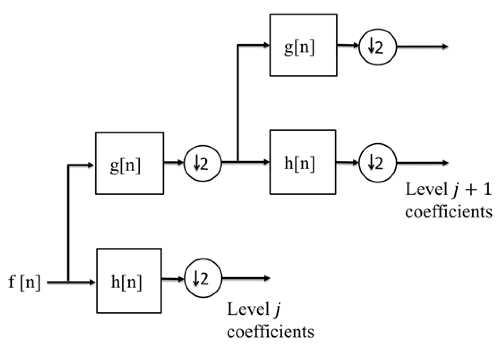
Remark 1.

A process, whose (complex) spectral density satisfies Equation (17), is called a regular process (see [7,14]). The spectral density factorization given by Equation (18) has important applications in signal processing. This includes what is called innovations representation of the random process [14], in view of which, any regular process can be realized as the output of a causal linear filter $H_{ca}\left(z\right)$ driven by a white noise with variance $K_0$ as shown in Figure 3.

It is worth-mentioning that this type of process covers a wide range of random processes. In particular, any process whose complex spectral density is a rational function of z is a regular process.

Example 3

([14]). Consider a random sequence $x\left[n\right]$ with a complex spectral density function:

$$S_{xx}\left(z\right)={\displaystyle \frac{-(1/a)}{z-(a+1/a)+z^{-1}}}$$

which could be re-written as:

$$S_{xx}\left(z\right)={\displaystyle \frac{1}{-az+(1+a^2)-a{z}^{-1}}}$$

$$={\displaystyle \frac{1}{(1-a{z}^{-1})}}.{\displaystyle \frac{1}{(1-az)}}$$

Using Paley-Wiener Theorem, $\mathbf{x}\left[n\right]$ can be realized as the output of a causally stable system, given by:

$$H_{ca}\left(z\right)={\displaystyle \frac{1}{1-a{z}^{-1}}}$$

(19)

excited by a zero-mean white noise with unit variance ${\sigma }^2=1$. It is important to note that since $S_x\left(z\right)$ is a rational polynomial, $H_{ca}\left(z\right)$ should be minimum-phase. This is the case for the one given by Equation (19).

Since the function can be factored as:

$$S_{xx}\left(z\right)={\displaystyle \frac{1}{-az+(1+a^2)-a{z}^{-1}}}={\displaystyle \frac{1}{(z-a)}}.{\displaystyle \frac{1}{(z^{-1}-a)}}$$

a possible pitfall here is to choose

$$H_{ca}\left(z\right)={\displaystyle \frac{1}{z-a}}={\displaystyle \frac{z^{-1}}{1-a{z}^{-1}}}$$

(20)

The term in Equation (20) is not minimum-phase because it has a zero at $\left|z\right|=\infty$. Moreover, the inverse ${\mathcal{H}}_{ca}^{-1}\left(z\right)=z-a$ is not causal. Therefore, the spectral factorization with $H_{ca}\left(z\right)$ given by Equation (20) is not physically realizable for the given random sequence $\{x[k]\}$.

As mentioned before, any random process whose complex spectral density is a rational polynomial is a regular process, and therefore it satisfies the Paley-Wiener condition. However, this is not a necessary condition for being a regular process as seen in the following example.

Example 4

([14]). Let a random sequence $x\left[n\right]$ have a complex spectral density $S_x\left(z\right)=e^{z+z^{-1}}$.

Then, the corresponding power spectral density $S_x\left(e^{i\omega }\right)=e^{2cos\omega }$ satisfies the Paley-Wiener condition that is given as:

$${\int }_{-\pi }^{\pi }d\omega |\ell n{S}_x\left(e^{i\omega }\right)|={\int }_{-\pi }^{\pi }d\omega \left|2cos\omega \right|<\infty$$

Therefore, the given random sequence is regular and has an innovations representation. The spectral factorization can be done as follows:

$$S_x\left(z\right)=1.e^{z^{-1}}.e^z$$

Then, the causal factor is given by

$$H_{ca}\left(z\right)=e^{z^{-1}}$$

(21)

which converges everywhere except at $z=0$. The impulse response of the filter is: $h_{ca}\left[n\right]=\frac{1}{n!}U\left[n\right]$, where $U\left[n\right]$ is the unit (discrete) step function, because

$$H_{ca}\left(z\right)=e^{z^{-1}}=\sum _{k=0}^{\infty }\frac{1}{k!}{z}^{-k}$$

So, the given random sequence can be realized as the output of a system, with a transfer function given by Equation (21), which is driven by a zero-mean white noise with a unit variance (i.e., ${\sigma }^2=1$).

In fact, a regular process is related to the corresponding predictable process that can be predicted with zero error. The relation between these two processes are given by the following fundamental theorem [7].

Theorem 5

(Wold Decomposition Theorem). A general random sequence $\mathbf{x}\left[n\right]$ can be written as the sum of two processes as:

$$\mathbf{x}\left[n\right]={\mathbf{x}}_r\left[n\right]+{\mathbf{x}}_p\left[n\right]$$

(22)

where ${\mathbf{x}}_r\left[n\right]$ is a regular process and ${\mathbf{x}}_p\left[n\right]$ is a predictable process, with ${\mathbf{x}}_r\left[n\right]$ being orthogonal to ${\mathbf{x}}_p\left[n\right]$, i.e., $E\{{\mathbf{x}}_r\left[m\right]{\mathbf{x}}_p^{her}\left[n\right]\}=0\forall m,n$.

Proof. 

The proof is given in [7]. □

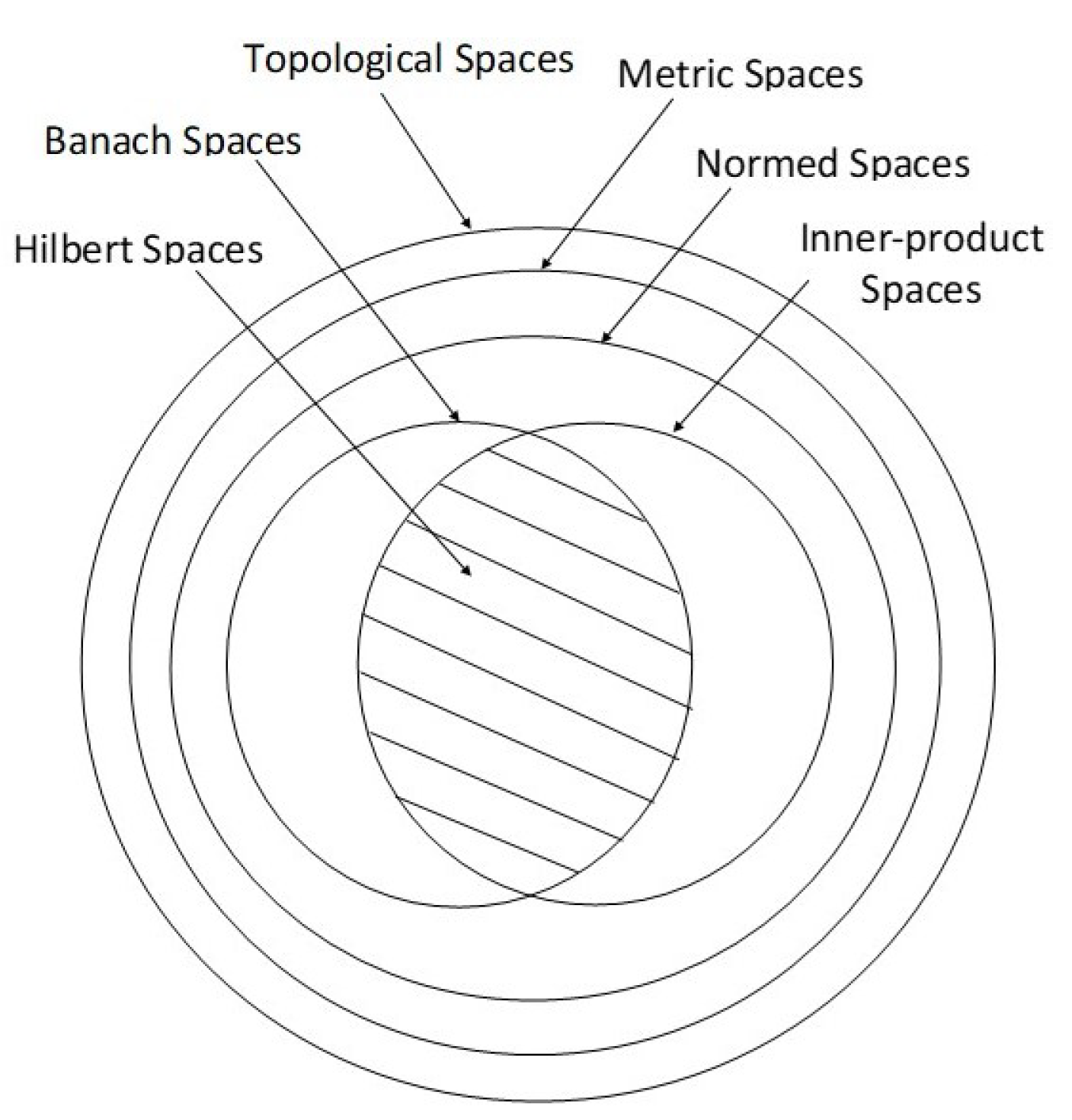
2.3. Weak Topology in a Banach Space

It follows from the Appendix A that an appropriate collection of open sets in a metric space defines its topology, and such a topology is called a metric topology or strong topology. In fact, a base for the strong topology on a Banach space X is the collection of all open balls, i.e., sets of the form:

$$\{f\in X:\parallel f-g\parallel <r\},$$

(23)

where the center g is a vector/function in X and the radius r is a positive real number. In this topology, convergence of a sequence, $\{f_n\}$, of functions in X to a limit g in X is referred to as strong convergence, which implies that $\parallel g-f_n\parallel \to 0$ and is denoted by $f_n\stackrel{s}{\to }g$. Besides strong convergence, other notions of convergence (e.g., weak convergence and uniform convergence) have been introduced in the literature, which play significant roles in the theory of Banach algebra [1].

We now introduce the notions of weak convergence and weak topology. Given a Banach space X over a field $\mathbb{K}$, let $\mathcal{F}\triangleq \{F_1,F_2,\cdots \}$ be a set of bounded linear functionals (A functional is a mapping of a vector space X into its field $\mathbb{K}$. Then, the set of all linear bounded (equivalently, linear continuous) functionals in X is called the dual space $X^{\ast }$.) on X, i.e., each $F_i$ is an element in the dual space $X^{\star }$ and hence $\mathcal{F}\subset X^{\star }$. Given an $\epsilon >0$ and a vector/function $f_0\in X$, let us define the set:

$$\mathsf{\Omega }(\mathcal{F};f_0,\epsilon )\triangleq \{f\in X;|F_i\left(f\right)-F_i\left(f_0\right)|<\epsilon ,\forall F_i\in \mathcal{F}\}$$

(24)

A class of such sets is obtained by varying $\epsilon \to 0^{+}$ in Equation (24) to establish the notions of weak convergence and weak topology. Some of these convergence concepts in the space of linear bounded operators are briefly explained in the following definitions, which are introduced for different notions of convergence of sequences $\{T^k\}$ of bounded linear operators in Banach spaces.

Definition 4

(Convergence in operator norm or uniform convergence). Let $T^k\in BL(V,V)$ be a bounded linear operator from V into V. Then, the sequence $\{T^k\}$ converges to some $T\in BL(V,V)$ in the operator norm (also called uniform convergence) if the induced norm $\parallel (T-T^k){\parallel }_{ind}\triangleq {lim}_{k\to \infty }{sup}_{{\parallel x\parallel }_V=1}{\parallel (T-T^k)x\parallel }_V=0$, which is denoted as: $T^k\stackrel{u}{\to }T$.

Definition 5

(Strong convergence). Let $T^k\in BL(V,V)$ be a bounded linear operator from V into V. Then, the sequence $\{T^k\}$ converges strongly to some $T\in BL(V,V)$ if ${lim}_{k\to \infty }{\parallel (T-T^k)x\parallel }_V=0\forall x\in V$, which is denoted as $T^k\stackrel{s}{\to }T$.

Definition 6

(Weak convergence). Let $T^k\in BL(V,V)$ be a bounded linear operator from V into V. Then, the sequence $\{T^k\}$ converges weakly to some $T\in BL(V,V)$ if

$$\forall F\in V^{\star }\forall x\in V,\underset{k\to \infty }{lim}\left|\left(F\left(Tx\right)-F\left(T^{k}x\right)\right)\right|=0,$$

which is denoted as $T^k\stackrel{w}{\to }T$.

Remark 2

(Convergence in operator norm). ⇒ (Strong convergence) ⇒ (Weak Convergence). The converse is not true, in general.

To show ($T^k\stackrel{u}{\to }T$) ⇒ ($T^k\stackrel{s}{\to }T$), we proceed as:

$\forall x\in V$, $\parallel (T-T^k){x\parallel }_V\le \parallel (T-T^k){\parallel }_{ind}{\parallel x\parallel }_V$ implies that, given $T^k\stackrel{u}{\to }T$, i.e., ${lim}_{k\to \infty }{\parallel (T-T^k)\parallel }_{ind}=0$, it follows that ${lim}_{k\to \infty }{\parallel (T-T^k)x\parallel }_V=0\forall x\in V,i.e.,T^k\stackrel{s}{\to }T$.

To show ($T^k\stackrel{s}{\to }T$) ⇒ ($T^k\stackrel{w}{\to }T$):, we proceed as:

$T^k\stackrel{s}{\to }T\Rightarrow {lim}_{k\to \infty }{\parallel (T-T^k)x\parallel }_V=0\forall x\in V$. Let $f\in V^{\star }$; then, it follows from linearity and boundedness of the functional f that $\left|f\left(x\right)\right|\le {\parallel f\parallel }_{ind}{\parallel x\parallel }_V$. Therefore, $\forall x\in V\forall f\in V^{\star },{lim}_{k\to \infty }\left|\left(f\left(Tx\right)-f\left(T^{k}x\right)\right)\right|=0\Rightarrow T^k\stackrel{w}{\to }T$

We demonstrate the falsity of the converse by two counterexamples, one for each case.

(Strong convergence) ⇏ (Convergence in operator norm): Let us define $x\triangleq \{{\xi }_n:n\in \mathbb{N}\}$ and a sequence of bounded linear operators $T^k:{\ell }_2\to {\ell }_2\forall k\in \mathbb{N}$ as:

$$T^{k}x\triangleq \{\underset{firstkterms}{\underbrace{0,0,0,\cdots ,0}},{\xi }_{k+1},{\xi }_{k+2},\cdots \}$$

Therefore, $T^k$ is a bounded linear operator, i.e., $T^k\in BL({\ell }_2,{\ell }_2)$. Since $x\in {\ell }_2$, it follows that

$$\underset{k\to \infty }{lim}\parallel T^k{x\parallel }_{{\ell }_2}=0\Rightarrow \underset{k\to \infty }{lim}\parallel T^k\parallel {=}_s{\mathbf{0}}_{BL({\ell }_2,{\ell }_2)}$$

However, the limit may not converge in the induced norm, ${lim}_{k\to \infty }{sup}_{{\parallel x\parallel }_{{\ell }_2}=1}{\parallel T^{k}x\parallel }_{{\ell }_2}=1$ as seen by choosing $x=\{\underset{firstkterms}{\underbrace{0,0,0,\cdots ,0}},{\xi }_{k+1},{\xi }_{k+2},\cdots \}$ with ${\parallel x\parallel }_{{\ell }_2}=1\Rightarrow {lim}_{k\to \infty }\parallel T^k\parallel {\ne }_u{\mathbf{0}}_{BL({\ell }_2,{\ell }_2)}$.

Therefore, (Strong convergence) ⇏ (Convergence in operator norm).

(Weak convergence) ⇏ (Strong convergence): Let us define a sequence of bounded linear operators $T^k:{\ell }_2\to {\ell }_2\forall k\in \mathbb{N}$ as:

$$T^{k}x=\{\underset{firstkterms}{\underbrace{0,0,0,\cdots ,0}},{\xi }_1,{\xi }_2,\cdots \}$$

where $x\triangleq \{{\xi }_n:n\in \mathbb{N}\}$. It is given that $\{T^k\}$ is a sequence of bounded linear operators, i.e., each $T^k\in BL({\ell }_2,{\ell }_2)$. Furthermore, in this Hilbert space setting, it follows from the Riesz Representation Theorem that every $f\in {\ell }_2^{\star }$ can be represented as:

$$f\left(x\right)={\langle x,y\rangle }_{{\ell }_2}=\sum _{n=1}^{\infty }{\xi }_n{\eta }_n,\mathit{where}y=\{{\eta }_k:k\in \mathbb{N}\}$$

It follows by Cauchy-Schwarz inequality that, as $k\to \infty$

$$|f\left(T^{k}x\right){|}^2=|\langle T^{k}x,y\rangle {|}^2\le \sum _{n=1}^{\infty }|{\xi }_n{|}^2\sum _{m=k+1}^{\infty }{|{\eta }_m|}^2\to 0$$

However,

$$\parallel T^k{x\parallel }_{{\ell }_2}={\parallel x\parallel }_{{\ell }_2}\forall k\in \mathbb{N}\Rightarrow \exists x\ne {\mathbf{0}}_{{\ell }_2}\mathit{such}\mathit{that}$$

$$\underset{k\to \infty }{lim}{\parallel T^{k}x\parallel }_{{\ell }_2}\ne 0\Rightarrow \underset{k\to \infty }{lim}{T}^k{\ne }_s{\mathbf{0}}_{BL({\ell }_2,{\ell }_2)}$$

Therefore, (Weak convergence) ⇏ (Strong convergence).

Remark 3.

It is noted that, for finite-dimensional vector spaces, the notions of strong convergence and weak convergence are indistinguishable. Equivalently, we make the following statement:

In a finite-dimensional Banach space V, the weak topology generated by $V^{\star }$ is the same as the strong topology generated by V.

However, in the analysis of stochastic processes, we deal with infinite-dimensional spaces of signal functions, which may not have the same criteria for weak convergence and strong convergence. This is especially applicable to statistical signal processing, where the expectation of the estimation error is required to weakly converge to zero without having the strong convergence of the error signal itself to zero.

Based on the concept of weak convergence, weak topology is defined as follows:

Definition 7

(Convergence in weak topology). Given a Banach space X, let there be a class of bounded linear functionals $\mathcal{F}\subseteq X^{\star }$, and let $\Im \left(\mathcal{F}\right)$ be the topology in X generated by $\mathcal{F}$. Then, for a given vector/function $g\in X$, a sequence $\{f_n\}\subset X$ is said to converge to g in the weak topology $\Im \left(\mathcal{F}\right)$, denoted as $f_n\stackrel{w}{\to }g$ in $\Im \left(\mathcal{F}\right)$, provided that $F_{\alpha }\left(f_n\right)$ converges strongly to $F_{\alpha }\left(g\right)$, denoted as $F_{\alpha }\left(f_n\right)\stackrel{s}{\to }{F}_{\alpha }\left(g\right)\forall F_{\alpha }\in \mathcal{F}$.

Weak convergence in Definition 7 is a generalization of weak convergence as introduced in the functional analysis literature, which implies that a sequence $\{f_n\}\subset X$ converges weakly to some $g\in X$ if $G\left(f_n\right)\stackrel{s}{\to }G\left(g\right)\forall G\in X^{\star }$ [10].

Remark 4.

The concept of topological spaces and weak topology are important for learning using statistical invariants (LUSI). In a machine learning paradigm, learning machines often compute statistical invariants for specific problems with the objective of reducing the expected values of errors in a such way that preserves these invariants. In contrast to classical machine learning that employs the mechanism of strong convergence for approximations to the desired function, LUSI can significantly increase the rate of convergence by combining the mechanisms of strong convergence and weak convergence [17]. Furthermore, the notion of weak topology is also important when dealing with shift spaces for signal analysis that uses symbolic dynamics, as explained in [18,19].

3. Hilbert Spaces for Signal Processing

This section introduces the concept of Hilbert spaces, which forms the backbone in the disciplines of signal processing and other fields of engineering. Details are provided in many textbooks such as Naylor and Sell [2].

Definition 8

(Hilbert Spaces). Let a vector space X be defined over a field $\mathbb{K}$, which is either $\mathbb{R}$ or $\mathbb{C}$. A function $\langle •,•\rangle :X\times X\to \mathbb{K}$ is called an inner product if, for $\forall x,y,z\in X$ and $\forall \alpha \in \mathbb{K}$, the following conditions hold:

1. 

(positive definiteness) $\langle x,x\rangle >0$ when $x\ne \mathbf{0}$;

2. 

(additivity) $\langle (x+y),z\rangle =\langle x,z\rangle +\langle y,z\rangle$;

3. 

(homogeneity) $\langle \alpha x,y\rangle =\alpha \langle x,y\rangle$;

4. 

(symmetry) $\langle x,y\rangle =\overline{\langle y,x\rangle }$

Then, $\left(X,\langle •,•\rangle \right)$ is called a inner product space or a pre-Hilbert space, and a complete inner product space (i.e., where every Cauchy sequence converges in the space) is called a real (resp. complex) Hilbert space, depending on whether the vector space is defined over $\mathbb{R}$ (resp. $\mathbb{C}$).

The following two properties are immediate consequences of the four properties in Definition 8:

• $\langle x,(y+z)\rangle =\langle x,y\rangle +\langle x,z\rangle$;
• $\langle x,\alpha y\rangle =\overline{\alpha }\langle x,y\rangle$;

It is also noted that every inner product space is a normed space with the norm $\parallel x\parallel \triangleq \sqrt{\langle x,x\rangle }\forall x\in X$ [2].

Example 5.

An example of a Hilbert space is the ${\ell }^2$ space of square-summable sequences. Given two sequences $x=\{x_n\}$ and $y=\{y_n\}$ in ${\ell }^2$, the inner product is given by $\langle x,y\rangle \triangleq {\sum }_{n=-\infty }^{\infty }{\overline{x}}_n{y}_n$. Two vectors x and y in a Hilbert space H are said to be orthogonal if $\langle x,y\rangle =0$. Given a subspace $V\subset H$, its orthogonal complement is denoted as: $V^{\perp }\triangleq \{u\in H:\langle u,v\rangle =0\forall v\in V\}$; consequently, $V\oplus V^{\perp }=H$

Hilbert spaces have many common interesting properties that make them to be important in optimization theory [12]. As we will see in the sequel, these properties form the core of many fundamental results in adaptive and statistical signal processing, and they are established through the following theorem.

Theorem 6

(Riesz Representation Theorem [2,5]). Let H be a a Hilbert space. Then, for every bounded linear functional $f:H\to \mathbb{C}$, there exists a unique $y\in H$ such that $f\left(x\right)={\langle y,x\rangle }_H$ $\forall x\in H$.

Proof. 

The proof is given in [2] in pp. 345–346. □

Remark 5.

For the Hilbert spaces ${\ell }^2$ (resp. $L^2$), this result can be obtained by using a theorem [5], which states that, given $p\in [1,\infty )$, ${\ell }^q$ (resp. $L^q$) is isometrically isomorphic to the dual space of ${\ell }^p$ (resp. $L^p$) provided that ${\displaystyle \frac{1}{p}}+{\displaystyle \frac{1}{q}}=1$, where q is called the conjugate of p. Since the conjugate of $p=2$ is $q=2$, it follows that ${\ell }^2$ is isometrically isomorphic to ${\left({\ell }^2\right)}^{\ast }$, and similar relations hold for $L^2$ and ${\left(L^2\right)}^{\ast }$ (for example, see [3]); hence, ${\ell }^2$ and $L^2$ are reflexive. Generalization of this fact is stated as the following theorem.

Theorem 7.

Every Hilbert space is reflexive, i.e., H is isometrically isomorphic to its dual space $H^{\ast }$.

The proof of this theorem is given in many textbooks on functional analysis (e.g., [5,10,20]).

Another important property of Hilbert spaces, which is widely used in signal processing in combination with the previous two properties (see Theorens 6 and 7), is given as the following theorem [5]:

Theorem 8

(Orthogonal Projections). Let H be a Hilbert space, and let $V\subset H$ be a closed subspace of H, implying that V is also a Hilbert space. Then, it follows that

(i) $H=V\oplus V^{\perp }$. That is, given $x\in H$, there exists a unique pair $v\in V$ and $u\in V^{\perp }$ such that $x=u+v$.

(ii) $v_V\left(x\right)$ is the unique vector in V having minimal distance from a vector $x\in H$, while $u_{V^{\perp }}\left(x\right)$ is the unique vector in $V^{\perp }$ having minimal distance from x.

(iii) The orthogonal projections $x\mapsto v_V\left(x\right)$ and $x\mapsto u_{V^{\perp }}$ are linear continuous operators, with norm $\le 1$.

Proof. 

The proof is given in [2] in pp. 300–305. □

Remark 6.

It follows from Theorem 8 that the decomposition in Equation (22) in Section 2 is indeed unique. Based on this fact, any random process generally consists of two unique orthogonal components; a predictable component and an unpredictable component. That is, if one wants to predict $x\left[n\right]$ by using N past observations $\{x_{n-N},x_{n-N+1},\dots ,x_{n-1}\}$, then let $\widehat{x}\left[n\right]={\sum }_{k=1}^N{a}_{k}x[n-k]$ denote an optimal linear prediction of $x\left[n\right]$. Such a prediction can be obtained by applying the orthogonality principle, where the prediction error is given by $e\left[n\right]\triangleq x\left[n\right]-\widehat{x}\left[n\right]=x\left[n\right]-{\sum }_{k=1}^N{a}_{k}x[n-k]$, and the process $x\left[n\right]$ can be expressed as:

$$x\left[n\right]=\widehat{x}\left[n\right]+e\left[n\right]=\widehat{x}\left[n\right]+\left(x\left[n\right]-\sum _{k=1}^N{a}_{k}x[n-k]\right)$$

Hence, the part $\widehat{x}\left[n\right]$ represents the predictable part of $x\left[n\right]$, which corresponds to $x_p\left[n\right]$ in Wold decomposition Theorem in Equation (22), while the error $e\left[n\right]$ represents the unpredictable part of $x\left[n\right]$, which corresponds to $x_r\left[n\right]$ in Wold decomposition Theorem. That is, the regular process represents the difference between the random process and its optimal prediction. Therefore, the output of $H_{ca}^{-1}\left(z\right)$ represents only the new part of information, brought by $x\left[n\right]$, which cannot be extracted from the past observations. Therefore, the output of $H_{ca}^{-1}\left(z\right)$ is called innovations process as depicted in Figure 3b.

Another interesting result on Hilbert spaces is stated in the following theorem [2,10].

Theorem 9

(Bessel Inequality). Let H be a Hilbert space and let $V=span\{e_1,e_2,\dots \}$ be a subspace of H. If $P_V:H\to V$ denotes the orthogonal projection of elements in H into V, then, the Bessel inequality

$$\sum _{k\ge 1}|(x,e_k){|}^2=\parallel P_V{x\parallel }^2\le {\parallel x\parallel }^2$$

(25)

holds for every $x\in H$. Moreover,

$$\sum _{k\ge 1}(x,e_k)e_k=P_{V}x$$

(26)

This theorem has an important implication to signal processing as explained in the following subsection.

3.1. Fourier Series Expansion in a Hilbert Space

In the Hilbert space $L^2\left([t_0,t_0+T]\right)$, which is the space of all square-integrable periodic functions $f:[t_0,t_0+T]\to \mathbb{C}$ with $t_0\in \mathbb{R}$ with a period $T\in (0,\infty )$, an inner product is defined as:

$$\langle f,g\rangle \triangleq {\int }_{t_0}^{t_0+T}dt\overline{f}\left(t\right)g\left(t\right)\forall f,g\in L^2\left([t_0,t_0+T]\right)$$

(27)

Let the set of functions $S\triangleq \{{\phi }_n\left(t\right)$, $n\in \mathbb{Z}\}$, where

$$\begin{array}{c}\hfill {\phi }_n\left(t\right)\triangleq {\displaystyle \frac{e^{i{\omega }_{n}t}}{\sqrt{T}}};{\omega }_n\triangleq 2\pi n/T\forall n\in \mathbb{Z}\end{array}$$

(28)

Then, it follows by setting $T=2\pi$ that

$$\langle {\phi }_m,{\phi }_n\rangle =\frac{1}{2\pi }{\int }_{-\pi }^{\pi }dt\overline{e^{imt}}{e}^{int}=\left\{\begin{array}{cc}1\hfill & \mathrm{if}m=n\hfill \\ 0,\hfill & \mathrm{if}m\ne n\hfill \end{array}\right.$$

$$\mathrm{and}\mathrm{thus}\langle {\phi }_m,{\phi }_n\rangle ={\delta }_{mn}\forall m,n\in \mathbb{Z}$$

(29)

where ${\delta }_{mn}$ is called the Kronecker delta. Moreover, it turns out that $span\left(S\right)$ is dense in $L^2\left([t_0,t_0+T]\right)$, i.e., the completion $\overline{span\left(S\right)}=L^2\left([t_0,t_0+T]\right)$ (see [10]). Therefore, given any $f\in L^2\left([t_0,t_0+T]\right)$, there exists a sequence of scalars $\{c_k\}\subset \mathbb{C}$ such that

$${lim}_{N\to \infty }{\parallel f-{\sum }_{k=-N}^N{c}_k{\phi }_k\parallel }_{L^2}=0$$

That is,

$$f\left(t\right)\stackrel{ms}{=}\sum _{k=-\infty }^{\infty }{c}_k{\phi }_k\left(t\right)$$

(30)

Therefore, $\{{\phi }_n\left(t\right);n\in \mathbb{Z}\}$ is in fact an orthonormal basis of $L^2\left([t_0,t_0+T]\right)$. The infinite sum ${\sum }_{k=-\infty }^{\infty }{c}_k{\phi }_k$ is called the Fourier series expansion of f, where $\{c_k\}$ are the Fourier coefficients. Using Equation (29) and taking the inner product of both sides of Equation (30) by ${\phi }_n$, for any $n\in \mathbb{Z}$, yields

$$c_n\stackrel{ms}{=}\langle {\phi }_n,f\left(t\right)\rangle$$

(31)

Hence, Equation (30) can be rewritten in the following form:

$$f\left(t\right)\stackrel{ms}{=}\sum _{n=-\infty }^{\infty }\langle {\phi }_n,f\left(t\right)\rangle {\phi }_n\left(t\right)$$

(32)

Moreover, it follows from Equation (26) in Theorem 9 that

$${\parallel f\parallel }_{L_2}^2=\sum _{k=-\infty }^{\infty }{\left|c_k\right|}^2$$

(33)

In view of Equation (32), Fourier expansion of any square integrable signal $f\in L^2\left([t_0,t_0+T]\right)$ can be decomposed as a linear combination of harmonic modes ${\phi }_k$ with frequencies ${\omega }_k$ [21], where each Fourier coefficient $c_k$ represents the signal’s component associated with each mode ${\phi }_k$. Furthermore, Equation (33) reveals how signal’s energy ${\parallel f\parallel }_{L_2}^2$ is distributed over the signal’s components $\{c_k\}$ and demonstrates an important fact that, for each component $c_k$, the value $|c_k{|}^2$ represents a part of the signal’s energy contributed by the component $c_k$. This fact plays a central role in signal compression, where a signal $f\in L^2\left([t_0,t_0+T]\right)$ is approximated by using as few Fourier coefficients as possible; this is accomplished with a minimum approximation error by considering those values of $\{c_k\}$ with large magnitudes and by discarding those coefficients with small magnitudes.

Now we summarize the main results of Fourier series expansion of periodic functions as a theorem.

Theorem 10

(Fourier Series Theorem). Let $\{{\phi }_n\}$ be an orthonormal set in a Hilbert space H. Then, the following statements are equivalent:

1. 

$\{{\phi }_n\}$ is an orthonormal basis of H, i.e., $\{{\phi }_n\}$ is a complete orthonormal set in H.

2. 

(Fourier series expansion) Any vector $x\in H$ can be expanded as: $x\stackrel{ms}{=}{\sum }_{n\in \mathbb{N}}\langle x,{\phi }_n\rangle {\phi }_n$. Note: The inner products $\langle x,{\phi }_n\rangle$ are called Fourier coefficients of the vector x.

3. 

(Parseval Equality) For any two vectors $x,y\in H$, the inner product: $\langle x,y\rangle ={\sum }_{n\in \mathbb{N}}\langle x,{\phi }_n\rangle$ $\overline{\langle y,{\phi }_n\rangle }$

4. 

The norm: ${\parallel x\parallel }^2={\sum }_{n\in \mathbb{N}}{\left|\langle x,{\phi }_n\rangle \right|}^2\forall x\in H$

5. 

Let U be a subspace of H such that U contains the sequence $\{{\phi }_n\}$. Then, U is dense in H, i.e., $\overline{U}=H$.

Proof. 

The proof is given in [2] in pp. 307–312. □

3.2. Fourier Transform and Inverse Fourier Transform

For decomposition by Fourier series expansion, a function needs to be periodic as seen in Section 3.1. To extend this analysis to non-periodic functions, we first consider square-integrable periodic functions $f:[-T/2,T/2]\to \mathbb{C}$ and let $T\to \infty$ so that the restriction of periodic functions can be removed. Then, a combination of Equations (28) and (31) yields:

$$c_n\stackrel{ms}{=}{\displaystyle \frac{1}{\sqrt{T}}}{\int }_{-T/2}^{T/2}dt{e}^{-i{\omega }_{n}t}f\left(t\right)$$

(34)

and we define:

$${\widehat{f}}_T\left({\omega }_n\right)\triangleq \sqrt{T}{c}_n$$

(35)

Having $n\to \infty$ and ${\omega }_n\to \omega$ as $T\to \infty$, it follows that

$$\widehat{f}\left(\omega \right)\triangleq \underset{T,n\to \infty }{lim}{\widehat{f}}_T\left({\omega }_n\right)={\int }_{-\infty }^{\infty }dt{e}^{-i\omega t}f\left(t\right)$$

(36)

Now, we have Fourier transform of a signal $f\in L_2\left(\mathbb{R}\right)$. Since $L_2\left(\mathbb{R}\right)$ is the completion $\overline{L_1\left(\mathbb{R}\right)\cap L_2\left(\mathbb{R}\right)}$, we impose a mild restriction: $f\left(t\right)$ to be both absolute-value integrable and square-integrable. Nevertheless, this restriction is satisfied if f is an analytic function [21].

To obtain the inverse Fourier transform, we substitute Equations (28) and (35) into Equation (30), which yields

$$f\left(t\right)\stackrel{ms}{=}{\displaystyle \frac{1}{T}}\sum _{n=-\infty }^{\infty }{e}^{i{\omega }_{n}t}{\widehat{f}}_T\left({\omega }_n\right)$$

(37)

By defining ${\omega }_n\triangleq {\displaystyle \frac{n}{T}}$, we have $\Delta {\omega }_n\triangleq {\omega }_{n+1}-{\omega }_n={\displaystyle \frac{1}{T}}$. Then, substitution of ${\displaystyle \frac{1}{T}}$ into Equation (37) for $\Delta {\omega }_n$ yields

$$f\left(t\right)\stackrel{ms}{=}\sum _{n=-\infty }^{\infty }\Delta {\omega }_n{\widehat{f}}_T\left({\omega }_n\right)e^{i{\omega }_{n}t}$$

(38)

In the limits $T\to \infty$ and $n\to \infty$, Equation (38) becomes the inverse Fourier transform by using the Riemann sum [4]:

$$f\left(t\right)\stackrel{ms}{=}{\int }_{-\infty }^{\infty }d\omega e^{i\omega t}\widehat{f}\left(\omega \right)$$

(39)

Equation (33) can also be rewritten as:

$${\parallel f\parallel }_T^2=\sum _{n=-\infty }^{\infty }\Delta {\omega }_n{\left|{\widehat{f}}_T\left({\omega }_n\right)\right|}^2$$

(40)

This formula shows that a signal $f\left(t\right)\in L^2\left(\mathbb{R}\right)$ has, at any given time t, (possibly) uncountably many harmonic components distributed over the frequency range $-\infty <\omega <\infty$, and the magnitude of the harmonic component at a frequency $\omega$ is given by the signal’s Fourier transform $\widehat{f}\left(\omega \right)$. By taking the limits $T\to \infty$ and $n\to \infty$, it follows from Equations (33) and (34) that

$${\parallel f\parallel }_{L^2}^2={\int }_{-\infty }^{\infty }{dt\left|f\left(t\right)\right|}^2={\int }_{-\infty }^{\infty }d\omega |\widehat{f}{\left(\omega \right)|}^2={\parallel \widehat{f}\parallel }_{L^2}^2$$

(41)

The above relation is known as Plancherel’s theorem [3], which implies that the total energy of the signal, obtained in the time domain $t\in \mathbb{R}$ is re-distributed over the frequency domain $\omega \in \mathbb{R}$ such that the energy density at each frequency $\omega$ is $|\widehat{f}{\left(\omega \right)|}^2$. It is worth-mentioning that the inner products of two functions f and g in the time domain and the frequency domain is related by:

$${\langle f,g\rangle }_{L^2}={\langle \widehat{f},\widehat{g}\rangle }_{L^2}$$

(42)

which is known as Parseval’s identity [2].

In many signal processing applications, the signal f is complex-valued with a discrete domain, i.e., $f:\mathbb{Z}\to \mathbb{C}$. Then the discrete-time Fourier transform (DTFT) is given by:

$$\widehat{f}\left(\omega \right)=\sum _{n=-\infty }^{\infty }f\left(n\right)e^{-in\omega }$$

(43)

From Equation (43), it follows that

$$\begin{array}{c}\hfill |\widehat{f}\left(\omega \right)|=|\sum _{n=-\infty }^{\infty }f\left(n\right)e^{-in\omega }|\\ \hfill \le \sum _{n=-\infty }^{\infty }|f\left(n\right)e^{-in\omega }|=\sum _{n=-\infty }^{\infty }|f\left(n\right)|\end{array}$$

(44)

Therefore, a sufficient condition that guarantees the DTFT to be well-defined is that $f\in {\ell }^1$. The original sequence can be recovered from its DTFT by the inverse discrete-time Fourier transform (IDTFT)

$$f\left(n\right)={\displaystyle \frac{1}{2\pi }}{\int }_{-\pi }^{\pi }d\omega \widehat{f}\left(\omega \right)e^{in\omega }$$

(45)

Expressing the frequency from radians/sec to Hertz, i.e., by setting $\omega =2\pi \xi$, it follows that

$$f\left(n\right)={\int }_{-1}^{1}d\xi \widehat{f}\left(\xi \right)e^{i2\pi n\xi }$$

(46)

Although the Fourier transform plays a central role in signal analysis, it considers the time-averaged frequency behavior of the signal by integrating over the entire time domain $-\infty <t<\infty$. This property reduces the capability of capturing abrupt (i.e., rapid) changes which may occur in the signal; capturing such rapid changes in the signal is crucial in many applications, such as detection of faults and anomalies. In order to remedy this shortcoming of Fourier transform, the signal is integrated over a time window, instead of integrating over the entire time domain. This gives rise to the so-called windowed Fourier transform (WFT) which augments Fourier transform with a time-localization property that would provide information about the signal simultaneously in time and frequency domains [21,22]; a quantum-mechanics-based explanation of time-frequency localization is briefly explained in [23].

3.3. Windowed Fourier Transform in a Hilbert Space

A function $g:\mathbb{R}\to \mathbb{C}$ is said to have a compact support $B\subset \mathbb{R}$, and we say $supp\left(g\right)=B$ if g vanishes outside its compact domain B, i.e., $g\left(t\right)=0\forall t\notin B$. Given a function $f:\mathbb{R}\to \mathbb{C}$ and a $t\in \mathbb{R}$, let us define

$$f_t\left(u\right)\triangleq \overline{g}(u-t)f\left(u\right)$$

(47)

where $\overline{g}(·)$ is the complex conjugate of $g(·)$, and $supp\left(g\right)\subset [-T,0]$ for a positive real number T. Hence $f_t$ is a localized version of f and $supp\left(f_t\right)\subseteq [t-T,t]$ [21]. Then, the windowed Fourier transform (WFT) of f is the Fourier transform of $f_t$, which is given as:

$$\tilde{f}(\omega ,t)\triangleq {\widehat{f}}_t\left(\omega \right)={\int }_{-\infty }^{\infty }du{e}^{-i\omega u}{f}_t\left(u\right)$$

(48)

and the inverse WFT is obtained as:

$$f\left(t\right)={\displaystyle \frac{1}{{\parallel g\parallel }^2}}{\int }_{-\infty }^{\infty }d\omega {\int }_{-\infty }^{\infty }dt{g}_{\omega ,t}\left(u\right)\tilde{f}(\omega ,t)$$

(49)

where $g_{\omega ,t}\left(u\right)\triangleq e^{i\omega u}g(u-t)$.

By following Equation (48) and Equation (49), an inner product is defined as:

$$\langle g_{\omega ,t},f\rangle \triangleq \tilde{f}(\omega ,t)$$

(50)

Using Parseval’s identity in Equation (42), we have

$$\langle g_{\omega ,t},f\rangle =\langle {\widehat{g}}_{\omega ,t},\widehat{f}\rangle =\tilde{f}(\omega ,t)$$

(51)

Example 6.

An example of the window function g is:

$$g\left(u\right)=\left\{\begin{array}{cc}1+cos\left(\pi u\right),\hfill & -1\le u\le 1\hfill \\ 0,\hfill & \mathit{otherwise}\hfill \end{array}\right.$$

As mentioned in a previous subsection, if the signal is discrete, its DTFT is used to provide a frequency representation of the signal. Although the signal $f\left(n\right)$ in this case is discrete in the time domain, its DTFT is a continuous function of the frequency $\omega$. However, most of the devices used in signal processing are digital, and therefore it is more convenient to deal with a discrete frequency representation of the signal. Moreover, the discrete signal $f\left(n\right)$ in many cases represent a measurement data provided by some sensors, and such signals $f\left(n\right)$ are usually of finite length. The discrete Fourier transform (DFT) is a useful tool in signal processing that accommodates for these two issues as explained below.

Given a finite-length discrete signal $f:\{0,N-1\}\to \mathbb{C}$, the DFT is given as:

$$\tilde{f}\left[k\right]=\sum _{n=0}^{N-1}f\left[n\right]e^{-i2\pi kn/N}$$

(52)

The inverse discrete Fourier transform IDFT is:

$$f\left[n\right]={\displaystyle \frac{1}{N}}\sum _{k=0}^{N-1}\tilde{f}\left[k\right]e^{i2\pi kn/N}$$

(53)

Returning to the continuous WFT, if a function f is windowed over a time interval, the resulting WFT would have a time-localization property as seen earlier in the end of Section 3.2. Moreover, Equation (51)) shows that WFT of f localizes $\widehat{f}\left(\omega \right)$ to a neighborhhod of $\omega$. Therefore, WFT has both time and frequency localizations. However, due to the uncertainty principle, these two kinds of localization have different physical interpretations and are mutually exclusive in the sense that making a WFT $\tilde{f}(\omega ,t)$ sharper in time makes it more flat in frequency and vice versa [21,23]. Moreover, WFT is not efficient in scanning signals that involve time intervals much shorter or much longer than the window length T [21]. To address these issues, the notion of wavelet transform has been introduced in Section 3.4, which produce an efficient analysis tool to capture signal features occurring over short and long intervals.

3.4. Wavelet Transform in a Hilbert Space

The continuous wavelet transform (CWT) of a function $f:\mathbb{R}\to \mathbb{C}$ is defined as:

$$\tilde{f}(s,t)\triangleq {\int }_{-\infty }^{\infty }du{\overline{\psi }}_{s,t}\left(u\right)f\left(u\right)=\langle {\psi }_{s,t},f\rangle$$

(54)

where ${\psi }_{s,t}$, called the wavelet, is a scaled and translated version

$${\psi }_{s,t}\left(u\right)={\left|s\right|}^{-p}\psi \left({\displaystyle \frac{u-t}{s}}\right)\mathrm{where}s\ne 0$$

(55)

of what is called a mother (or basic) wavelet $\psi \triangleq {\psi }_{1,0}$; and ${\overline{\psi }}_{s,t}$ is the complex conjugate of ${\psi }_{s,t}$.

It is noted from Equation (55) that when $\left|s\right|>1$, ${\psi }_{s,t}$ is a stretched version of $\psi$, and when $\left|s\right|<1$, ${\psi }_{s,t}$ is a compressed version of $\psi$. Moreover, if $s<0$ then ${\psi }_{s,t}$ is a reflected version of $\psi$. For example, these stretching, compression, and reflection processes can be conveniently done on the time axis. The exponent term p in Equation (55) is a real number that stretches or compresses $\psi$ along the vertical axis. The idea of using p in Equation (55) is to keep a desired norm unchanged when scaling the wavelet ${\psi }_{s,t}$. For example, if $p=1$, then both $\psi$ and ${\psi }_{s,t}$ have the same $L^1$ norm; and if $p=1/2$, then $\psi$ and ${\psi }_{s,t}$ have the same $L^2$ norm [21].

Using Parseval’s identity, Equation (54) can be written as

$$\tilde{f}(s,t)=\langle {\psi }_{s,t},f\rangle =\langle {\widehat{\psi }}_{s,t},\widehat{f}\rangle$$

(56)

where ${\widehat{\psi }}_{s,t}$ is the Fourier transform of ${\psi }_{s,t}$. This equality shows that wavelets transform localizes signals in both time and frequency domains, where sharpness of these localizations is controlled by the scaling factor s and the choice of the mother wavelet $\psi$.

Example 7.

Morlet wavelet is a (frequency-modulated) mother wavelet which is given in the time domain as:

$$\psi \left(u\right)=e^{-i2\pi {\xi }_{0}u}{e}^{-u^2/2}$$

(57)

whose Fourier transform is

$$\widehat{\psi }\left(\xi \right)=e^{-{(\xi -{\xi }_0)}^2/2}$$

(58)

where ${\xi }_0$ is the center frequency around which the signal is localized in the frequency domain.

Various forms of the mother wavelet $\psi$ have been reported in the wavelet literature [21,22]. All of these wavelet forms should satisfy the admissibility condition:

$$C_{\psi }\triangleq {\int }_{-\infty }^{\infty }d\xi {\displaystyle \frac{|\widehat{\psi }{\left(\xi \right)|}^2}{\left|\xi \right|}}<\infty$$

(59)

where $\widehat{\psi }\left(\xi \right)$ is the Fourier transform of $\psi \left(t\right)$.

At a fixed scale s, the CWT of a signal $f\left(u\right)$ yields information relevant to the feature contained in the signal at the scale s, and the behavior of this feature over time is captured by translating ${\psi }_{s,t}$ over t. Then this process is repeated for different scales by changing s to capture other signals’ features that are relevant to different scales.

Given a CWT of a signal $f\in L^2$, the original signal f can be reconstructed by

$$f\left(u\right)\stackrel{ms}{=}{\displaystyle \frac{1}{C_{\psi }}}{\int }_{-\infty }^{\infty }dt{\int }_{-\infty }^{\infty }ds{\displaystyle \frac{\tilde{f}(s,t)}{s^2}}{\psi }_{s,t}\left(u\right)$$

(60)

where $C_{\psi }$ is a constant depending on the wavelet $\psi$, and Equation (60) shows that any signal $f\in L^2$ can be represented as a superposition of shifted and dilated wavelets [24].

For a discrete signal $f:\mathbb{Z}\to \mathbb{C}$, the discrete wavelet transform (DWT) is used with a discrete wavelet as:

$${\psi }_{s,t}\left[u\right]={\left|s\right|}^{-p}\psi \left[{\displaystyle \frac{u-t}{s}}\right]$$

(61)

where s is the scaling parameter and t is the shifting parameter. The most commonly used discrete wavelets have the following values of the parameters:

$$s=2^j,t=k{2}^j,\mathrm{and}p=1/2$$

where j is an integer that controls the scaling parameter and specifies the level of wavelet decomposition of the signal, and k is another integer which controls the shifting parameter. Substitution of these values into Equation (61) yields the most common form of the discrete wavelet

$${\psi }_{j,k}\left[n\right]={\displaystyle \frac{1}{\sqrt{2^j}}}\psi \left[{\displaystyle \frac{n-k{2}^j}{2^j}}\right]$$

(62)

Notice that large values of j result in large scaling parameters which stretch the wavelet function and let the DWT capture low-frequency features in the signal. On the other hand, small values of j would make the DWT more capable of capturing high-frequency features by decreasing the scaling parameter [21,22].

Given a wavelet level j, the DWT of a sequence $\{f[n]\}$ consists of the following two parts:

The average coefficients $\{A_j\left[k{2}^j\right]\}$ are given by:

$$\begin{array}{c}\hfill A_j\left[k{2}^j\right]\triangleq \sum _{n=-\infty }^{\infty }f\left[n\right]{\varphi }_{j,k}\left[n\right]\\ \hfill =\sum _{n=-\infty }^{\infty }f\left[n\right]{\displaystyle \frac{1}{\sqrt{2^j}}}\varphi \left[{\displaystyle \frac{n-k{2}^j}{2^j}}\right]\end{array}$$

(63)

and the detail coefficients $\{D_j\left[k{2}^j\right]\}$ are described by:

$$\begin{array}{c}\hfill D_j\left[k{2}^j\right]\triangleq \sum _{n=-\infty }^{\infty }f\left[n\right]{\psi }_{j,k}\left[n\right]\\ \hfill =\sum _{n=-\infty }^{\infty }f\left[n\right]{\displaystyle \frac{1}{\sqrt{2^j}}}\psi \left[{\displaystyle \frac{n-k{2}^j}{2^j}}\right]\end{array}$$

(64)

where the scaling function ${\varphi }_{j,k}\left[n\right]$ is associated with the wavelet function ${\psi }_{j,k}\left[n\right]$; full details are given in [21].

Let us now consider a special case of DWT, where the analyses (i.e., computation of $\tilde{f}(\omega ,t)$ (see Equation (50)) or $\tilde{f}(s,t)$ (see Equation (54)) or their discrete samples) are made directly from relevant integration with necessary values of time-frequency or time-scale parameters, Around 1980, a new method for performing DWT was created, which is known as Multiresolution Analysis (MRA). This method is completely recursive and is therefore ideal for computation, as succinctly described below.

In MRA, we may think of level-1 DWT of $f\left[n\right]$ as the output of two filters connected in parallel, consisting of a low-pass filter with the impulse response g and a high-pass filter with the impulse response h, as seen in Figure 4. This is known as the filter bank implementation of DWT, consisting of different levels j. The cutoff frequency of each filter in the filter bank equals to a half of the bandwidth of the respective input signal. Hence, the output of each filter has a half of the bandwidth of the original sequence $f\left[n\right]$ so that it is subsampled by 2. That is,

$$\mathrm{The}\mathrm{average}{A}_1\left[n\right]\triangleq \sum _{k=-\infty }^{\infty }f\left[k\right]g[2n-k]$$

(65)

$$\mathrm{The}\mathrm{detail}{D}_1\left[n\right]\triangleq \sum _{k=-\infty }^{\infty }f\left[k\right]h[2n-k]$$

(66)

Therefore, given a level-j DWT of a discrete-time signal $f\left[n\right]$, if $A_j\left[k{2}^j\right]$ in the sequence of average coefficients is passed through a parallel combination of identically structured filters g and h, then the output is a sequence of level-$(j+1)$ DWT of $f\left[n\right]$ as seen in Figure 4. The features associated with different frequency components of the signal $f\left[n\right]$ can be captured by using a multilevel wavelet decomposition of $f\left[n\right]$ via iterative implementation of filter banks in the setting of time and frequency localization (see, for example, [21,23,24]).

Example 8.

Let us consider a function $f\left(t\right)$ having a wavelet transform $\tilde{f}(s,t)$, which can be interpreted as the “details" contained at fixed scales $s\ne 0$. This interpretation is especially useful in the discrete case for understanding the principles of MRA as seen below.

Let $\varphi \left(u\right)$ be a zero-mean unit-variance probability density function, which has the following properties:

• $\varphi \left(u\right)\ge 0\forall u\in \mathbb{R}$;
• ${\int }_{-\infty }^{\infty }du\varphi \left(u\right)=1$;
• ${\int }_{-\infty }^{\infty }du\varphi \left(u\right)u=0$;
• ${\int }_{-\infty }^{\infty }du\varphi \left(u\right)u^2=1$;

Assuming that $\varphi \in C^n$, i.e., ϕ is at least n times differentiable, where $n\in \mathbb{N}$., it follows that ${lim}_{n\to \pm \infty }{\varphi }^{(n-1)}\left(u\right)=0$. Now letting ${\psi }^n\left(u\right)\triangleq {(-1)}^n{\varphi }^{\left(n\right)}\left(u\right)$, we have

$${\int }_{-\infty }^{\infty }du{\psi }^n\left(u\right)={(-1)}^n\left[{\varphi }^{(n-1)}(\infty )-{\varphi }^{(n-1)}(-\infty )\right]=0$$

Thus, ${\psi }^n$ satisfies the admissibility condition in Equation (59) and hence can be used to define a CWT.

For $s\ne 0$ and $t\in \mathbb{R}$, let ${\varphi }_{s,t}\left(u\right)={\left|s\right|}^{-1}\varphi \left(\frac{u-t}{s}\right)$ and ${\psi }_{s,t}^n\left(u\right)={\left|s\right|}^{-1}{\psi }^n\left(\frac{u-t}{s}\right)$. Then, ${\varphi }_{s,t}$ is a probability density with mean t and standard deviation $\left|s\right|$; and ${\psi }_{s,t}^n$ is qualified to be a wavelet family $\{{\psi }^n\}$ by setting $p=1$ in Equation (61).

As a numerically explicit example, let ϕ represent the zero-mean unit-variance Gaussian density, i.e., $\varphi \left(u\right)=\frac{exp(-u^2/2)}{\sqrt{2\pi }}$. Since $\varphi \in C^{\infty }$, n can be taken to be any positive integer. For instance, ${\psi }^1\left(u\right)=-{\varphi }^{\left(1\right)}\left(u\right)=\frac{uexp(-u^2/2)}{\sqrt{2\pi }}$ and ${\psi }^2\left(u\right)={\varphi }^{\left(2\right)}\left(u\right)=\frac{(u^2-1)exp(-u^2/2)}{\sqrt{2\pi }}$, and so on. Because of the shape of the graph, $-{\psi }^2$ is popularly known as the Mexican hat mother wavelet, which is often used in engineering applications.

3.5. Karhunen-Loéve Expansion of Random Signals

Karhunen-Loéve (K-L) expansion is a powerful tool that generalizes Fourier series expansion for analysis of random time-dependent signals. The K-L expansion is frequently used in statistical signal processing and detection theory by using deterministic time-dependent orthonormal functions and random-variable coefficients.

Theorem 11

(Karhunen-Loéve Expansion). Let $X\left(t\right)$ be a zero-mean, second-order random process, defined over $[-T/2,T/2]$ where $T\in (0,\infty )$, with a continuous covariance function $K_{XX}(t,\tau )$. Then, it follows that

$$X\left(t\right)\stackrel{ms}{=}\sum _{n=1}^{\infty }{X}_n{\varphi }_n\left(t\right)\forall t\in [-T/2,T/2]$$

(67)

where the (countable) sequence of (deterministic) functions $\{{\varphi }_n\left(t\right)\}$ is a complete orthonormal set of solutions to the following integral equation:

$${\int }_{-T/2}^{T/2}d\tau K_{XX}(t,\tau ){\varphi }_n\left(\tau \right)={\lambda }_n{\varphi }_n\left(t\right)\forall t\in [-T/2,T/2]$$

(68)

and the random coefficients $X_n\triangleq {\int }_{-T/2}^{T/2}dtX\left(t\right){\varphi }_n^{her}\left(t\right)$ are mutually statistically orthogonal, i.e.,

$$E\left[X_n{X}_m^{her}\right]={\lambda }_n{\delta }_{mn}withtheKroneckerdelta{\delta }_{mn}$$

Proof. 

The proof is given in [25,26]. □

Remark 7.

The deterministic functions ${\varphi }_n\left(t\right)$ are orthonormal in the following sense:

$${\int }_{-T/2}^{T/2}dt{\varphi }_n\left(t\right){\varphi }_m^{her}\left(t\right)={\lambda }_n{\delta }_{mn}$$

Example 9

(K-L expansion of white noise). Let the covariance function of zero-mean stationary white noise $w\left(t\right)$ be $K_{ww}(t,\tau )={\sigma }^2\delta (t-\tau )$. Then, the orthonormal functions ${\varphi }_n\left(t\right)$ satisfy the K-L integral equation, for all $n\in \mathbb{N}$, as:

$$\begin{array}{c}\hfill {\int }_{-T/2}^{T/2}d\tau K_{ww}(t,\tau ){\varphi }_n\left(\tau \right)={\sigma }^2{\int }_{-T/2}^{T/2}d\tau \delta (t-\tau ){\varphi }_n\left(\tau \right)\end{array}$$

It is also true that ${\int }_{-T/2}^{T/2}d\tau K_{ww}(t,\tau ){\varphi }_n\left(\tau \right)={\lambda }_n{\varphi }_n\left(t\right)$, which implies that ${\lambda }_n{\varphi }_n\left(t\right)={\sigma }^2{\varphi }_n\left(t\right)$ $\forall n\in \mathbb{N}$. Thus, the choice of these orthonormal functions is arbitrary and all ${\lambda }_n$’s are identically equal to ${\sigma }^2$. It is concluded that, for any zero-mean white noise, the K-L expansion functions $\{{\varphi }_n\left(t\right)\}$ can be any set of orthonormal functions with all eigenvalues ${\lambda }_n={\sigma }^2$.

Example 10

(K-L expansion as an application to detection theory [25]). Let us assume that a waveform $X\left(t\right)$ is observed over a finite time interval $[-T/2,T/2]$ to decide whether it contains a recoverable signal buried in noise, or the signal is completely noise-corrupted (i.e., the signal cannot be recovered). In this regard, we formulate a binary hypothesis testing problem with the hypothesis $H_1$ of having a recoverable signal and the hypothesis $H_0$ of complete noise capture, i.e.,

$$X\left(t\right)=\left\{\begin{array}{cc}s\left(t\right)+w\left(t\right):& if{H}_{1}istrue\\ w\left(t\right):& if{H}_{0}istrue\end{array}\right.$$

where the signal $s\left(t\right)$ is a deterministic function of time, and the noise $w\left(t\right)$ is modeled as zero-mean, unit-variance, white Gaussian. Using the K-L expansion, we simplify the above decision problem by replacing the waveform $X\left(t\right)$ with a sequence $\{X_n\}$, which reduces to a sequence of simpler problems as:

$$X_n=\left\{\begin{array}{cc}{s}_n+{\omega }_n:& if{H}_{1}istrue\\ {\omega }_n:& if{H}_{0}istrue\end{array}\right.$$

where $s_n$ and ${\omega }_n$ are the respective (at most countably many) K-L coefficients of the signal $s\left(t\right)$ and noise $w\left(t\right)$.

Now we take the K-L transform (instead of Fourier transform) of the received signal $X\left(t\right)$, where the transform space is the space of sequences of K-L coefficients that are mutually statistically orthogonal random variables. By taking advantage of the facts that the noise is zero-mean Gaussian and that the K-L coefficients are mutually statistically orthogonal, the random variables ${\omega }_n$ become jointly independent., i.e., $\{{\omega }_n\}$ is a sequence of independent and identically distributed (iid) random variables. By selecting the first orthonormal function as:

$${\varphi }_1\left(t\right)=\frac{s\left(t\right)}{\sqrt{{\int }_{-T/2}^{T/2}d\theta s^2\left(\theta \right)}}$$

we can complete the rest of the orthonormal set $\{{\varphi }_n\left(t\right)\}$ in a valid way. We also notice that all of the random coefficients $s_k$, with the exception of $s_1$, will be zeros, i.e., $X_t$ is affected by the presence or absence of the recoverable signal. Thus, the distributed detection problem is reduced to the following scalar detection problem:

$$X_1=\left\{\begin{array}{cc}\sqrt{{\int }_{-T/2}^{T/2}d\theta s^2\left(\theta \right)}+{\omega }_1:& if{H}_{1}istrue\\ {\omega }_1:& if{H}_{0}istrue\end{array}\right.$$

We note that the scalar $X_1$ can be computed as:

$$X_1=\frac{{\int }_{-T/2}^{T/2}d\theta X\left(\theta \right)s\left(\theta \right)}{\sqrt{{\int }_{-T/2}^{T/2}d\theta s^2\left(\theta \right)}}$$

which is commonly referred to as a matching operation. In fact, this operation can be performed by sampling the output of a filter whose impulse response is:

$$h\left(t\right)=\frac{s(T-t)}{\sqrt{{\int }_{-T/2}^{T/2}d\theta s^2\left(\theta \right)}}$$

where the parameter T should be chosen sufficiently large to make the impulse response causal. The output of the physically realizable filter at time T is then $X_t$. This filter is called a matched filter and is widely used in the disciplines of communications and pattern recognition.

3.6. Reproducing Kernel Hilbert Spaces

This subsection develops the concept of reproducing kernel Hilbert spaces (RKHS) [14], in which each point in the space is a linear bounded (equivalently, a linear continuous) functional. The continuity (or boundedness) of linear functions implies that if two linear bounded functions f and g are close to each other (i.e., $\parallel f-g\parallel$ is small in the function space), then f and g are also close to each other pointwise, i.e., $\left|f\right(t)-g(t\left)\right|$ is also small for all t.

The RKHS has many engineering and scientific applications, including those in harmonic analysis, wavelet analysis, and quantum mechanics. In particular, functions from RKHS have special properties that make them useful for function estimation problems in high-dimensional spaces, which is critically important in the fields of statistical learning theory and machine learning [17]. In fact, every function in RKHS that minimizes an empirical risk functional can be expressed as a linear combination of the kernel functions evaluated at the training points. This procedure potentially simplifies the handling of the problem from infinite-dimensional to finite-dimensional.

We now present a formal definition of reproducing kernel Hilbert spaces (RKHS). The presented theory is often applied to real-valued Hilbert spaces and can be extended to complex-valued Hilbert spaces; examples of complex-valued RKHS are spaces of analytic functions.

Definition 9

(Reproducing Kernel Hilbert Spaces). Let T be an arbitrary non-empty set (e.g., the time domain or the spatial domain of a function) and let H be a Hilbert space of real-valued (resp. complex-valued) functions on T, equipped with pointwise vector addition and pointwise scalar multiplication, and the continuous functions in H are evaluated at each point $t\in T$. Then, H is defined to be a reproducing kernel Hilbert space (RKHS) if there exist a positive real $M_t$ and a continuous linear functional ${\mathcal{L}}_t$ on H such that $|{\mathcal{L}}_t\left(f\right)|=|f\left(t\right)|\le M_t{\parallel f\parallel }_H\forall t\in T\forall f\in H$. [Note: Although $M_t$ is constrained to be a positive real, it is possible that ${sup}_{t\in T}{M}_t=\infty$.]

Remark 8.

Definition 9 is rather a weak condition to ensure the existence of an inner product and the evaluation of every functional on H at every point in the domain T. From the application perspectives, a more useful definition would be to construct an inner product of a given function $f\in H$ with another function $K_t\in H$, which is the so-called reproducing kernel function for the Hilbert space H; the RKHS has taken its name from here.

To make Definition 9 more useful for many applications, we make use of Reisz representation theorem (Theorem 6) which states that there exists a unique $K_t\in H$ with the following reproducing property for each $f\in H$, which takes values at any given $t\in T$ as:

$$f\left(t\right)={\mathcal{L}}_t\left(f\right)={\langle K_t,f\rangle }_H$$

Since, for a given $t\in T$, the function $K_t\in H$ takes values in $\mathbb{R}$ (resp. $\mathbb{C}$) and having another $K_{\tau }\in H$ associated with the parameter $\tau \in T$ and a corresponding functional $L_{\tau }$ on H, it follows that

$$K_t\left(\tau \right)={\mathcal{L}}_{\tau }\left(K_t\right)={\langle K_{\tau },K_t\rangle }_H$$

The above situation can be interpreted as follows: $K_{\tau }$ is a time translation of $K_t$ from t to $\tau$ if the set T is the time domain of the functions in the Hilbert space. This allows us to redefine the reproducing kernel of the Hilbert space H as a function $K:T\times T\to \mathbb{R}(\mathrm{resp}.\mathbb{C})$ as: $K(t,\tau )\triangleq {\langle K_{\tau },K_t\rangle }_H$.

Example 11

(Bandlimited approximation of Dirac delta function in the RKHS setting). Let us consider the space of continuous signals that are also band-limited with frequencies under the compact support, i.e., in the range of $[-2\pi \mathsf{\Omega },2\pi \mathsf{\Omega }]$, where the cutoff frequency $\mathsf{\Omega }\in (0,\infty )$. It is noted that $K_t(•)$ is a bandlimited version of the Dirac delta function, because $K_t\left(\tau \right)$ converges to the delta distribution, expressed as $\delta (\tau -t)$ in the weak sense, as the cutoff frequency Ω tends to infinity.

Let us define $T=\mathbb{R}$ and $H=\left\{f\in C^0\left(T\right):\mathrm{supp}\left(\widehat{f}\right)\subseteq [-\mathsf{\Omega },\mathsf{\Omega }]\right\}$, where $C^0\left(T\right)$ is the space of continuous functions whose domain is T, and the Fourier transform of f is: $\widehat{f}\left(\xi \right)\triangleq {\int }_{\mathbb{R}}dtexp(-i2\pi \xi t)f\left(t\right)$ and the inverse Fourier transform of $\widehat{f}\left(\xi \right)$ is: $f\left(t\right)\triangleq {\int }_{\mathbb{R}}d\xi exp\left(i2\pi \xi t\right)$ $\widehat{f}\left(\xi \right)$. Then, it follows by Cauchy-Schwarz inequality and Plancherel theorem that:

$${|f\left(t\right)|}^2\le {\int }_{-\mathsf{\Omega }}^{\mathsf{\Omega }}d\xi |e^{i2\pi \xi }{|}^2{\int }_{-\mathsf{\Omega }}^{\mathsf{\Omega }}d\xi |\widehat{f}{\left(\xi \right)|}^2=2\mathsf{\Omega }{\parallel f\parallel }_H^2$$

i.e., $\left|f\left(t\right)\right|\le \sqrt{2\mathsf{\Omega }}{\parallel f\parallel }_H$.

It follows from the relation: $f\left(t\right)={\mathcal{L}}_t\left(f\right)={\langle K_t,f\rangle }_H$, established earlier, that the functional ${\mathcal{L}}_t$ and the RKHS kernel function $K_t$ are bounded. Therefore, H is indeed an RKHS.

By choosing the kernel function in this case as: $K_t\left(\tau \right)=\mathrm{sinc}\left(2\pi \mathsf{\Omega }(\tau -t)\right)\triangleq \frac{sin\left(2\pi \mathsf{\Omega }(\tau -t)\right)}{2\pi \mathsf{\Omega }(\tau -t)}$, and by taking ${lim}_{\mathsf{\Omega }\to \infty }{K}_t\left(\tau \right)=\delta (\tau -t)$, it follows that as $\mathsf{\Omega }\to \infty$, the Fourier transform of the kernel $K_t\left(\tau \right)$ becomes

$$\begin{array}{c}\hfill \widehat{K_t}\left(\xi \right))={\int }_{-\infty }^{\infty }d\tau exp(-i2\pi \xi \tau )K_t\left(\tau \right)\\ \hfill ={\int }_{-\infty }^{\infty }d\tau exp(-i2\pi \xi \tau )\delta (\tau -t))=exp(-i2\pi \xi t)\end{array}$$

This is a consequence of frequency modulation due to the time-shifting property of Fourier transform. Then, it follows by using Plancherel theorem that:

$$\begin{array}{c}\hfill {\langle K_t,f\rangle }_H={\int }_{-\infty }^{\infty }d\tau {\overline{K}}_t\left(\tau \right)f\left(\tau \right)={\int }_{-\infty }^{\infty }d\xi {\overline{\widehat{K}}}_t\left(\xi \right)\widehat{f}\left(\xi \right)\\ \hfill ={\int }_{-\infty }^{\infty }d\xi \widehat{f}\left(\xi \right)exp\left(i2\pi \xi t\right)=f\left(t\right)\end{array}$$

Thus, the reproducing property of the kernel is established as the cutoff frequency $\mathsf{\Omega }\to \infty$.

4. Summary and Conclusions

This paper sheds light on some of the key concepts from functional analysis, which provide a unified mathematical framework for solving problems in engineering and applied sciences, and especially in modern signal processing. Additionally, the simple (and yet elegant) way, by which this framework facilitates formulation of different topics in signal processing along with several relevant examples, enables solving many problems in science and engineering by utilizing the concepts from the discipline of functional analysis. Some of the important results from functional analysis can find their ways to contribute for further advances in statistical signal processing and adaptive signal processing. Nevertheless one of the main difficulties in doing so is the existing gap in the terminologies and technological languages used in these two (apparently different) fields; and this paper attempts to (at least partially) bridge this gap.

References

1. Bachman, G.; Narici, L. Functional Analysis; Academic Press: New York, NY, USA, 1966. [Google Scholar]
2. Naylor, A.; Sell, G. Linear Operator Theory in Engineering and Science, 2nd ed.; Springer-Verlag: New York, NY, USA, 1982. [Google Scholar]
3. Rudin, W. Real and Complex Analysis; McGraw-Hill: Boston, MA, USA, 1987. [Google Scholar]
4. Royden, H. Real Analysis, 3rd ed.; Macmillan: New York, NY, USA, 1989. [Google Scholar]
5. Kreyszig, E. Introductory Functional Analysis with Applications; John Wiley & Sons: Hoboken, NJ, USA, 1978. [Google Scholar]
6. Bobrowski, A. Functional Analysis for Probability and Stochastic Processes; Cambridge University Press: Cambridge, UK, 2005. [Google Scholar]
7. Hayes, M. Statistical Digital Signal Processing and Modeling, 1st ed.; Wiley: Hoboken, NJ, USA, 1996. [Google Scholar]
8. Haykin, S. Adaptive Filter Theory, 4th ed.; Prentice Hall: Englewood Cliffs, NJ, USA, 2002. [Google Scholar]
9. Farhang-Boroujeny, B. Adaptive Filters Theory and Applications; John Wiley & Sons: Hoboken, NJ, USA, 2003. [Google Scholar]
10. Bressan, A. Lecture Notes on Functional Analysis with Applications to Linear Partial Differential Equations; American Mathematical Society: Providence, RI, USA, 2013. [Google Scholar]
11. Reed, M.; Simon, B. Methods of Modern Mathematical Physics Part 1: Functional Analysis; Academic Press: Cambridge, MA, USA, 1980. [Google Scholar]
12. Luenberger, D. Optimization by Vector Space Methods; John Wiley & Sons: Hoboken, NJ, USA, 1969. [Google Scholar]
13. Desoer, C.; Vidyasagar, M. Feedback Systems: Input-Output Properties; Academic Press: Cambridge, MA, USA, 1975. [Google Scholar]
14. Therrien, C. Discrete Random Signals and Statistical Signal Processing; Prentice Hall: Englewood Cliffs, NJ, USA, 1992. [Google Scholar]
15. Proakis, J.; Manolakis, D. Digital Signal Processing: Principles, Algorithms, and Applications, 3rd ed.; Macmillan Publishing Company: New York, NY, USA, 1998. [Google Scholar]
16. Oppenheim, A.; Schafer, R. Discrete-Time Signal Processing; Prentice Hall: Englewood Cliffs, NJ, USA, 1989. [Google Scholar]
17. Vapnik, V.; Izmailov, R. Rethinking statistical learning theory: Learning using statistical invariants. Mach. Learn. 2019, 108, 381–423. [Google Scholar] [CrossRef] [Green Version]
18. Ghalyan, N.F.; Ray, A. Symbolic Time Series Analysis for Anomaly Detection in Measure-invariant Ergodic Systems. J. Dyn. Syst. Meas. Control. 2020, 142, 061003. [Google Scholar] [CrossRef]
19. Ghalyan, N.F.; Ray, A. Measure invariance of symbolic systems for low-delay detection of anomalous events. Mech. Syst. Signal Process. 2021, 159, 107746. [Google Scholar] [CrossRef]
20. Lorch, E. Spectral Analysis; Oxford University Press: New York, NY, USA, 1962. [Google Scholar]
21. Kaiser, G. A Friendly Guide to Wavelets; Birkhauser: Boston, MA, USA, 1994. [Google Scholar]
22. Mallat, S. A Wavelet Tour of Signal Processing: The Sparse Way, 3rd ed.; Academic Press: Amsterdam, The Netherlands, 2009. [Google Scholar]
23. Ray, A. On State-space Modeling and Signal Localization in Dynamical Systems. ASME Lett. Dyn. Syst. Control. 2022, 2, 011006. [Google Scholar] [CrossRef]
24. Vetterli, M.; Kovacevic, J. Wavelets and Subband Coding; Prentice-Hall, Inc.: Hoboken, NJ, USA, 1995. [Google Scholar]
25. Stark, H.; Woods, J. Probability and Random Processes with Applications to Signal Processing; Prentice-Hall: Upper Saddle River, NJ, USA, 2002. [Google Scholar]
26. Helstrom, C. Elements of Signal Detection and Estimation; Prentice Hall: Englewood Cliffs, NJ, USA, 1995. [Google Scholar]
27. Ash, R. Real Analysis and Probability; Academic Press: Boston, MA, USA, 1972. [Google Scholar]
28. Munkres, J. Topology, 2nd ed.; Prentice-Hall: Upper Saddle River, NJ, USA, 2000. [Google Scholar]
29. Shilov, G. Elementary Real and Complex Analysis; Dover Publication Inc.: Mineola, NY, USA, 1996. [Google Scholar]
30. Papoulis, A. Probability, Random Variables, and Stochastic Processes, 2nd ed.; McGraw-Hill, Inc.: Boston, MA, USA, 1984. [Google Scholar]
Figure 1. Relationship among different spaces in functional analysis.
Sci 04 00040 g001
Figure 2. An adaptive filter consisting of a shift-variant filter h with an adaptive algorithm for updating the filter coefficients.
Sci 04 00040 g002
Figure 3. Innovations representation of a random process. (a) Signal model. (b) Inverse filter.
Sci 04 00040 g003
Figure 4. Implementation of level-j and level- ( j + 1 ) MRA filter banks.
Sci 04 00040 g004
Publisher’s Note: MDPI stays neutral with regard to jurisdictional claims in published maps and institutional affiliations.