Scarce Data in Intelligent Technical Systems: Causes, Characteristics, and Implications

Abstract

Technical systems generate an increasing amount of data as integrated sensors become more available. Even so, data are still often scarce because of technical limitations of sensors, an expensive labelling process, or rare concepts, such as machine faults, which are hard to capture. Data scarcity leads to incomplete information about a concept of interest. This contribution details causes and effects of scarce data in technical systems. To this end, a typology is introduced which defines different types of incompleteness. Based on this, machine learning and information fusion methods are presented and discussed that are specifically designed to deal with scarce data. The paper closes with a motivation and a call for further research efforts into a combination of machine learning and information fusion.

1. Introduction

In modern industrial applications, data are generated in increasing amounts due to better availability, accessibility, and cost-effectiveness of technical sensors. In fact, modern methods for data analysis often assume the availability of big data. Many machine learning methods not only assume big data but also require it. This is also the case in many industrial use-cases [1], such as predictive maintenance [2] or machine fault diagnosis [3].

However, the reality—also in industrial applications—is that data is not always available in sufficient quantities. It may also be that data is recorded in large quantities, but the data are repetitive containing the same information repeatedly. The presence of only a few data sources or data points is summarised by the term scarce data or data scarcity [4]. The goal in dealing with scarce data must nevertheless be to obtain as much information and as much knowledge as possible from the little data that is available. Causes of scarce data are, for example, measured variables that are difficult to collect, costly measurement methods, or a low number of measurement objects that need to be collected. However, an explicit definition and detailed specification of different types of data scarcity is rare in the current literature. For example, Wang et al. [5] define two types: scarce data due to a limited number of samples and sparse data (e.g., sparse time series or matrices).

The problem of scarce data is recognised in the state of the art of machine learning [6,7]. Approaches to addressing data scarcity include inherently data-efficient algorithms and methods for enabling data-hungry algorithms to be used on scarce data—as identified recently by Adadi [8] in their survey on data-efficient algorithms. Regarding the former, it is generally considered that low-complexity models, such as decision trees or linear regression, require less data than high-complexity models, such as deep neural networks. Regarding the second, various methods have been devised and proposed for highly complex models that are intended to be applicable to scarce data, such as data augmentation [9] or transfer learning [10].

In current machine learning approaches, data scarcity is often only implicitly taken into account by extending and adapting existing algorithms [11,12,13]. Another research area which focuses on data scarcity is information fusion. Information fusion has developed independently from machine learning. Fusion methods specifically expect data to be uncertain due to scarcity (as well as other data imperfections) [14]. In case of multiple uncertain information sources, e.g., sensors, experts, or machine learning models, fusion aims to create a single output with increased certainty. To achieve this, uncertainties based on data scarcity are explicitly modelled, quantified, and considered.

This article addresses scarce data due to its frequency of occurrence in industrial applications and the implications for data processing methods. The aim of this article is (i) to more specifically detail scarce data in its causes and subtypes, and (ii) to provide an overview of both machine learning and information fusion methods that address scarce data. Towards this end, the following contributions are presented in this article:

• A closer look into the causes and implications of scarce data is provided. A typology is presented which categorises the subtypes of scarce data.
• An overview of data augmentation, transfer learning, and information fusion methods is given.
• A combination of machine learning and fusion techniques is discussed and further research efforts in this area are motivated.

The further structure of this paper follows these contributions.

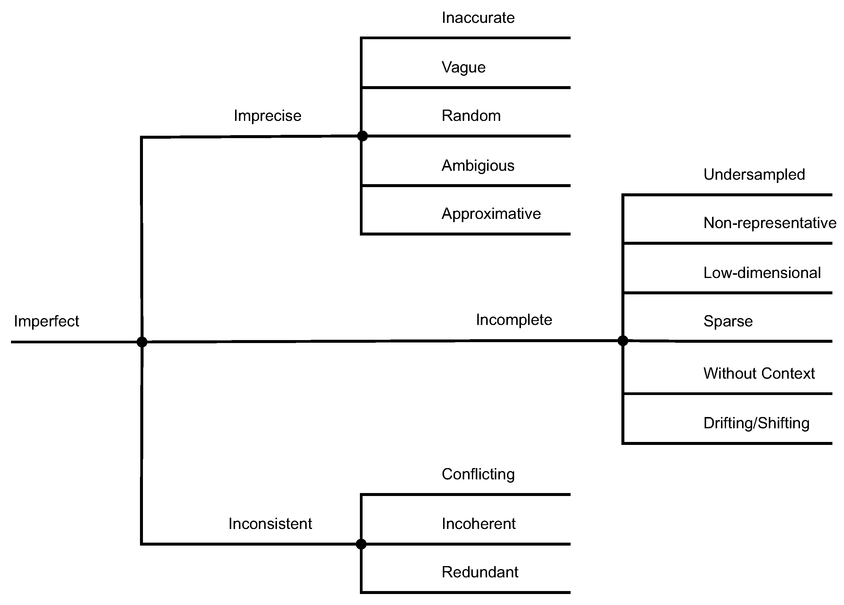
2. A Typology of Scarce Data

Scarce or incomplete data is a form of data imperfection that affects the ability of algorithms, machine-learned models, or human engineers to extract information and induce knowledge. Incomplete data represents uncertainty in the data, but also leads to uncertainty in the process of induction. In this sense, it is closely related to uncertainties—especially to the notion of epistemic uncertainty. It follows an introduction of epistemic uncertainty together with its counterpart aleatoric uncertainty.

Definition 1

(Aleatoric Uncertainty). Aleatoric uncertainty refers to the inherent variation of an object, concept, process, or phenomenon. It is random and non-deterministic in nature [15]. Even if data is complete and the underlying process is completely understood, the outcome of this process cannot be predicted with absolute certainty [16,17]. Consequently, gathering more data—or adding new data or information sources—does not reduce aleatoric uncertainty. Take, for example, a classification problem. In such a problem, aleatoric uncertainty is the intra-class distance or variance.

Definition 2

(Epistemic Uncertainty). In contrast, epistemic uncertainty results from a lack of knowledge about a phenomenon. This lack is caused by incomplete—not available—or inconsistent information. Epistemic uncertainty is, in principle, reducible by gathering additional information. In practice, reducing epistemic uncertainty is often not possible, feasible, or valuable [15,16,17]. In technical or industrial systems, this is due to one or more of the following reasons.

• Sensors are not available or limited in their functionality. They are technically infeasible, too costly, or not obtainable. The engineering effort to design and plan sensor systems is too complex or too expensive. The sensors’ properties are limited, for example, their sampling rate or operating range.
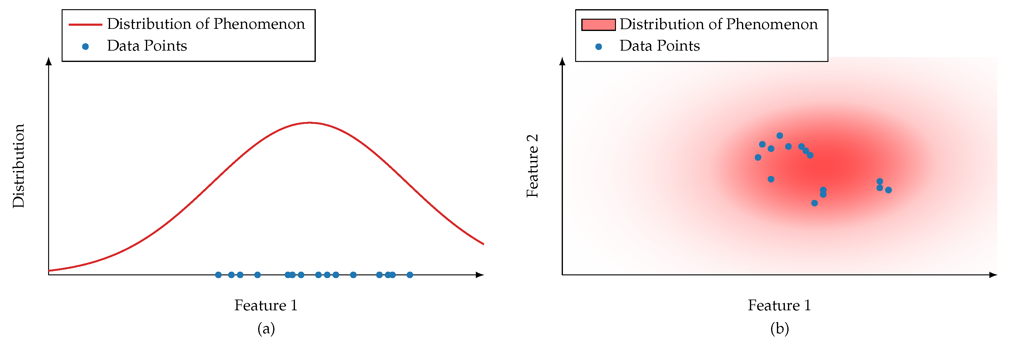
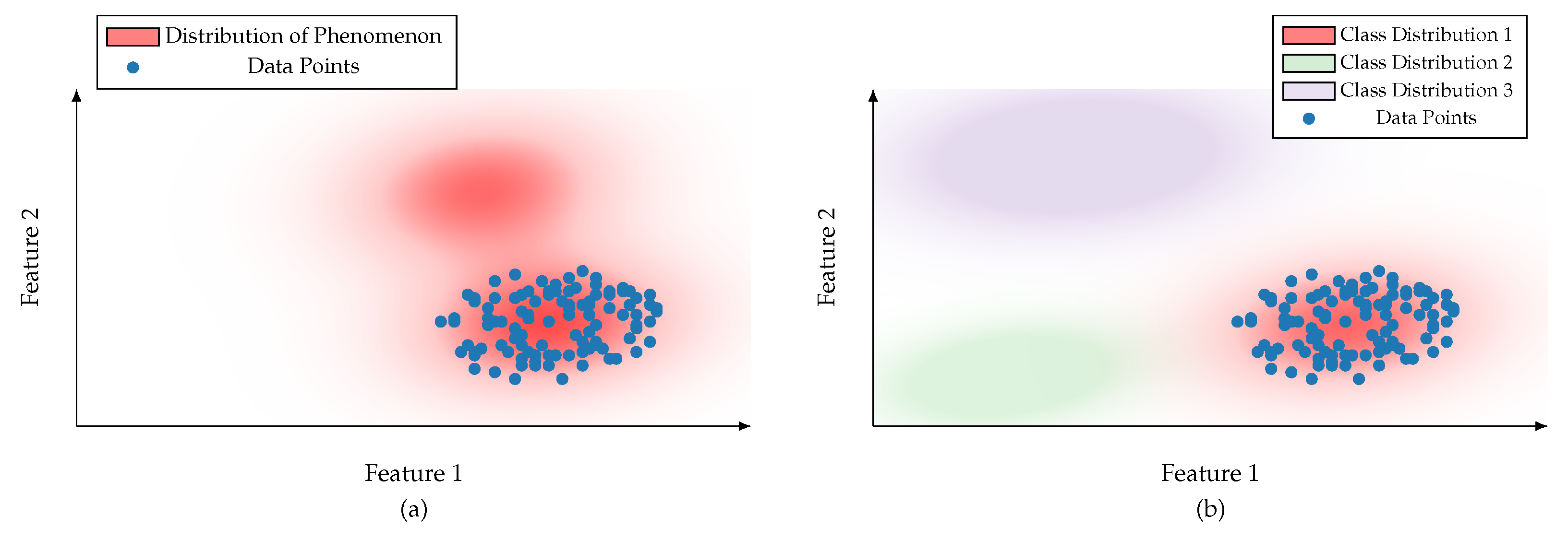
• The observation period or sampling size is insufficient. Observations do not cover certain concepts or phenomena (Data does not capture the Black Swan [18]). The operation of a sensor is too costly, takes too much time, or is destructive.
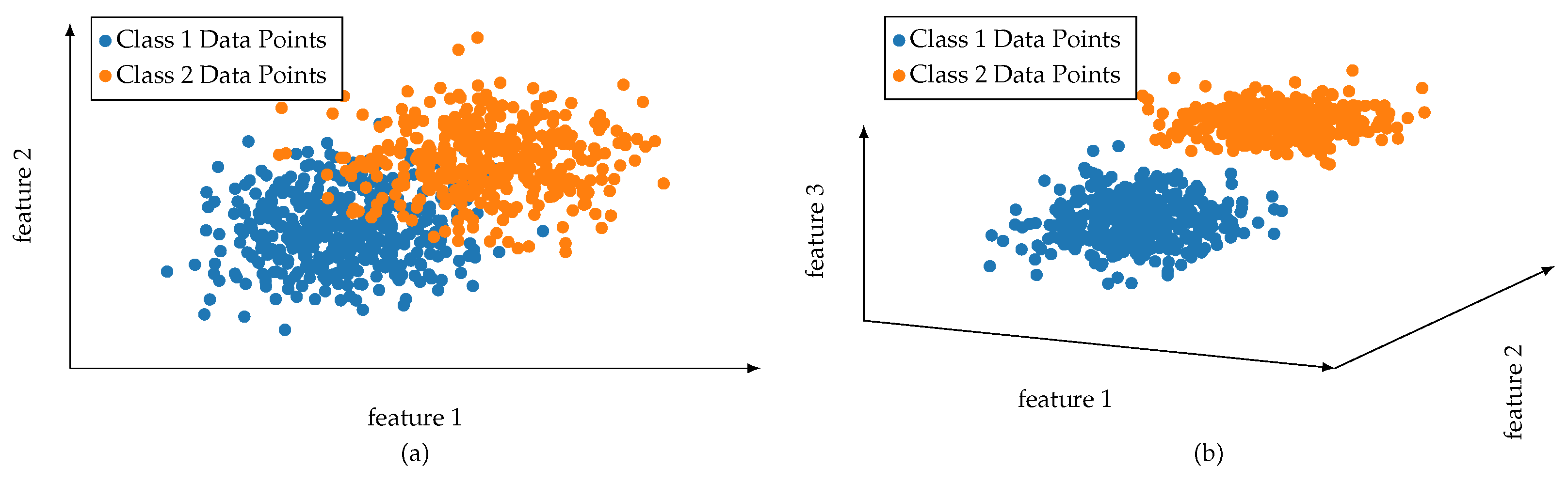
• Blind ignorance of human engineers prevents all potential data from being obtained. Missing knowledge about real-world phenomena or the availability of sensors limits the amount of data gathered.

Scarce Data is, therefore, itself a form of epistemic uncertainty. Handling epistemic uncertainty is one of the major challenges in data analysis. This is also recognised in machine learning research very recently [19,20,21]. To overcome this challenge, it is crucial to understand the various types of scarcity, their causes, and their interactions.

Several taxonomies and typologies have been proposed in the literature to categorise and relate data or information imperfections, uncertainties, and quality [15,22,23,24,25,26]. An overview of taxonomies and typologies is given by Jousselme et al. [27], which includes some of the works just mentioned. An overview of data quality in databases provided by de Almeida et al. [28] is also of interest. The authors identify data completeness as a major data quality issue. However, work limited to databases will not be discussed further here. Instead, we summarise taxonomies and typologies which focus on or at least address incompleteness, missing data, or missing information in

Table 1. Taxonomies of uncertainty, imperfection, ignorance, and quality which address the topic of data or information incompleteness (in the sense of missing data or information, i.e., scarcity). Incompleteness is recognised as the main concept of imperfection throughout the referenced works. However, a categorisation of the various kinds of missing data or information is not carried out.

Authors	Focus	Builds	Relies on	Details Subcategories of Incompleteness
		upon	Incompleteness
Smithson [22]	Ignorance	-	yes	Partially. Incompleteness is subcategorised into Uncertainty (including Vagueness, Probability, Ambiguity) and Absence. Absence of information is not further detailed.
Smets [23]	Imperfection	-	yes	No
Krause and Clark [29]	Uncertainty	-	yes	No
Ayyub and Klir [15]	Ignorance	[22]	yes	Partially. Similar to Smithson.
Bosu and MacDonell [24]	Data Quality	-	yes	No
Rogova [25]	Information Quality	[23]	yes	No
Raglin et al. [26]	Uncertainty	-	yes	No

. Most of the works referenced in Table 1 rely on the term incompleteness which is used interchangeably with scarcity in the table.

This survey shows that incompleteness is recognised broadly as a type of data imperfection, a kind of uncertainty, and a source of ignorance. In nearly all referenced taxonomies, incompleteness is not further subcategorised. A detailed look into various forms of incompleteness and missing data is not provided.

In the following, we present a more detailed typology of incompleteness as a form of imperfection (see Figure 1) based on Smets’ [23] taxonomy. This typology perceives incompleteness as a form of data imperfection along with imprecision and inconsistency.

The proposed typology subdivides incompleteness into six categories.

Undersampled: Data points always represent only a sample of a distribution or the characteristics of a phenomenon. Sensors only provide a window into the real world. Their observations are a fragmented representation. A phenomenon is undersampled if there is insufficient data available to make sound and significant findings about its characteristics. Due to undersampled data, information remains partially hidden. The aleatoric uncertainty of a phenomenon can only be described inadequately. Figure 2 illustrates two cases of undersampling using a scatter plot in a one-dimensional and a two-dimensional feature space.

As a consequence, training with machine learning methods does not lead to satisfactory results. The generalisation ability of the trained models is questionable at best. Probabilistic methods rely on the availability of statistically sound data or knowledge about prior distributions [30]. Kalman filters, for example, assume zero-mean Gaussian distributed data [31]. In the case of undersampled data, this knowledge cannot be derived from the data itself. Few data points also increase the risk of finding spurious correlations in the data [32]—especially when many features or data sources are involved. Another threat of undersampled data is that machine-learned models tend to easily overfit [33].

Non-representative: Data or information is non-representative when only certain parts or subconcepts of a phenomenon are observable or represented in the data. Other subconcepts may be very well represented. Take, for example, a bi-modal distribution of a phenomenon’s characteristics. One of the modes may be very well sampled, whereas the other is absent in the data. In extreme cases, complete concepts are missing. In less extreme cases, subconcepts may merely be undersampled. Data in which subconcepts are undersampled are often also referred to as biased. The observation of industrial machines (condition monitoring) often produces non-representative data. Machines are specifically built to run as smoothly and faultlessly as possible. Consequently, data obtained during normal operation is often available in abundance. In contrast, data on fault states or unusual operating conditions are often rare. Reducing this kind of epistemic uncertainty is difficult in practice since running a machine in fault states is either costly or infeasible. Figure 3 shows the multi-modal and condition monitoring examples as a form of non-representative data.

Low-dimensional: Real-world processes can only be observed by a finite number of sensors. Data may be incomplete due to missing data sources – in this case, the data space is too low-dimensional. A low-dimensional space may be insufficient to handle the aleatoric uncertainty of the phenomenon at hand. Figure 4 illustrates a case where data is scarce with respect to the number of available sources.

This epistemic uncertainty is reducible by adding new sources although it is crucial to carefully select new sources that are meaningful.

Sparse: Sparse data is caused by sensors or data sources which do not provide data continuously. For example, data is missing over certain time periods or data from different sources cannot be synchronised with each other. Missing data can be caused by defective sensors. This leads to data gaps. Take, for instance, data which is organised in a two-dimensional table. Its rows represent data instances and its columns are data sources. Sparse data is then characterised by missing entries throughout this table (think of a sparse matrix).

Without Context: Context is needed to extract information and knowledge from data. Roughly speaking, context is itself information that surrounds the phenomenon of interest and its data-generating process [34]. Context aids in understanding the phenomenon. It can be provided by domain knowledge. Examples of context are labels in classification applications or maps in applications of autonomous driving. Context, and specifically labels, are often costly to produce or provide. If in large datasets only a fraction of data instances are labelled, then the problem relates to undersampled data.

Drifting/Shifting: The effectiveness of machine learning algorithms relies heavily on the assumption that training and test data are taken from the same or at least similar distributions [35]. In reality, concepts and phenomena often drift in their distribution over time, e.g., data clusters move through feature space. As a consequence, models which have learned from training data are outdated as soon as significant drift occurs. Adaptation or retraining is usually necessary. Because the drifting data distribution over time is not known, drift is categorised as a form of incomplete information.

These six types of incomplete data have different causes, characteristics, and effects on machine learners or other data-processing algorithms. To overcome the associated challenges, algorithms have to specifically consider each type. This has to be kept in mind in designing data analyses.

3. An Overview of Methods for Working with Scarce Data

The challenges associated with scarce data have been known and intensively discussed in the research community for some time. Various methods and approaches exist that can deal with scarce data. In the following, we discuss methods of transfer learning, data augmentation, and information fusion that act in very different ways on scarce data. This survey is closely related to the work of Adadi [8], who studied machine learning methods for scarce data. We extend this survey with an insight into information fusion methods. We mainly focus on the problem of undersampled data and non-representative data. In the ensuing discussion, we motivate further research efforts on the combination of machine learning and information fusion methods.

3.1. Transfer Learning

Transfer learning is a machine learning method in which a model that has been trained in one domain is reused in a related domain. The model is not completely retrained but only adapted by post-training [36,37]. The purpose of transfer learning is to be able to use machine learners even with scarce data. Transfer learning requires a model which has learned as many basic concepts of a domain as possible. For example, these may be geometric shapes in image data, basic patterns such as a Mexican hat in time series, or basic pronunciations or sounds in human speech. Once basic concepts are known to a model, few training examples are required to adapt to a new domain—even zero-shot learning is possible under specific circumstances and depending on the application [38]. Most commonly neural networks and convolutional neural networks are used to transfer learning, but other machine learning methods have been adapted for transfer learning, such as Markov logic networks [39] and Bayesian networks [40]. Transfer learning has been applied to many domains. A survey on machine diagnostics in industrial applications is provided by Yao et al. [41].

Transfer learning comes with several drawbacks and pitfalls. Because a source model is required to know as many concepts as possible, large datasets and resources are necessary to train the source model in the first place. Such a model needs to be trained on a general dataset, which is at best not domain-specific. Secondly, the target domain is still characterised by scarce data. Therefore, some risks remain even if the transfer is learned. Models are still at risk to overfit or detect spurious correlations [37,42]. Finally, performance is affected negatively if the source and target domain do not cover the same concepts or focus on different concepts. This is referred to as negative transfer [43,44]. For example, recent studies have shown that models trained on the ImageNet (https://www.image-net.org/, accessed on 9 November 2022) dataset favour texture over shape [45]. Transferring these models into domains in which textural information is less important and objects are mostly defined by shape—such as object recognition of machinery parts, screws, or nuts [46,47,48]—will not result in optimal performance.

3.2. Data Augmentation

Data augmentation refers to methods that artificially increase the amount of available data. The aim is to facilitate machine learners to train on even small amounts of training data. Augmentation creates slightly modified copies of existing data or completely new synthetic data [49]. Data augmentation techniques have been successfully applied to image [49,50], text and natural language [51,52,53], and time series data [54]. Augmentation has a regularising effect on machine learning models, helps to reduce overfitting, and can improve the generalisability of models [50]. Industrial applications of data augmentation are, for example, given by Dekhtiar et al. [46], Židek et al. [47,48], Parente et al. [55], or Shi et al. [56].

Additional data instances are usually created by applying various transformations to data. In image datasets, these are, e.g., rotations, scaling, cropping, colour transformations, distortions, or erasing random parts of an image [50]. In natural language, parts of a text are randomly swapped, inserted, deleted, or replaced synonymously [52]. Time series transformations take place either in the time or frequency domain. These include cropping, slicing, jittering, or warping among others [54]. These transformations aim to teach a machine learner which information is important for defining a concept. For example, additional rotated images teach that rotation is not important to a concept or class. It is still the same class. By replacing the background in images, models learn to focus on objects in the foreground. Thus, augmenting data by selected transformations allows us to integrate expert knowledge into the machine learning process. However, it is crucial to apply the right transformation for a particular application in order for the data augmentation to be useful. Often data augmentation seems to be carried out in an “ad-hoc manner with little understanding of the underlying theoretical principles”—as stated by Dao et al. [57].

Another approach to data augmentation is to create additional data automatically by generative models such as generative adversarial networks [58]. The expectation is that expert’s knowledge will no longer be necessary or will be at least less crucial. A major drawback of generative augmentation is that it is susceptible to perpetrate bias in data [59].

With all these methods, there is a risk of losing important information in the augmentation process. Information may be discarded, e.g., by cropping an image, or may be overwritten by erasing parts of a text randomly [50,52]. It follows that patterns or classes are not correctly preserved. The data instance and its label may then no longer match (The label is not preserved). This problem is aggravated if small details in a data instance are crucial for a concept. Slight changes to the original data may then already be enough to distort or destroy concepts.

3.3. Information Fusion

Scarce data and epistemic uncertainty are intensively addressed in the research field of information fusion. Information fusion has been researched since the midst of the 20th century as a distinct field in parallel to machine learning [60,61]. While information fusion has similar goals and applications as machine learning—such as classification, regression, detection, or recognition—its focus differs. The aim of information fusion methods is to extract and condense high-quality information from a set of low-quality data sources [62]. Information fusion explicitly assumes that sources provide incomplete or imprecise information. The task of information fusion is to make the best of what imperfect data is available [14]. Fusion methods include a strong focus on modelling uncertain, error-prone, imprecise, and vague information [63]. For instance, fuzzy information is modelled via fuzzy set theory. Missing information or ignorance are modelled via evidence theories, such as the Dempster-Shafer theory. Fusion methods address scarce data with possibility theory. In direct comparison to probability theory, possibility theory is characterised by the fact that incomplete information is represented qualitatively [64]. The possibility theory requires a smaller amount of data but is less expressive in the final analysis [63,64]. Established methods of machine learning, on the other hand, rarely model missing information or epistemic uncertainty explicitly. Instead, they rely on a quantitative evaluation of data. In the following, we provide an overview of the mathematical tools fusion relies on, that is, the Dempster-Shafer theory, the fuzzy set theory, and the possibility theory.

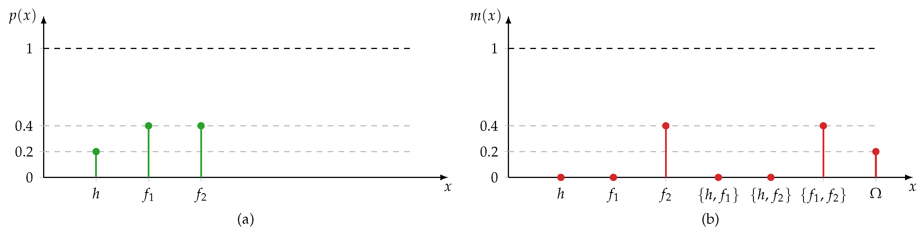
3.3.1. Dempster-Shafer Theory

The Dempster-Shafer theory of evidence (DST) has been proposed by Shafer [65] on the foundation of Dempster’s works on a framework for expressing upper and lower probabilities [66]. In the DST, available evidence forms the basis to express a degree of belief in a proposition that quantifies incomplete knowledge [67]. In this basic sense, it is comparable to Bayesian probability theory. It is motivated by the fact that probability theory is not able to distinguish between ignorance (epistemic uncertainty) and well-informed uncertainty (aleatoric uncertainty) natively [65].

Probability theory (ProbT) operates on a frame of discernment $\Omega$ which includes all given propositions or hypotheses X as singletons, i.e., $\Omega =\{X_1,X_2,\dots ,X_n\}$. Each proposition is given a probability $0\le p\left(x\right)\le 1$ to be true with the restriction of ${\sum }_{X\in \Omega }p\left(X\right)=1$. In the case of total ignorance, one tends to distribute probabilities uniformly over $\Omega$ but this is arbitrary. A uniform distribution is not distinguishable from a situation in which it is known that propositions are actually equally likely. DST allows us to assign evidence to sets of combined propositions. It operates on the power set of the frame of discernment, i.e., $\mathcal{P}\Omega =\{\varnothing ,X_1,X_2,\dots ,\{X_1,X_2\}\dots ,\Omega \}$. By assigning evidence m to combined propositions (e.g., $\{X_1,X_2\}$), a state of incomplete knowledge is expressed. In case of $\{X_1,X_2\}$, it is unclear whether evidence favours $X_1$ or $X_2$. Belief in a proposition is then obtained by $\mathrm{Bel}\left(X\right)={\sum }_{A\subseteq X}m\left(A\right)$. The usage of the power set allows DST to handle incomplete knowledge due to scarce data better and more properly than probability theory. An example of the difference between ProbT and DST is given in Figure 5.

DST is designed with a fusion of independent multiple sources in mind. Having multiple partially ignorant and uncertain sources, the aim is to get to a single estimation with reduced ignorance and increased certainty. To achieve this, most fusion rules involve a reinforcement effect. If, for example, $m_1\left(X\right)=m_2\left(X\right)$, then the fused mass $m_{12}\left(X\right)>m_1\left(X\right)$. Several fusion rules have been proposed over the years, for example, Dempster’s rule of combination [66,68], Yager’s rule [69], Campos’ rule [70], or the Balanced Two-Layer Conflict Solving rule [61], to name just a few.

DST fusion achieves that—if a group of sensors, experts, or machine learning models is uncertain in their assessments because of scarce data—to increase certainty. A popular approach in machine learning is to apply ensemble learners [71]. In ensemble learning, multiple weak learners are trained simultaneously. Their outputs are fused into a single one. An example of an ensemble is random forests. Although this seems to be an exemplary area of application for DST fusion, most ensemble learners rely on majority votings or averaging functions [72,73,74]. This motivates further research efforts in combining DST and machine learning methods as a way to handle the effects of scarce data.

3.3.2. Fuzzy Set Theory

Fuzzy set theory (FST) was proposed by Zadeh [75] motivated by the intrinsic vague nature of language. The fuzzy set theory facilitates the modelling of imprecise and vague information (cf. Figure 1). Although FST is not focused on incomplete information, it brings benefits when it comes to scarce data. Zadeh introduces sets with vague boundaries in contrast to crisp sets known from probability theory or Dempster-Shafer theory. In a crisp set, an element either belongs to this set or not. Its membership function $\mu$ is a mapping of all elements belonging to the frame of discernment $\Omega$ to a boolean membership $\mu :\Omega \to \{0,1\}$. Fuzzy sets allow degrees of memberships, that is, $\mu :\Omega \to [0,1]$.

The inherent vagueness of fuzzy membership functions can be exploited to learn class distributions from only a few data instances [76]. If class borders are only needed to be modelled imprecisely and vaguely, then less effort has to be put into a training process than learning precise class borders. The fuzzy membership of a data instance is then interpreted as the uncertainty of the classification model. This blurring of class borders results in weaker models with the upside of less data demand.

An approach for this kind of classification is fuzzy pattern classifiers (FPC). Fuzzy pattern classifiers have been introduced and advanced by Bocklisch [77,78]. An FPC learns a unimodal potential function for each data source. This function serves as a membership function. Each membership function is a weak classifier in itself. Seen as a group, the membership functions are similar to an ensemble. They output each a gradual estimate for the predicted membership. This allows to apply fuzzy aggregation rules to fuse the outputs into a singular class membership (see for example previous works by Holst and Lohweg [79,80,81,82]).

Unimodal potential functions were proposed by Aizerman et al. [83] as a pattern recognition tool. It was only later that they were applied as membership functions for fuzzy sets. Unimodal potential functions are used to model the distribution of compact and convex classes. Lohweg et al. [84] described a resource-efficient variant optimised for limited hardware:

$$\begin{array}{c}\mu \left(x\right)=\left\{\begin{array}{c}{2}^{-d(x,{\mathbf{p}}_{\mathrm{l}})}\mathrm{if}x\le \overline{x},\hfill \\ 2^{-d(x,{\mathbf{p}}_{\mathrm{r}})}\mathrm{if}x>\overline{x},\hfill \end{array}\right.\end{array}$$

$$\begin{array}{c}\mathrm{with}d(x,{\mathbf{p}}_{\mathrm{l}})={\left(\frac{\left|x-\overline{x}\right|}{C_{\mathrm{l}}}\right)}^{D_{\mathrm{l}}},\\ d(x,{\mathbf{p}}_{\mathrm{r}})={\left(\frac{\left|x-\overline{x}\right|}{C_{\mathrm{r}}}\right)}^{D_{\mathrm{r}}},\mathrm{and}\\ x \mathrm{a} \mathrm{data} \mathrm{instance} (\mathrm{measurement} \mathrm{value}).\end{array}$$

The unimodal potential function has several advantages for the use of scarce data. The function is parameterizable with few parameters. The number of parameters scales with data sources linearly. The parameters are relatively easy to train in data. Training methods can be found in [76,81,84]. The parameters are intuitive to interpret. Therefore, expert knowledge can be integrated easily. On the other hand, FPCs require unimodal and convex data distributions. In this regard, Hempel [85] proposed a multi-modal FPC, although his approach requires more training data in general.

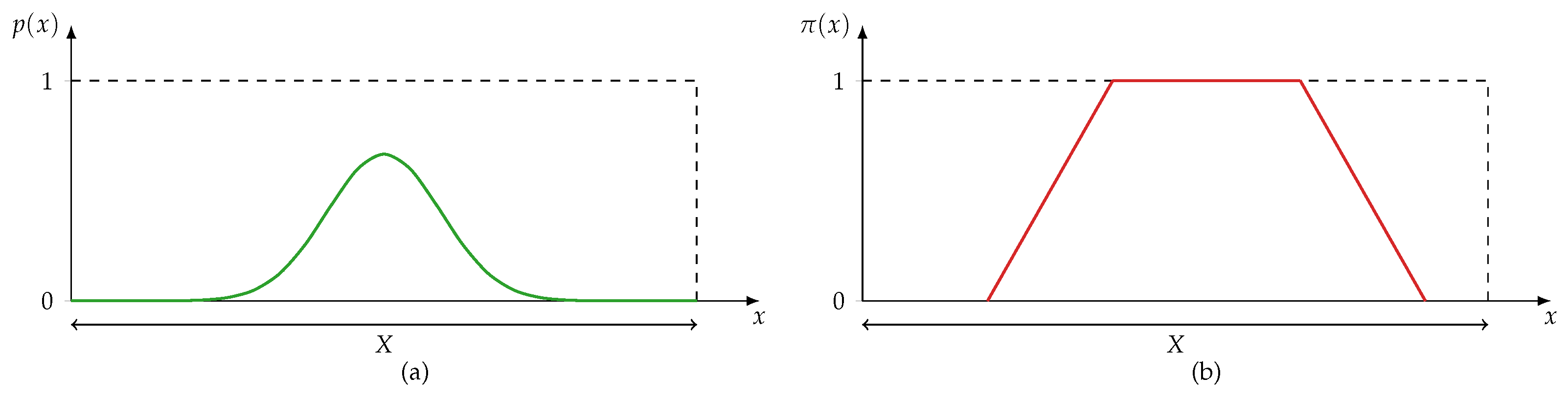
3.3.3. Possibility Theory

The possibility theory (PosT) was introduced by Zadeh in 1978 as an extension of fuzzy set theory [86]. It is designed as a counterpart to probability theory because of its limited ability to represent epistemic uncertainty.

Possibility theory is based on possibility distributions $\pi$—similar to probability distributions p. The possibility $0\le \pi \left(x\right)\le 1$ conveys how plausible the event x is. A value $\pi \left(x\right)=1$ means completely plausible; $\pi \left(x\right)=0$ completely implausible. At least one x is required to be fully plausible (normality requirement). But more than one x can be fully plausible. This leads to ${\sum }_{x\in \Omega }\pi \left(x\right)\ge 1$ or ${\int }_{x\in \Omega }\pi \left(x\right)\ge 1$.

Possibility distributions are similarly defined as fuzzy membership functions, that is, $\pi \left(x\right)=\mu \left(x\right)$ [16]. This has the advantage that mathematical operations defined on fuzzy sets can be directly applied to possibility distributions [87]. Though it has to be verified first if this is sensible. Fuzzy membership functions and possibility distributions differ in interpretation. Let x be an alternative for an unknown value v and A be a fuzzy set. The $\pi \left(x\right)$ expresses the possibility of $x=v$ knowing that $x\in A$. In contrast, $\mu \left(x\right)$ expresses the degree of membership of x to A knowing that $x=v$.

Possibility distributions are also a less expressive and weaker model than probability distributions. Roughly speaking, it is easier to conclude that a proposition is possible rather than probable. Moreover, for a proposition to be probable it must preliminarily be possible. This leads to the probability/possibility consistency principle stating that $\pi \left(x\right)\ge p\left(x\right)$. In return, possibility distributions require less effort – meaning training data or expert’s knowledge – to construct [88]. They do not require statistically sound data because they model incomplete information qualitatively; whereas probability distributions model random phenomena quantitatively. This distinction is highlighted in Figure 6.

This leads to the conclusion that possibility theory is well-suited to be used in the case of epistemic uncertainty and scarce data.

3.4. Discussion

Scarce data and epistemic uncertainty remain major challenges to machine learning and data analysis approaches. Missing information in data obstructs inherent aleatoric uncertainty.

In the area of machine learning, several techniques for coping with few training data have been thoroughly studied. Some of the most important are data augmentation, transfer learning, and interpretable models. While data augmentation and transfer learning focus on undersampled data mainly, interpretable models address also non-representative data. But only recently has epistemic uncertainty come into focus. Researchers have begun to explicitly define and quantify epistemic uncertainty of machine learning models [17,20,21,89].

In contrast, the research field of information fusion focuses on scarce data and epistemic uncertainty since its emergence in the mid-twentieth century. Fusion methods apply evidence theories such as DST, fuzzy set theory, and possibility theory to either quantify epistemic uncertainty or reduce its impact on performance.

However, combining fusion and machine learning methods is rare in the state of the art, although research need has been recognised recently [90,91,92]. Several works have been published that attempt to fill this open research topic. Among these are approaches which apply fusion techniques as a preprocessing step before machine learning [93,94]. These works focus on providing a machine learner with a more robust and condensed data basis through prior fusion. They do not focus on incomplete information though. Further works devise classifiers based on the Dempster-Shafer theory [95,96,97]. Finally, machine learning in a possibilistic setting exists but is very rare. A small survey is conducted by Dubois et al. [98]. This leads to the conclusion that further research is needed to more successfully and formally address scarce data in machine data analysis.

4. Conclusions

Despite the increasing number of sensors and measuring devices, data is often scarce in industrial applications. The scarcity of data stems from limited sensor availability and functionality, limited observation periods, hidden concepts, and the inevitable blind ignorance of engineers. This leads to challenges in data analysis. In this paper, we have typologized missing data and information in more detail based on the works of Smets [23]. According to this new typology, incomplete data is categorised into (1) undersampled, (2) non-representative, (3) low-dimensional, (4) sparse, (5) without context, and (6) drifting data. Existing typologies did not or only insufficiently detail the category of incompleteness [15,22,23,24,25,26,29]. In this respect, we have filled an open gap in existing works.

This paper also explored machine learning and information fusion methods that deal with scarce data and incomplete information. As such, this paper complements Adadi’s survey [8], which is limited to machine learning methods. Regarding machine learning, we focused on methods enabling data-hungry algorithms to be used on scarce data. Such methods are data augmentation [9] and transfer learning [10], among other methods. The idea behind transfer learning is to reuse and adapt models which have been trained on large, preferably general, datasets. However, efforts for training a source model are substantial and the risk of negative transfer has to be considered. Data augmentation creates new data points artificially by modifying existing ones. Data augmentation can reduce overfitting at the risk of destroying information.

Information fusion, on the other hand, relies on evidence theories, fuzzy set theory, and possibility theory to model, quantify, and cope with epistemic uncertainty [14]. This paper motivates and calls for further research efforts in combining fusion and machine learning approaches.

References

1. Sharp, M.; Ak, R.; Hedberg, T. A survey of the advancing use and development of machine learning in smart manufacturing. J. Manuf. Syst. 2018, 48, 170–179. [Google Scholar] [CrossRef] [PubMed]
2. Carvalho, T.P.; Soares, F.A.; Vita, R.; Francisco, R.D.P.; Basto, J.P.; Alcalá, S.G. A systematic literature review of machine learning methods applied to predictive maintenance. Comput. Ind. Eng. 2019, 137, 106024. [Google Scholar] [CrossRef]
3. Lei, Y.; Yang, B.; Jiang, X.; Jia, F.; Li, N.; Nandi, A.K. Applications of machine learning to machine fault diagnosis: A review and roadmap. Mech. Syst. Signal Process. 2020, 138, 106587. [Google Scholar] [CrossRef]
4. Babbar, R.; Schölkopf, B. Data scarcity, robustness and extreme multi-label classification. Mach. Learn. 2019, 108, 1329–1351. [Google Scholar] [CrossRef] [Green Version]
5. Wang, Q.; Farahat, A.; Gupta, C.; Zheng, S. Deep time series models for scarce data. Neurocomputing 2021, 456, 504–518. [Google Scholar] [CrossRef]
6. Shu, J.; Xu, Z.; Meng, D. Small Sample Learning in Big Data Era. arXiv 2018, arXiv:1808.04572. [Google Scholar]
7. Qi, G.J.; Luo, J. Small Data Challenges in Big Data Era: A Survey of Recent Progress on Unsupervised and Semi-Supervised Methods. IEEE Trans. Pattern Anal. Mach. Intell. 2022, 44, 2168–2187. [Google Scholar] [CrossRef]
8. Adadi, A. A survey on data–efficient algorithms in big data era. J. Big Data 2021, 8, 24. [Google Scholar] [CrossRef]
9. Andriyanov, N.A.; Andriyanov, D.A. The using of data augmentation in machine learning in image processing tasks in the face of data scarcity. J. Phys. Conf. Ser. 2020, 1661, 012018. [Google Scholar] [CrossRef]
10. Hutchinson, M.L.; Antono, E.; Gibbons, B.M.; Paradiso, S.; Ling, J.; Meredig, B. Overcoming data scarcity with transfer learning. arXiv 2017, arXiv:1711.05099. [Google Scholar]
11. Chen, Z.; Liu, Y.; Sun, H. Physics-informed learning of governing equations from scarce data. Nat. Commun. 2021, 12, 6136. [Google Scholar] [CrossRef] [PubMed]
12. Vecchi, E.; Pospíšil, L.; Albrecht, S.; O’Kane, T.J.; Horenko, I. eSPA+: Scalable Entropy-Optimal Machine Learning Classification for Small Data Problems. Neural Comput. 2022, 34, 1220–1255. [Google Scholar] [CrossRef] [PubMed]
13. Bhouri, M.A.; Perdikaris, P. Gaussian processes meet NeuralODEs: A Bayesian framework for learning the dynamics of partially observed systems from scarce and noisy data. Philos. Trans. R. Soc. A Math. Phys. Eng. Sci. 2022, 380, 20210201. [Google Scholar] [CrossRef]
14. Dubois, D.; Liu, W.; Ma, J.; Prade, H. The basic principles of uncertain information fusion. An organised review of merging rules in different representation frameworks. Inf. Fusion 2016, 32, 12–39. [Google Scholar] [CrossRef]
15. Ayyub, B.M.; Klir, G.J. Uncertainty Modeling and Analysis in Engineering and the Sciences; Chapman & Hall/CRC: Boca Raton, FL, USA, 2006. [Google Scholar]
16. Lohweg, V.; Voth, K.; Glock, S. A possibilistic framework for sensor fusion with monitoring of sensor reliability. In Sensor Fusion; Thomas, C., Ed.; IntechOpen: London, UK, 2011. [Google Scholar]
17. Hüllermeier, E.; Waegeman, W. Aleatoric and epistemic uncertainty in machine learning: An introduction to concepts and methods. Mach. Learn. 2021, 110, 457–506. [Google Scholar] [CrossRef]
18. Taleb, N.N. The Black Swan: The Impact of the Highly Improbable; Incerto, Random House Publishing Group: New York, NY, USA, 2007. [Google Scholar]
19. Abdar, M.; Pourpanah, F.; Hussain, S.; Rezazadegan, D.; Liu, L.; Ghavamzadeh, M.; Fieguth, P.; Cao, X.; Khosravi, A.; Acharya, U.R.; et al. A review of uncertainty quantification in deep learning: Techniques, applications and challenges. Inf. Fusion 2021, 76, 243–297. [Google Scholar] [CrossRef]
20. Huang, Z.; Lam, H.; Zhang, H. Quantifying Epistemic Uncertainty in Deep Learning. arXiv 2021, arXiv:2110.12122. [Google Scholar]
21. Bengs, V.; Hüllermeier, E.; Waegeman, W. Pitfalls of Epistemic Uncertainty Quantification through Loss Minimisation. arXiv 2022, arXiv:2203.06102. [Google Scholar]
22. Smithson, M. Ignorance and Uncertainty: Emerging Paradigms; Cognitive science; Springer: New York, NY, USA; Heidelberg, Germany, 1989. [Google Scholar]
23. Smets, P. Imperfect Information: Imprecision and Uncertainty. In Uncertainty Management in Information Systems: From Needs to Solutions; Motro, A., Smets, P., Eds.; Springer: New York, NY, USA, 1997; pp. 225–254. [Google Scholar]
24. Bosu, M.F.; MacDonell, S.G. A Taxonomy of Data Quality Challenges in Empirical Software Engineering. In Proceedings of the 2013 22nd Australian Software Engineering Conference, Melbourne, VIC, Australia, 4–7 June 2013; pp. 97–106. [Google Scholar]
25. Rogova, G.L. Information quality in fusion-driven human-machine environments. In Information Quality in Information Fusion and Decision Making; Bossé, É., Rogova, G.L., Eds.; Springer: Cham, Switzerland, 2019; pp. 3–29. [Google Scholar]
26. Raglin, A.; Emlet, A.; Caylor, J.; Richardson, J.; Mittrick, M.; Metu, S. Uncertainty of Information (UoI) Taxonomy Assessment Based on Experimental User Study Results; Human-Computer Interaction. Theoretical Approaches and Design, Methods; Kurosu, M., Ed.; Springer: Cham, Switzerland, 2022; pp. 290–301. [Google Scholar]
27. Jousselme, A.L.; Maupin, P.; Bosse, E. Uncertainty in a situation analysis perspective. In Proceedings of the Sixth International Conference of Information Fusion, Cairns, QSL, Australia, 8–11 July 2003; Volume 2, pp. 1207–1214. [Google Scholar]
28. de Almeida, W.G.; de Sousa, R.T.; de Deus, F.E.; Daniel Amvame Nze, G.; de Mendonça, F.L.L. Taxonomy of data quality problems in multidimensional Data Warehouse models. In Proceedings of the 2013 8th Iberian Conference on Information Systems and Technologies (CISTI), Lisbon, Portugal, 19–22 June 2013; pp. 1–7. [Google Scholar]
29. Krause, P.; Clark, D. Representing Uncertain Knowledge: An Artificial Intelligence Approach; Springer: Dordrecht, The Netherlands, 2012. [Google Scholar]
30. Huber, W.A. Ignorance Is Not Probability. Risk Anal. 2010, 30, 371–376. [Google Scholar] [CrossRef]
31. Kim, Y.; Bang, H. Introduction to Kalman Filter and Its Applications: 2. In Introduction and Implementations of the Kalman Filter; Govaers, F., Ed.; IntechOpen: London, UK, 2018. [Google Scholar]
32. Calude, C.; Longo, G. The deluge of spurious correlations in big data. Found. Sci. 2017, 22, 595–612. [Google Scholar] [CrossRef] [Green Version]
33. Horenko, I. On a Scalable Entropic Breaching of the Overfitting Barrier for Small Data Problems in Machine Learning. Neural Comput. 2020, 32, 1563–1579. [Google Scholar] [CrossRef] [PubMed]
34. Snidaro, L.; Herrero, J.G.; Llinas, J.; Blasch, E. Recent Trends in Context Exploitation for Information Fusion and AI. AI Mag. 2019, 40, 14–27. [Google Scholar] [CrossRef]
35. Gama, J.; Žliobaitė, I.; Bifet, A.; Pechenizkiy, M.; Bouchachia, A. A Survey on Concept Drift Adaptation. ACM Comput. Surv. 2014, 46, 44:1–44:37. [Google Scholar] [CrossRef]
36. Pan, S.J.; Yang, Q. A Survey on Transfer Learning. IEEE Trans. Knowl. Data Eng. 2010, 22, 1345–1359. [Google Scholar] [CrossRef]
37. Weiss, K.; Khoshgoftaar, T.M.; Wang, D. A survey of transfer learning. J. Big Data 2016, 3, 9. [Google Scholar] [CrossRef] [Green Version]
38. Oreshkin, B.N.; Carpov, D.; Chapados, N.; Bengio, Y. Meta-learning framework with applications to zero-shot time-series forecasting. arXiv 2020, arXiv:2002.02887. [Google Scholar] [CrossRef]
39. Mihalkova, L.; Huynh, T.N.; Mooney, R.J. Mapping and Revising Markov Logic Networks for Transfer Learning; AAAI: Menlo Park, CA, USA, 2007. [Google Scholar]
40. Niculescu-Mizil, A.; Caruana, R. Inductive Transfer for Bayesian Network Structure Learning. In Proceedings of the Eleventh International Conference on Artificial Intelligence and Statistics, San Juan, Puerto Rico, 21–24 March 2007; Meila, M., Shen, X., Eds.; PMLR Proceedings of Machine Learning Research: New York City, NY, USA, 2007; Volume 2, pp. 339–346. [Google Scholar]
41. Yao, S.; Kang, Q.; Zhou, M.; Rawa, M.J.; Abusorrah, A. A survey of transfer learning for machinery diagnostics and prognostics. Artif. Intell. Rev. 2022. [Google Scholar] [CrossRef]
42. Sun, Q.; Liu, Y.; Chua, T.S.; Schiele, B. Meta-Transfer Learning for Few-Shot Learning. In Proceedings of the IEEE/CVF Conference on Computer Vision and Pattern Recognition (CVPR), Long Beach, CA, USA, 15–20 June 2019. [Google Scholar]
43. Wang, Z.; Dai, Z.; Poczos, B.; Carbonell, J. Characterizing and Avoiding Negative Transfer. In Proceedings of the IEEE/CVF Conference on Computer Vision and Pattern Recognition (CVPR), Long Beach, CA, USA, 15–20 June 2019. [Google Scholar]
44. Zhang, W.; Deng, L.; Zhang, L.; Wu, D. A Survey on Negative Transfer. IEEE/CAA J. Autom. Sin. 2022, 9, 1. [Google Scholar] [CrossRef]
45. Geirhos, R.; Rubisch, P.; Michaelis, C.; Bethge, M.; Wichmann, F.A.; Brendel, W. ImageNet-trained CNNs are biased towards texture; increasing shape bias improves accuracy and robustness. In Proceedings of the International Conference on Learning Representations, New Orleans, LA, USA, 6–9 May 2019. [Google Scholar]
46. Dekhtiar, J.; Durupt, A.; Bricogne, M.; Eynard, B.; Rowson, H.; Kiritsis, D. Deep learning for big data applications in CAD and PLM – Research review, opportunities and case study. Emerg. Ict Concepts Smart Safe Sustain. Ind. Syst. 2018, 100, 227–243. [Google Scholar] [CrossRef]
47. Židek, K.; Lazorík, P.; Piteľ, J.; Hošovský, A. An Automated Training of Deep Learning Networks by 3D Virtual Models for Object Recognition. Symmetry 2019, 11, 496. [Google Scholar] [CrossRef] [Green Version]
48. Židek, K.; Lazorík, P.; Piteľ, J.; Pavlenko, I.; Hošovský, A. Automated Training of Convolutional Networks by Virtual 3D Models for Parts Recognition in Assembly Process. In ADVANCES IN MANUFACTURING; Trojanowska, J., Ciszak, O., Machado, J.M., Pavlenko, I., Eds.; Lecture Notes in Mechanical Engineering; Springer: Cham, Switzerland, 2019; Volume 13, pp. 287–297. [Google Scholar]
49. Perez, L.; Wang, J. The effectiveness of data augmentation in image classification using deep learning. arXiv 2017, arXiv:1712.04621. [Google Scholar]
50. Shorten, C.; Khoshgoftaar, T.M. A survey on Image Data Augmentation for Deep Learning. J. Big Data 2019, 6, 60. [Google Scholar] [CrossRef]
51. Feng, S.Y.; Gangal, V.; Wei, J.; Chandar, S.; Vosoughi, S.; Mitamura, T.; Hovy, E. A Survey of Data Augmentation Approaches for NLP. arXiv 2021, arXiv:2105.03075. [Google Scholar]
52. Shorten, C.; Khoshgoftaar, T.M.; Furht, B. Text Data Augmentation for Deep Learning. J. Big Data 2021, 8, 101. [Google Scholar] [CrossRef] [PubMed]
53. Bayer, M.; Kaufhold, M.A.; Reuter, C. A Survey on Data Augmentation for Text Classification. ACM Computing Surveys 2022, accept. [Google Scholar] [CrossRef]
54. Wen, Q.; Sun, L.; Yang, F.; Song, X.; Gao, J.; Wang, X.; Xu, H. Time Series Data Augmentation for Deep Learning: A Survey. In Proceedings of the Thirtieth International Joint Conference on Artificial Intelligence, Virtual, 19–27 August 2021; International Joint Conferences on Artificial Intelligence Organization: Menlo Park, CA, USA, 2021. [Google Scholar]
55. Parente, A.P.; de Souza Jr, M.B.; Valdman, A.; Mattos Folly, R.O. Data Augmentation Applied to Machine Learning-Based Monitoring of a Pulp and Paper Process. Processes 2019, 7, 958. [Google Scholar] [CrossRef]
56. Shi, D.; Ye, Y.; Gillwald, M.; Hecht, M. Robustness enhancement of machine fault diagnostic models for railway applications through data augmentation. Mech. Syst. Signal Process. 2022, 164, 108217. [Google Scholar] [CrossRef]
57. Dao, T.; Gu, A.; Ratner, A.J.; Smith, V.; de Sa, C.; Ré, C. A Kernel Theory of Modern Data Augmentation. arXiv 2018, arXiv:1803.06084. [Google Scholar]
58. Antoniou, A.; Storkey, A.; Edwards, H. Data Augmentation Generative Adversarial Networks. arXiv 2017, arXiv:1711.04340. [Google Scholar]
59. Jain, N.; Manikonda, L.; Hernandez, A.O.; Sengupta, S.; Kambhampati, S. Imagining an Engineer: On GAN-Based Data Augmentation Perpetuating Biases. arXiv 2018, arXiv:1811.03751. [Google Scholar]
60. Hall, D.; Llinas, J. Multisensor Data Fusion. In Handbook of Multisensor Data Fusion; Electrical Engineering & Applied Signal Processing Series; Hall, D., Llinas, J., Eds.; CRC Press: Boca Raton, FL, USA, 2001; Volume 3. [Google Scholar]
61. Mönks, U. Information Fusion Under Consideration of Conflicting Input Signals; Technologies for Intelligent Automation; Springer: Berlin/Heidelberg, Germany, 2017. [Google Scholar]
62. Bloch, I.; Hunter, A.; Appriou, A.; Ayoun, A.; Benferhat, S.; Besnard, P.; Cholvy, L.; Cooke, R.; Cuppens, F.; Dubois, D.; et al. Fusion: General concepts and characteristics. Int. J. Intell. Syst. 2001, 16, 1107–1134. [Google Scholar] [CrossRef] [Green Version]
63. Dubois, D.; Everaere, P.; Konieczny, S.; Papini, O. Main issues in belief revision, belief merging and information fusion. In A Guided Tour of Artificial Intelligence Research: Volume I: Knowledge Representation, Reasoning and Learning; Marquis, P., Papini, O., Prade, H., Eds.; Springer: Cham, Switzerland, 2020; pp. 441–485. [Google Scholar]
64. Denœux, T.; Dubois, D.; Prade, H. Representations of uncertainty in artificial intelligence: Probability and possibility. In A Guided Tour of Artificial Intelligence Research: Volume I: Knowledge Representation, Reasoning and Learning; Marquis, P., Papini, O., Prade, H., Eds.; Springer: Cham, Switzerland, 2020; pp. 69–117. [Google Scholar]
65. Shafer, G. A Mathematical Theory of Evidence; Princeton University Press: Princeton, NJ, USA, 1976. [Google Scholar]
66. Dempster, A.P. Upper and lower probabilities induced by a multivalued mapping. Ann. Math. Stat. 1967, 38, 325–339. [Google Scholar] [CrossRef]
67. Salicone, S.; Prioli, M. Measuring Uncertainty within the Theory of Evidence; Springer Series in Measurement Science and Technology; Springer: Cham, Switzerland, 2018. [Google Scholar]
68. Shafer, G. Dempster’s rule of combination. Int. J. Approx. Reason. 2016, 79, 26–40. [Google Scholar] [CrossRef]
69. Yager, R.R. On the dempster-shafer framework and new combination rules. Inf. Sci. 1987, 41, 93–137. [Google Scholar] [CrossRef]
70. Campos, F. Decision Making in Uncertain Situations: An Extension to the Mathematical Theory of Evidence. Ph.D. Thesis, Dissertation.Com., Boca Raton, FL, USA, 2006. [Google Scholar]
71. Polikar, R. Ensemble Learning. In Ensemble Machine Learning: Methods and Applications; Zhang, C., Ma, Y., Eds.; Springer: New York, NY, USA, 2012; pp. 1–34. [Google Scholar]
72. Sagi, O.; Rokach, L. Ensemble learning: A survey. WIREs Data Min. Knowl. Discov. 2018, 8, e1249. [Google Scholar] [CrossRef]
73. Dong, X.; Yu, Z.; Cao, W.; Shi, Y.; Ma, Q. A survey on ensemble learning. Front. Comput. Sci. 2020, 14, 241–258. [Google Scholar] [CrossRef]
74. Zhou, Z.H. Ensemble Learning. In Machine Learning; Springer: Singapore, 2021; pp. 181–210. [Google Scholar]
75. Zadeh, L.A. Fuzzy sets. Inf. Control 1965, 8, 338–353. [Google Scholar] [CrossRef] [Green Version]
76. Mönks, U.; Petker, D.; Lohweg, V. Fuzzy-Pattern-Classifier training with small data sets. Information Processing and Management of Uncertainty in Knowledge-Based Systems. Theory and Methods; Hüllermeier, E., Kruse, R., Hoffmann, F., Eds.; Springer: Berlin/Heidelberg, Germany, 2010; pp. 426–435. [Google Scholar]
77. Bocklisch, S.F. Prozeßanalyse mit unscharfen Verfahren, 1st ed.; Verlag Technik: Berlin, Germany, 1987. [Google Scholar]
78. Bocklisch, S.F.; Bitterlich, N. Fuzzy Pattern Classification—Methodology and Application—. In Fuzzy-Systems in Computer Science; Kruse, R., Gebhardt, J., Palm, R., Eds.; Vieweg+Teubner Verlag: Wiesbaden, Germany, 1994; pp. 295–301. [Google Scholar]
79. Holst, C.A.; Lohweg, V. A conflict-based drift detection and adaptation approach for multisensor information fusion. In Proceedings of the 2018 IEEE 23rd International Conference on Emerging Technologies and Factory Automation (ETFA), Torino, Italy, 1–4 September 2018; pp. 967–974. [Google Scholar]
80. Holst, C.A.; Lohweg, V. Improving majority-guided fuzzy information fusion for Industry 4.0 condition monitoring. In Proceedings of the 2019 22nd International Conference on Information Fusion (FUSION), IEEE, Ottawa, ON, Canada, 2–5 July 2019. [Google Scholar]
81. Holst, C.A.; Lohweg, V. A redundancy metric set within possibility theory for multi-sensor systems. Sensors 2021, 21, 2508. [Google Scholar] [CrossRef]
82. Holst, C.A.; Lohweg, V. Designing Possibilistic Information Fusion—The Importance of Associativity, Consistency, and Redundancy. Metrology 2022, 2, 180–215. [Google Scholar] [CrossRef]
83. Aizerman, M.A.; Braverman, E.M.; Rozonoer, L.I. Theoretical foundations of the potential function method in pattern recognition learning. Autom. Remote Control 1964, 25, 821–837. [Google Scholar]
84. Lohweg, V.; Diederichs, C.; Müller, D. Algorithms for hardware-based pattern recognition. EURASIP J. Appl. Signal Process. 2004, 2004, 1912–1920. [Google Scholar] [CrossRef] [Green Version]
85. Hempel, A.J. Netzorientierte Fuzzy-Pattern-Klassifikation nichtkonvexer Objektmengenmorphologien. Ph.D. Thesis, Technische Universität Chemnitz, Chemnitz, Germany, 2011. [Google Scholar]
86. Zadeh, L.A. Fuzzy sets as a basis for a theory of possibility. Fuzzy Sets Syst. 1978, 1, 3–28. [Google Scholar] [CrossRef]
87. Solaiman, B.; Bossé, É. Possibility Theory for the Design of Information Fusion Systems; Information Fusion and Data Science; Springer: Cham, Switzerland, 2019. [Google Scholar]
88. Dubois, D.; Prade, H. Practical methods for constructing possibility distributions. Int. J. Intell. Syst. 2016, 31, 215–239. [Google Scholar] [CrossRef] [Green Version]
89. Wang, G.; Li, W.; Aertsen, M.; Deprest, J.; Ourselin, S.; Vercauteren, T. Aleatoric uncertainty estimation with test-time augmentation for medical image segmentation with convolutional neural networks. Neurocomputing 2019, 338, 34–45. [Google Scholar] [CrossRef]
90. Diez-Olivan, A.; Del Ser, J.; Galar, D.; Sierra, B. Data fusion and machine learning for industrial prognosis: Trends and perspectives towards Industry 4.0. Inf. Fusion 2019, 50, 92–111. [Google Scholar] [CrossRef]
91. Blasch, E.; Sullivan, N.; Chen, G.; Chen, Y.; Shen, D.; Yu, W.; Chen, H.M. Data fusion information group (DFIG) model meets AI+ML. In Signal Processing, Sensor/Information Fusion, and Target Recognition XXXI; Kadar, I., Blasch, E.P., Grewe, L.L., Eds.; SPIE: Bellingham, WA, USA, 2022; Volume 12122, p. 121220N. [Google Scholar]
92. Holzinger, A.; Dehmer, M.; Emmert-Streib, F.; Cucchiara, R.; Augenstein, I.; Del Ser, J.; Samek, W.; Jurisica, I.; Díaz-Rodríguez, N. Information fusion as an integrative cross-cutting enabler to achieve robust, explainable, and trustworthy medical artificial intelligence. Inf. Fusion 2022, 79, 263–278. [Google Scholar] [CrossRef]
93. Holst, C.A.; Lohweg, V. Feature fusion to increase the robustness of machine learners in industrial environments. at-Automatisierungstechnik 2019, 67, 853–865. [Google Scholar] [CrossRef]
94. Kondo, R.E.; de Lima, E.D.D.; Freitas Rocha Loures, E.D.; Santos, E.A.P.D.; Deschamps, F. Data Fusion for Industry 4.0: General Concepts and Applications. In Proceedings of the 25th International Joint Conference on Industrial Engineering and Operations Management—IJCIEOM, Novi Sad, Serbia, 15–17 July 2019; Anisic, Z., Lalic, B., Gracanin, D., Eds.; Springer International Publishing: Cham, Switzerland, 2020; pp. 362–373. [Google Scholar]
95. Denœux, T.; Masson, M.H. Dempster-Shafer Reasoning in Large Partially Ordered Sets: Applications in Machine Learning. In Integrated Uncertainty Management and Applications; Huynh, V.N., Nakamori, Y., Lawry, J., Inuiguchi, M., Eds.; Springer: Berlin/Heidelberg, Germany, 2010; pp. 39–54. [Google Scholar]
96. Hui, K.H.; Ooi, C.S.; Lim, M.H.; Leong, M.S. A hybrid artificial neural network with Dempster-Shafer theory for automated bearing fault diagnosis. J. Vibroengineering 2016, 18, 4409–4418. [Google Scholar] [CrossRef] [Green Version]
97. Peñafiel, S.; Baloian, N.; Sanson, H.; Pino, J.A. Applying Dempster–Shafer theory for developing a flexible, accurate and interpretable classifier. Expert Syst. Appl. 2020, 148, 113262. [Google Scholar] [CrossRef]
98. Dubois, D.; Prade, H. From possibilistic rule-based systems to machine learning—A discussion paper. In Scalable Uncertainty Management; Davis, J., Tabia, K., Eds.; Springer International Publishing: Cham, Switzerland, 2020; pp. 35–51. [Google Scholar]
Figure 1. A typology of data and information imperfection with a detailed subcategorisation of incompleteness. The typology is based on the work of Smets’ [23]. It recognises incompleteness as one of three major sources of imperfection – besides inconsistency and imprecision. Imprecision captures deficiencies that prevent unambiguous statements from being made based on individual data points. Inconsistency refers to situations in which a piece of information is contradictory to existing knowledge or with other information sources. Incompleteness is lacking, absent, or non-complete data and information.
Sci 04 00049 g001
Figure 2. Two examples showcasing undersampled data: (a) an ill-represented one-dimensional distribution and (b) an ill-represented two-dimensional distribution. A two-dimensional scatter plot showcasing undersampled data. The plots show the distributions of phenomena in feature space (red). The distributions are unknown and represent the aleatoric uncertainty of the phenomena. In both examples, the sampled data points (blue) are insufficient to draw conclusions about the distributions. The missing data points are a form of epistemic uncertainty.
Sci 04 00049 g002
Figure 3. Two cases of non-representative data. In (a) a bi-modal distribution is shown (red, unknown). One mode is very-well sampled; the second is missing in the data. Plot (b) shows a multi-class classification problem, in which certain classes are missing in the data. Such missing data can, for example, be due to unseen fault states of a machine.
Sci 04 00049 g003
Figure 4. A classification example in which the addition of a new data source allows us to distinguish two classes perfectly (b). In the two-dimensional space shown in (a), the aleatoric uncertainty prevents a clear separation of classes. Low-dimensional data is still a form of epistemic uncertainty as it is unknown how the class distributions evolve with new sources.
Sci 04 00049 g004
Figure 5. Probability theory versus Dempster-Shafer’s theory in a condition monitoring example. The basic propositions are h: the monitored object is healthy and f 1 , f 2 : the object is in one of two fault states. The distribution modelled with ProbT (a) is ambiguous since it cannot distinguish between ignorance (epistemic uncertainty) and well-informed uncertainty (aleatoric uncertainty). Using DST (b), it turns out that the expert or model is indeed partly ignorant. This is expressed by m ( { f 1 , f 2 } ) = 0.4 (a fault occurred but it is unknown which one) and by m ( Ω ) = 0.2 (nothing is known).
Sci 04 00049 g005
Figure 6. A continuous probability (a) and a continuous possibility distribution (b). The probability distribution models a random phenomenon quantitatively; the possibility of distribution of incomplete information qualitatively. The following applies: x Ω p ( x ) = 1 , x Ω π ( x ) 1 , and π ( x ) p ( x ) .
Sci 04 00049 g006