Article

Quantification and Reduction of Uncertainty in Seismic Resilience Assessment for a Roadway Network

1
Department of Civil & Environmental Engineering, Washington State University, Pullman, WA 99164, USA
2
Verisk Extreme Event Solutions, Boston, MA 02111, USA
3
Department of Civil & Environmental Engineering, Rowan University, Glassboro, NJ 08028, USA
*
Author to whom correspondence should be addressed.
Infrastructures 2023, 8(9), 128; https://doi.org/10.3390/infrastructures8090128
Submission received: 25 May 2023 / Revised: 11 August 2023 / Accepted: 16 August 2023 / Published: 25 August 2023

Abstract

:
The nation’s transportation systems are complex and are some of the highest valued and largest public assets in the United States. As a result of repeated natural hazards and their significant impact on transportation functionality and the socioeconomic health of communities, transportation resilience has gained increasing attention in recent years. Previous studies on transportation resilience have heavily emphasized network functionality during and/or following a scenario hazard event by implicitly assuming that sufficient knowledge of structural capacity and environmental/service conditions is available at the time of an extreme event. However, such assumptions often fail to consider uncertainties that arise when an extreme hazard event occurs in the future. Thus, it is essential to quantify and reduce uncertainties to better prepare for extreme events and accurately assess transportation resilience. To this end, this paper proposes a dynamic Bayesian network-based resilience assessment model for a large-scale roadway network that can explicitly quantify uncertainties in all phases of the assessment and investigate the role of inspection and monitoring programs in uncertainty reduction. Specifically, the significance of data reliability is investigated through a sensitivity analysis, where various sets of data having different reliabilities are used in updating system resilience. To evaluate the effectiveness of the model, a benchmark problem involving a highway network in South Carolina, USA is utilized, showcasing the systematic quantification and reduction of uncertainties in the proposed model. The benchmark problem result shows that incorporating monitoring and inspection data on important variables could improve the accuracy of predicting the seismic resilience of the network. It also suggests the need to consider equipment reliability when designing monitoring and inspection programs. With the recent development of a wide range of monitoring and inspection techniques, including nondestructive testing, health monitoring equipment, satellite imagery, LiDAR, etc., these findings can be useful in assisting transportation managers in identifying necessary equipment reliability levels and prioritizing inspection and monitoring efforts.

1. Introduction

Decisions aimed at ensuring the adequate performance and operational integrity of transportation systems have strong implications for the health and economic wellbeing of the communities that they serve. Since their disruptions would have detrimental effects on the continuous flow of people, essential goods, and vehicles, and, in turn, economic security, transportation systems are generally expected to maintain prescribed minimum levels of service under normal and even disturbed conditions. Specifically, during and following man-made and natural hazards (e.g., bomb blasts, explosions, earthquakes, hurricanes, and wildfires), transportation systems play a key role in providing access to the affected regions, enabling search and rescue, and transporting essential supplies [1].
Due to the frequent occurrences and grave consequences of natural disasters observed in recent years, research pertaining to the resilience assessment of transportation systems has received a great deal of attention. Resilience for an engineered system is generally defined as its capacity to withstand, adapt to, and recover rapidly from disruptions to ensure its performance and meet customer demand [2,3,4,5,6,7]. Since there has been no widely accepted measure of resilience for transportation systems, researchers have proposed to define and quantify such resilience in different manners. These metrics are generally divided into topological metrics [8], attributes-based metrics [9], and performance-based metrics [2]. However, many resilience metrics have focused on a snapshot of system resilience after the realization of a specific scenario hazard event, ignoring uncertainties in this scenario event as well as system resilience.
While uncertainty quantification and reduction in transportation resilience assessment are essential to ensuring cost-effective resilience-enhancing strategies, many studies that propose a new resilience metric or resilience-based decision framework do not investigate the role of inspection/monitoring programs. One reason for this is that most metrics or frameworks measure scenario-based static resilience assuming that, at the time of hazard event occurrence, the full probabilistic descriptions of structural capacity and external loadings are known. However, there are substantial uncertainties in (a) the number and time of hazard event occurrence, (b) structural capacity in the future, and (c) external/service loadings especially when climate change affects the performance of an asset or when traffic demands change significantly as a result of population growth and urbanization. In recent years, transportation agencies have also realized the increasing uncertainties arising from aging and deteriorating infrastructure, increasing complexity of networks, extreme events from natural and man-made hazards, budgets and resources, and increasing operational demands, among others. Failure to account for these factors and the associated uncertainties may affect the agency’s capability to achieve its predefined goals and objectives. Moreover, if a resilience-based decision framework extends to a specified period of time and is intended to capture the time-dependent changes in structural performance and resilience, inspection/monitoring programs are necessary to increase the reliability of our prediction about structural capacity and/or external loadings in the future and, ultimately, transportation-system resilience.
This paper proposes a dynamic Bayesian network (BN)-based seismic resilience assessment model for a large-scale roadway network that can explicitly quantify uncertainties in all phases of the assessment and investigate the role of inspection and monitoring programs in uncertainty reduction. First, uncertainties in transportation-system capacity and demand are identified and reduced through a dynamic BN based on measurement data collected over time. Then, the updated system capacity and demand are incorporated into network analysis to assess roadway resilience over time. Specifically, the role of measurement data in reducing uncertainty is investigated through a sensitivity analysis, where various sets of data having different reliability are used in updating system resilience. Finally, the proposed model is demonstrated with a benchmark problem, a highway network in South Carolina, to showcase how the model can systematically quantify and reduce uncertainties in assessing the seismic resilience of the highway network.

2. Literature Review

2.1. Transportation Resilience Assessment

Due to the unprecedented nature of disasters and their massive consequences, the resilience of a transportation system has been extensively studied in the literature on various modes of transportation, such as waterways, roadways, airways, and railways. As this paper develops a dynamic BN-based resilience assessment model for a large-scale roadway network, this section places more emphasis on the literature review of the resilience of a highway road network.
Many quantitative and qualitative methods have been developed in recent years to assess roadway-network resilience. For example, Adams et al. [10] proposed a set of criteria to qualitatively evaluate resilience when a road system was subjected to disruptive weather events. However, quantitative methods have been more prevalent in transportation engineering because of their ability to be coupled with transportation simulation and to provide a quantitative basis for effective decision-making. Quantitative transportation resilience metrics can be measured by simulation models, data-driven models, optimization models, or probabilistic models. Specifically, optimization models are useful for solving traffic-assignment problems and for optimizing preparedness and recovery activities/resources.
Murray-Tuite [9] is considered one of the first attempts to specifically define and quantitatively assess resilience in the context of transportation systems [1]. Murray-Tuite [9] stated that the use of multiple metrics and simulation techniques could provide a promising approach to addressing the complexity of resilience and defined ten dimensions of transportation resilience. To measure transportation resilience, Murray-Tuite [9] evaluated only four out of the ten dimensions, which were adaptability, safety, mobility, and recovery, by using the traffic assignment simulation methodology DYNASMART-P. Ip and Wang [11] utilized the weighted average number of reliable independent paths in the road network to quantitatively measure the resilience of transportation networks. Cox et al. [12] provided operational metrics to evaluate different aspects of transportation-system resilience (e.g., vulnerability, flexibility, and resource availability) under terrorist attacks. With an emphasis on enhancing the resilience of a transportation network, Liao et al. [13] aimed to measure and optimize transportation resilience under disasters. They considered three performance measurements (i.e., coping capacity, robustness, and flexibility) in evaluating transportation resilience.
To study network topological characteristics and their role in transportation resilience, Zhang et al. [14] proposed an optimization-based framework that considered throughput and connectivity in quantifying resilience and conducted numerical experiments on 17 different network structures by including preparedness and recovery activities. The results provided a basis for characterizing highly resilient network topologies and identifying network attributes that might lead to poorly performing systems. Ganin et al. [15] stated that evaluating road networks based only on their operating state during normal conditions resulted in little information about system performance under disrupted conditions. By using observed data of annual delay per peak-period auto commuter, they developed an urban roadway-efficiency model and used it to calculate resilience. They defined resilience as a change in efficiency resulting from roadway disruptions and applied their model to road transportation networks in 40 major US cities. The results showed that, under disruptive conditions, the failure of network components ultimately led to the failure of the entire network and suggested that it would be important to evaluate the significance of network components in prioritizing network resilience improvement activities.
However, most of the previous studies on transportation resilience have focused on the effect of a scenario hazard event on system performance in the immediate aftermath of such an event and provided a snapshot of system resilience. While some existing studies have considered uncertainties in this scenario event as well as system resistance [16,17], uncertainties have not been explicitly characterized, tracked, or reduced in the process. Moreover, the role of inspection/monitoring programs and data reliability in uncertainty reduction has not yet been studied in existing transportation resilience literature.

2.2. Use of Bayesian Network in Transportation Risk and Resilience Assessment

In the process of resilience evaluation, there are substantial uncertainties involved as much information is not available regarding disruptive events. Moreover, these events occur sometime far in the future. Some recent studies have attempted to account for uncertainties in transportation resilience assessment using various models, such as the Markov chain [18,19], neural network [20], and diffusion graph convolutional network [21]. However, thus far, BN is one of the most widely adopted models for addressing uncertainties due to its conceptual clarity, flexibility, and sequential learning capability. BN is a graphical model that permits the design of stochastic relationships among a group of variables, thereby allowing a clear framework for incorporating new data into existing knowledge. Moreover, due to its flexibility, BN can handle a wide range of data types, including discrete, continuous, subjective, and mixed data. Additionally, BN inherently enables sequential learning, which is suitable particularly when sequential data are involved.
John et al. [22] presented a resilience assessment approach that employed BN to model various influencing variables in a seaport system. The study showed that the proposed methodology could provide safety analysts with a useful tool to implement resilience-enhancing strategies for maritime systems. Hosseini and Barker [23] offered a methodology to quantify resilience as a function of absorptive, adaptive, and restorative capacities using BNs. BN was used in their study to track and quantify uncertainty propagation and, ultimately, improve resilience-enhancing decision-making. They applied their model to an inland waterway network and demonstrated how sensitivity analyses could improve pre- and post-disaster strategies for building system resilience. Castillo et al. [24] presented a BN-based model for the probabilistic risk assessment of railway lines. In their model, they attempted to reduce the complexity of the problem because railway lines in the real world have variables as high as thousands or more. To achieve this goal, they divided the BN into small parts such that the complexity of the problem would become linear in the number of items and subnetworks. Additionally, the application of the backward inference process of BN helped identify the causes when an accident occurred.
While transportation resilience is often dynamic due to the evolving nature of external and internal factors affecting transportation performance, most of the abovementioned studies have considered resilience as a static one and employed static BN. Kammouh et al. [25] presented both static and dynamic BN frameworks to evaluate the resilience of engineering systems. The dynamic BN extends the classical BN by adding a time dimension. The proposed resilience framework was presented in the form of a mathematical formulation that integrated the probability distributions of all variable states. The static BN framework was applied to evaluate the resilience of the country of Brazil against natural and manmade disasters, while the dynamic BN framework was used to evaluate the resilience of a transportation system. Their study showed that the dynamic BN framework performed better in dynamically modeling complex systems, even in cases where data were scarce.
In summary, BN has been used extensively in the literature to assess the risk and resilience of complex engineering systems due to its ability to represent conditional dependencies between a set of variables. Specifically, the aspects of BN, like the forward and backward propagation, have been highly successful in decision-making in the face of uncertainty.

2.3. Summary

From the literature review, most of the studies on transportation resilience have thoroughly emphasized network functionality during or following a scenario hazard event by implicitly assuming that sufficient knowledge of structural capacity and environmental/service conditions is available at the time of an extreme event. However, it is identified that such knowledge often involves uncertainties and, thus, uncertainties should be quantified and properly managed to improve the accuracy of resilience assessment. Moreover, only a few studies have considered the interdependencies between random variables in the assessment model. One way of addressing this issue is to embed dynamic BN in the resilience assessment model to quantify uncertainties in major random variables that may affect the resilience capacities of transportation systems not only at the present time but also in the future. Furthermore, it is important to include the effect of monitoring and inspection activities throughout the lifecycle of transportation systems, aiming at reducing uncertainties and improving the accuracy of resilience assessment. To address the research gaps identified in this section, we propose a transportation resilience assessment model, where dynamic BN and information entropy are used to quantify and reduce uncertainties in resilience-related random variables while formulating interdependencies between these variables.

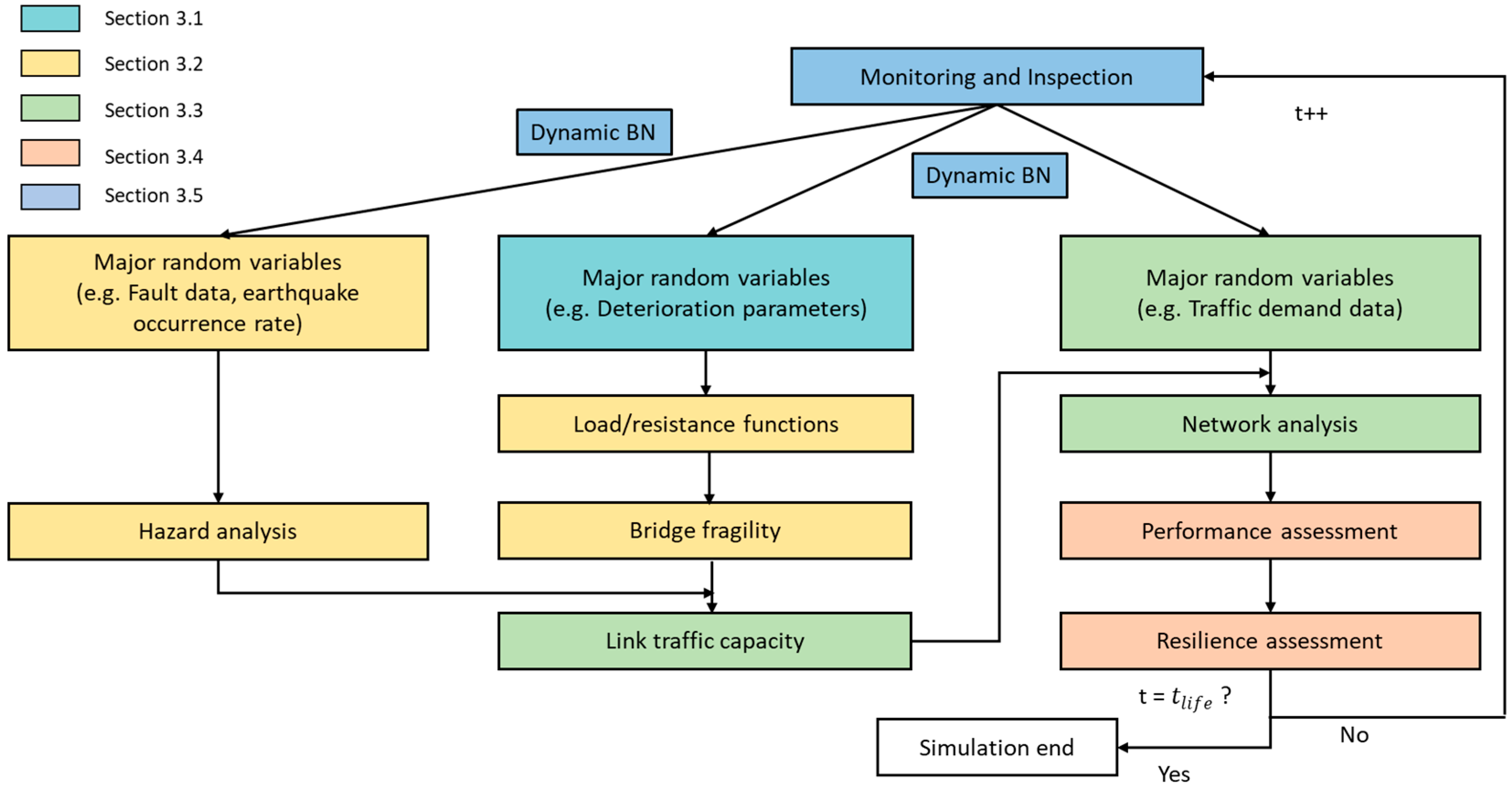
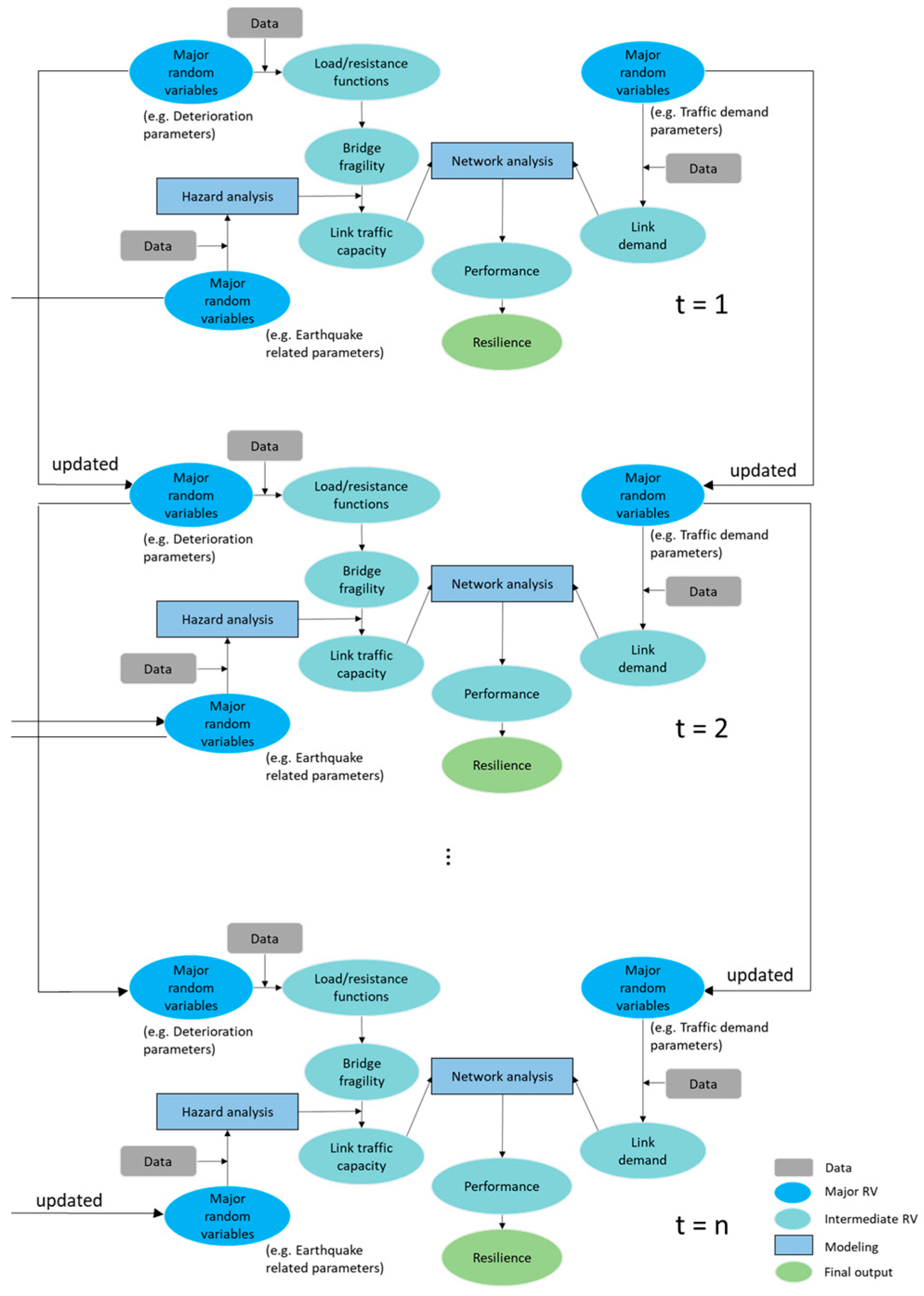
3. Methodology: Dynamic BN-Based Seismic Resilience Assessment Model

This section proposes a model that quantifies and reduces uncertainties along the process of seismic resilience assessment through information entropy and dynamic BN. Figure 1 shows the overall flowchart of the proposed dynamic BN-based seismic resilience assessment of a highway network. As illustrated in Figure 1, the model begins by measuring the time-dependent structural vulnerability of individual bridges exposed to corrosion (Section 3.1) and linking this measure to post-earthquake traffic carrying capacity (Section 3.2). Then, the performance of individual bridges is aggregated through network analysis to evaluate the performance of the highway network in terms of total travel time prior to and following a hazard event (Section 3.3). By incorporating time-dependent restorative activities into the network analysis, the network seismic resilience is assessed (Section 3.4). In the meantime, the probability density functions (PDFs) of bridge and network functionalities are updated based on inspection and monitoring data over time through dynamic BN (Section 3.5). Finally, information entropy is used to quantify uncertainties in the seismic resilience index and to study the sensitivity of seismic resilience to the reliability of inspection and monitoring data (Section 3.5).

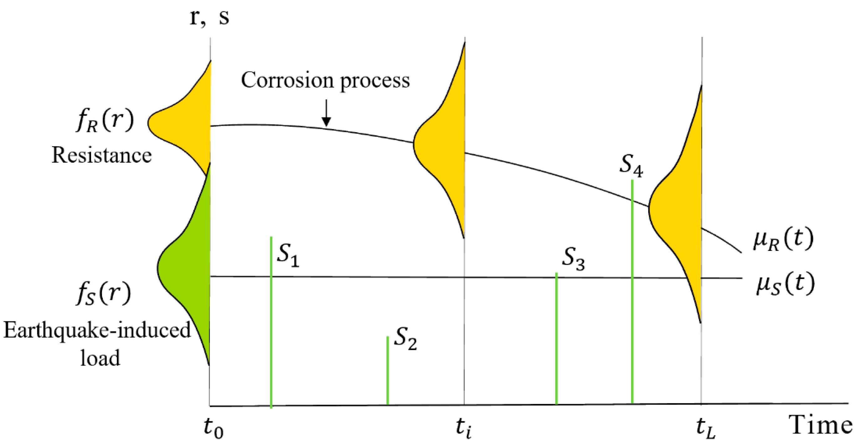
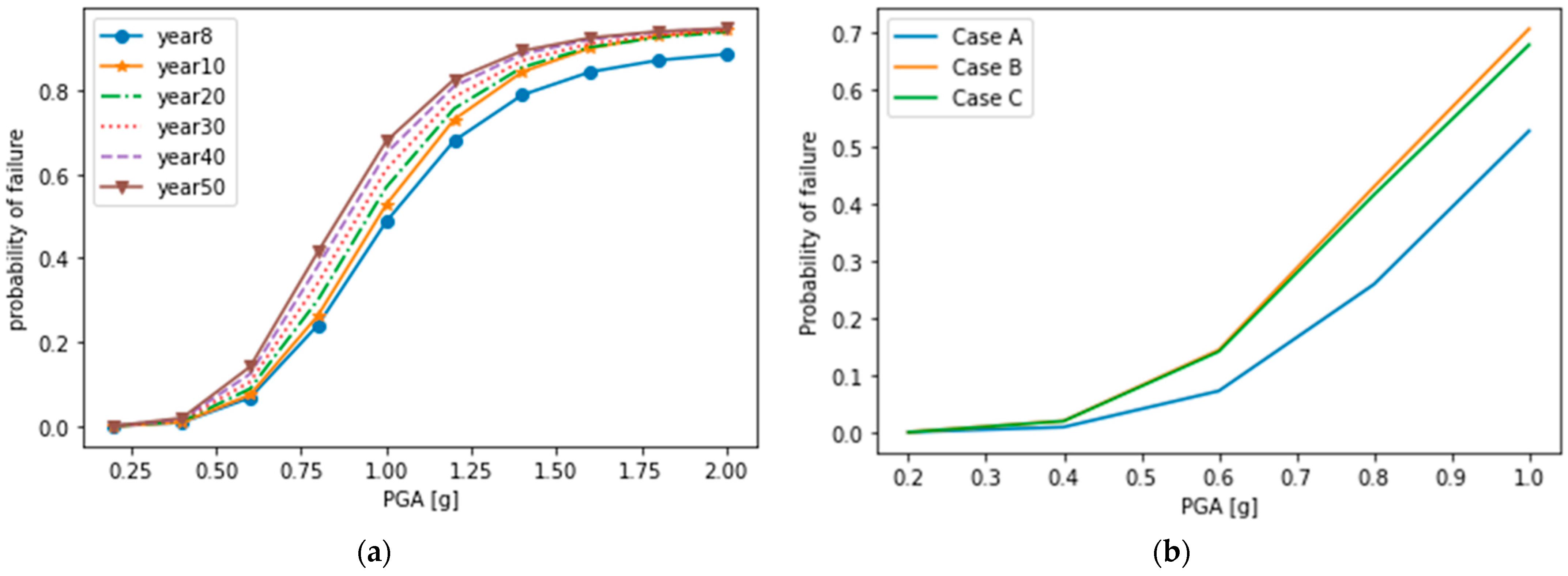
3.1. Time-Dependent Structural Reliability Assessment of Bridges Exposed to Corrosion

Bridges are one of the most critical elements in a transportation network; based on past experiences (e.g., the 1994 Northridge earthquake, the 1995 Kobe earthquake, the 1999 Chi-Chi earthquake, the 2011 Tohoku earthquake, etc.), they are perceived as one of the most vulnerable components that may experience significant structural damage in the event of an earthquake [26,27,28,29]. While it is essential to consider other factors contributing to the overall performance of transportation networks during earthquake events, such as roadway and pavement damage, tunnel damage, landslides, etc., this study is specifically focused on the analysis of the post-earthquake performance of individual bridges especially when they are exposed to corrosion.
Bridges in coastal environments or cold climates are exposed to chloride-induced corrosion, which is known to be a major cause of structural deterioration. As shown in Figure 2, a bridge slowly loses its capacity to resist extreme loading over time due to corrosion and, therefore, has a higher probability of failure when being subjected to earthquakes. Time-dependent reliability (i.e., the probability that the limit state of a bridge will not be exceeded) is modeled by incorporating time-dependent deterioration in the structural elements.
For a reinforced concrete (RC) member, chloride accumulation profiles in concrete can be modeled by using Fick’s second law [30,31,32]:
C x , t = C s 1 e r f x 2 D c t
where C ( x ,   t ) = the chloride concentration at a distance x (m) from the surface at time t ; C s = the chloride concentration at the surface (kg/m3); e r f = the gaussian error function; and D c = the diffusion coefficient (m2/year). By setting C ( x ,   t ) equal to the critical chloride concentration ( C c r ), Equation (1) can be solved for t . Then, the corresponding corrosion initiation time, T i , is calculated by [33]:
T i = x 2 4 D c e r f 1 C s C c r C s 2
Once corrosion initiates, the reinforcement diameter decreases over time and can be mathematically expressed by a time-dependent function:
D t = D 0 r c o r r t T i
where D t = the reinforcement diameter at time t ;   D 0 = the initial diameter of a reinforcing rebar; and r c o r r = the rate of corrosion. Consequently, the remaining cross-sectional area of reinforcement can be estimated by the following expressions [34]:
A t =             n D 0 2 π 4                                                                                               f o r   t     T i n [ D t ] 2 π 4                 f o r   T i < t < T i + D i / r c o r r 0                                                                                           f o r   t T i + D i r c o r r
in which n = the number of reinforcing rebars.
The failure probability of the bridge structure is computed, as expressed by Equation (5):
P f ( t ) = 0 0 s f R , S t d r d s
where P f ( t ) = the failure probability of a component or system; and f R , S t = the joint probability distribution of resistance ( R ) and load ( S ) functions. Since structural deterioration due to corrosion reduces the strength of a component or system over time, the time-dependent failure probability will be estimated by accounting for the effects of corrosion deterioration in the resistance model.
In this paper, we adopt the parameterized seismic fragility model proposed by Ghosh [35] to assess the time-dependent failure probability of a bridge. It is because (a) this model can reduce substantial computation burden by replacing a large number of nonlinear dynamic analyses of complete finite element models with a surrogate model [36]; (b) it can capture time-dependent deterioration in the structural elements; and (c) it can incorporate new observed data obtained from field-measurement instrumentation and update the failure probability of the bridge. The parameterized fragility curve equation is generally expressed by [36]:
P s y s | i m , x 1 , x 2 ,   ,   x m = P b i n s y s ,   i   = 1 i m , x 1 , x 2 , ,   x m = e θ s y s , 0 + θ s y s , i m i m + j = 1 m θ s y s ,   j   x j 1 + e θ s y s , 0 + θ s y s , i m + j = 1 m θ s y s , j x j
in which P s y s | i m , x 1 , x 2 ,   ,   x m = the conditional probability of system-level failure; i m = the intensity of ground motions; x = the set of m critical parameters affecting the seismic performance of the deteriorating bridge; b i n = the binary vector indicating either system survival ( b i n = 0) or system failure ( b i n = 1); and θ = the set of logistic regression coefficients. To reduce uncertainties involved in the structural deterioration process, the deterioration parameters (e.g., C s , D c , and r c o r r ) can be monitored through field instrumentation and used to update the input vector x through BN. Ultimately, the updated input vectors are incorporated into the parameterized fragility curve to update the probability of failure. This procedure will be illustrated in more detail in Section 3.5.

3.2. Post-Earthquake Traffic Flow Capacity Assessment of Highway Bridges

Following an earthquake event, a bridge can be fully operational or can carry only some portion of the traffic load that can be safely carried by an intact bridge. Truck weight and speed restrictions or lane closures can be implemented to reduce the traffic load that needs to be carried by a damaged bridge. To assess the post-earthquake functionality of a bridge, in this subsection, we adopt a methodology for linking the post-earthquake reliability index of a bridge to the resulting traffic flow capacity by adjusting the mean values of live load in a reliability calculation [37]. Using this relationship, the post-earthquake reliability index obtained from Section 3.1 can be used to find the associated allowable traffic flow capacity.
In Section 3.1, the probability of failure of an individual bridge given a specific ground-motion intensity can be calculated by Equation (6). Then, the reliability index, β , of a bridge structure is calculated by:
β = Φ 1 1 p f
where Φ 1 ( · ) = the inverse of the cumulative distribution function of a standard normal random variable; and p f = the probability of failure of the bridge. The relationship between β and traffic flow capacity is developed based on the working-backward method [37]. The detailed procedure for developing the relationship between the post-earthquake reliability index and traffic carrying capacity can be found in Ghasemi and Lee [37].

3.3. Network Analysis: A Highway Network Involving Multiple Bridges

Network analysis is a computational framework used to evaluate network-level performance by accounting for the interactions between various components. The performance of a network can be evaluated in terms of total travel time. Conventional connectivity often accounts only for two binary states of a link (full capacity or complete failure), which may mislead the actual performance of the network. On the other hand, travel time and costs can consider different levels of link capacities and incorporate dynamic traffic demand over time. Thus, travel time and cost are useful measures to determine network performance under traffic flow variation [38] and to be used in a cost–benefit analysis to determine the effectiveness of institutional investments in maintenance and repair activities in improving the resilience of a road network.
In this paper, we assess highway-network performance using the CUBE voyager software program which enables macroscopic traffic simulation. It is a transportation planning software commonly used in evaluating the performance of transportation networks, analyzing travel demand, and estimating travel time. This program requires network GIS data, the traffic capacity and demand at each link, and origin–destination (O-D) pairs as major input data. During normal operations, the performance of the highway network is assessed by the aggregated travel time of the fastest routes between all O-D pairs. Following an earthquake event, post-earthquake link capacities obtained from Section 3.2 are incorporated into the network analysis to determine the fastest routes between the same set of O-D pairs. The performance of the highway network is assessed at every time interval whenever new information on major random variables becomes available.

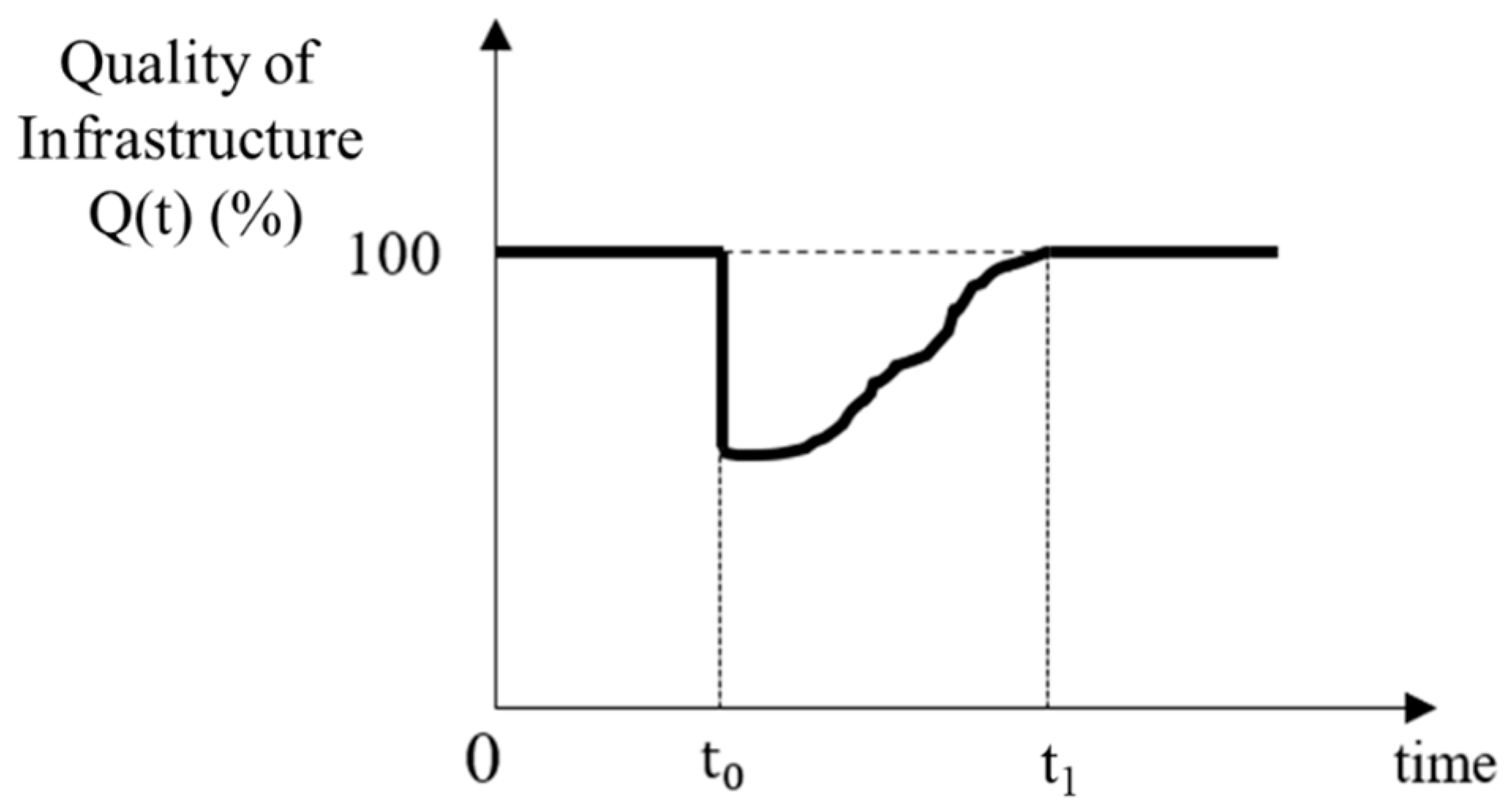
3.4. Seismic Resilience Assessment of a Highway Network

This subsection illustrates the procedure for assessing the seismic resilience of a highway network. Although there is no single agreed upon indicator for measuring resilience, loss of resilience, R l o s s , with respect to a specific earthquake event, has been widely used as a resilience indicator over the past two decades [2]. As shown in Figure 3, the loss of resilience can be measured by the area above the post-earthquake recovery trajectories and accounts for both the expected degradation in quality and the recovery time. It is mathematically expressed by:
R l o s s = t 0 t 1 100 Q t d t
where t 0 = the time of occurrence of an earthquake event; t 1 = the time when a bridge/network is completely repaired; and Q ( t ) = the time-dependent quality (or performance) of the structure. To improve the seismic resilience of the structure, R l o s s should be reduced.
A similar formulation is adopted in this study. The seismic resilience of a highway network is measured by the normalized area under the post-earthquake recovery trajectories and can be expressed as:
R = 1 t 1 t 0 t 0 t 1 Q t d t
Contrary to R l o s s , a higher value of R indicates a more seismically resilient network. In this paper, network performance is expressed as a function of total travel time as follows [39]:
Q t = 100 100 T T T t T T T 0 T T T 0
where T T T t = the total travel time at time t ; and T T T 0 = the total travel time in the base model (measured without any disaster event).
To capture both the time-dependent nature of resilience and uncertainty propagation, network resilience is assessed at every time step (e.g., 2 years) over a specified time period (e.g., 50 years) by assuming that a highway network is subjected to the same scenario earthquake event. Network resilience is expected to change due to time-dependent bridge reliability and traffic demand. However, due to substantial uncertainties in seismic resilience assessment, the estimated network resilience could be different from true network resilience. Thus, inspection and monitoring activities are performed continuously over time and their measurement results are incorporated in updating the stochastic models of bridge fragility and link traffic demand through dynamic BN. Using the updated models, network resilience is estimated at every time step and is compared with the one estimated based only on prior information to investigate the role of inspection/monitoring programs in reducing uncertainties in seismic resilience assessment.

3.5. Uncertainty Quantification and Propagation in Resilience Assessment

This subsection illustrates the procedure for quantifying uncertainties and tracking their propagation from individual stochastic models to overall resilience assessment. There are two types of uncertainties—aleatory and epistemic. Aleatory uncertainties are defined as randomness or the inherent variability of a physical phenomenon and, thus, are essentially irreducible. For example, wind speeds at a site are typically characterized by Weibull distribution. Additional sampling will not change its coefficient of variation in any significant way. On the other hand, epistemic uncertainties are knowledge based and generally can be reduced with additional knowledge. Additional knowledge comes at a price and there is a trade-off between cost and uncertainty reduction. Thus, in this study, epistemic uncertainties are reduced by incorporating additional information obtained from inspection and field instrumentation through BN.
BN has been widely applied in the field of reliability and resilience assessment due to its ability to update prior knowledge based on newly observed data. BN is a reliable tool that accounts for the influence of uncertainty and variability to predict model outcomes for a complex system. In Bayes’ Theorem, initial knowledge of a parameter ( θ ) is encoded in a prior PDF, f θ . After incorporating observed data ( d ), a posterior PDF of the parameter, f θ | d , is calculated by:
f θ | d = f d | θ f θ f d
where f d | θ = the likelihood function that quantifies the likelihood of observing this data given θ ; and f d = the marginal probability of the data. As such, the posterior PDF of the parameter is obtained by updating the prior PDF in light of the observed data and is more informative than the prior one.
As shown in Figure 4, major random variables related to corrosion, seismic hazards, and traffic demands can be monitored. Additional nodes can be introduced into the existing Bayesian network (i.e., Figure 4) to account for other random variables and uncertain factors that could potentially affect network performance. In the proposed resilience assessment framework, the parameterized fragility curve equations (c.f., Equation (6)) of individual bridges are continually updated based on field instrumentation data, while traffic-count data, such as annual average daily traffic (AADT) data, are incorporated to update the prior PDF of traffic demand on each link. BN can be used to develop a series of probabilistic graphical models aimed at identifying the relative contributions of uncertainties at each stage to uncertainties in the overall resilience.
Information entropy is used to quantify uncertainties in the PDFs of random variables in resilience assessment. Specifically, in this paper, information entropy is used to quantitatively assess the effect of data reliability (or accuracy) on the reduction of uncertainties. In classical physics, entropy is a measure of the quantity of energy that is no longer available to do physical work. Shannon [40] extended the entropy concept to information theory to quantify the amount of information as follows:
I x i = log p i
where I ( · ) = the amount of information; X = the random variable; and P = the probability distribution of X . The value I ( · ) indicates how much information there is in a random variable X . For example, an event having a lower probability has more information than common events and, thus, has a higher value of I . On the other hand, there is no information content in a certain or deterministic event. The information entropy, which is also called Shannon entropy, is the expected amount of information in a random variable and is calculated by the following equation [41]:
H x = E I X
The information entropy for a discrete random variable X is expressed by:
H x = i = 1 n p i   I x i = i = 1 n p i log p i    
Similarly, the information entropy for a continuous random variable X is defined as:
H x = f x log f x d x

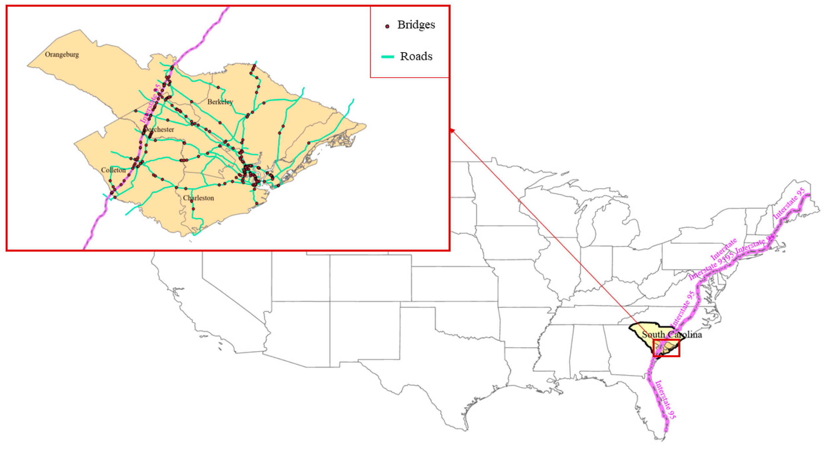
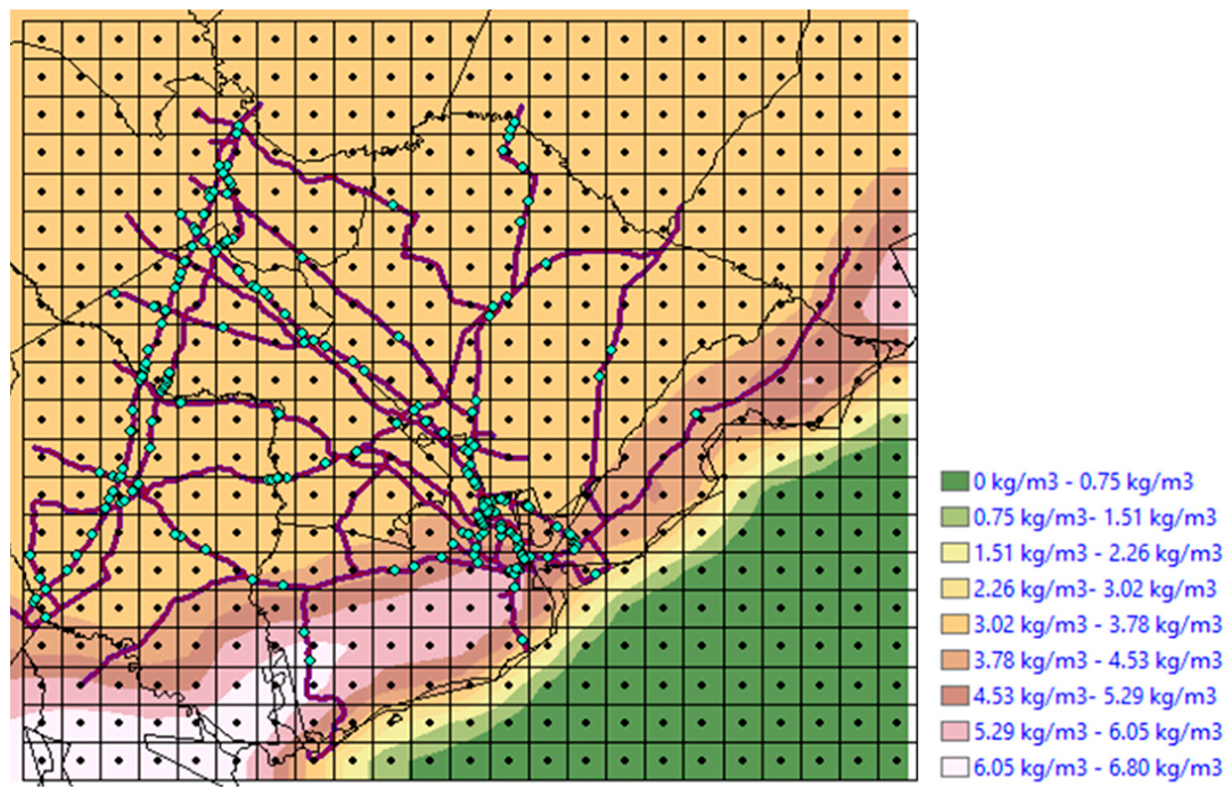
4. Benchmark Problem: A Highway Network in South Carolina, USA

4.1. Overview

In this section, the proposed seismic resilience assessment model is illustrated with a highway network in South Carolina (see Figure 5) which is similar to and was previously used as a case study by Rokneddin et al. [42]. This network is selected as a benchmark problem in this study because the surrogate seismic fragility curves of various types of bridges located in the network are available [35], which allows us not to develop the surrogate models on our own through extensive structural analyses. As indicated by Rokneddin et al. [42], the network consists of bridges that are vulnerable to earthquake activity due to a lack of seismic design and retrofit. The bridges in the network are also potentially exposed to marine chloride due to their proximity to the Atlantic Ocean, as shown in Figure 5, which makes these bridges more vulnerable to earthquakes over time.
For the purpose of illustration, a scenario-based approach is taken in this paper to quantify and reduce uncertainties along the process of seismic resilience assessment through information entropy and dynamic BN. It should be noted that uncertainties in earthquake hazard intensity, location, frequency, and timing can be quantified by following the same procedure that will be introduced for other random variables (chloride concentration and traffic demand) in the remaining section. Earthquake-related uncertainties are not considered in this benchmark problem because (a) these uncertainties are more like irreducible aleatory uncertainties and (b) probabilistic seismic hazard analysis may require additional computational burden. The scenario earthquake event considered is the 1886 Charleston earthquake, one of the most damaging earthquakes in the Eastern United States. Its estimated moment magnitude was 6.9–7.3 Mw, and over 2000 buildings were damaged.
Information about the bridges in the network is obtained from the national bridge inventory database. Based on the number of spans, major construction materials, and types of design/construction, the bridges are categorized into five different classes. The bridges are further classified based on their proximity to the ocean: marine splash zone for the bridges within 10 m from the coastline and marine atmospheric zone for the bridges outside the splash zone. Each category of bridges possesses unique surrogate seismic fragility curves to account for the influence of corrosion on the bridge’s ability to withstand seismic forces over time.

4.2. Dynamic Bayesian Updating with Field-Measurement Data

To examine the role of investigating and monitoring major random variables (specifically surface chloride concentration and traffic demand) in resilience assessment, this study considers three cases: (a) Case A: the baseline case where transportation resilience is measured based on the prior probability distributions of random variables, which is consistent with most existing studies introduced in the literature review; (b) Case B: true transportation resilience, which is never known in the real world; and (3) Case C: the case where transportation resilience is measured based on the updated posterior probability distributions of random variables. Figure 6 illustrates the dynamic BN embedded in the proposed seismic resilience assessment, which represents Case C. More specifically, in Case C, it is assumed that two random variables that change over time—surface chloride concentration and traffic demand—are monitored and that their prior probability distributions are updated over time through dynamic BN.
Input vector ( x ) and logistic regression coefficients ( θ ) of the parameterized fragility curve equation (i.e., Equation (6)) vary depending on the class of bridge and the provision of seismic detailing. Among them, the area of rebar is one of the key parameters and is included in the fragility curves of all bridge classes regardless of its seismic detailing. As described in Section 3.1, surface chloride corrosion may induce a reduction in the area of rebar and ultimately affects time-dependent failure probabilities of bridges, which affects both bridge and link capacities (Section 3.2). Therefore, monitoring data on surface chloride corrosion at all bridge locations over time may improve our understanding of time-dependent bridge and network capacity. On the other hand, traffic demand at each highway link also changes over time due to population changes [17], land-use conditions [43], infrastructure development, intelligent transport system [44], and policies related to traffic-control technologies (e.g., ramp metering, road pricing, route guidance, and variable speed limits) [45]. Thus, monitoring and updating traffic demand over time may improve the accuracy of network performance assessment. By combining these two time-dependent random variables for all the links in the network, network performance is assessed and updated at every time step.
For Case A, the prior probability distributions of surface chloride concentration for bridges vary depending on bridge location and construction year. Prior knowledge suggests that the surface chloride concentration is lognormally distributed with the mean values adopted from Ghosh [35] and a coefficient of variation of 0.5. While these prior distributions consider randomness in C s , they cannot capture the time-dependent characteristics of chloride concentration as many static resilience assessment studies do. Due to epistemic uncertainties, true time-dependent chloride concentrations on the surface (i.e., Case B) are never known in the real world. Thus, in this study, we generate synthetic true C s values by randomly sampling its initial value from the prior distributions and applying Equation (16) to generate time-dependent C s over a 50 year period [46].
C s , t ( t ) = C 0 + α ln t                                            
where C 0 = the surface chloride concentration at the beginning and α = the constant value of 0.6856. The procedure described above, however, does not account for spatial correlation in the surface chloride concentrations between adjacent locations, which has been identified as one of the factors that may affect the accuracy of time-dependent bridge functionality estimation. To generate spatially correlated chloride concentration values, the Kriging spatial interpolation technique is used. According to the exponential variogram for surface chloride concentration provided by Ghosh [35], the “range” is 8 km, where semivariance reaches a plateau and observations are no longer spatially correlated. Therefore, we first divide the entire case-study region into 8 km × 8 km cells and randomly generate the initial surface chloride concentration at the centroid of each cell. It is because the distance between two centroids is equal to the “range” and initial chloride concentrations at these centroids are not spatially correlated and can be randomly generated from the prior distributions. Then, the Kriging technique is used to calculate C s , t ( t ) at the locations between the centroids, as illustrated in Figure 7. In the next time step, Equation (16) is applied to generate surface chloride concentration only at the centroids and, then, the Kriging technique is used to generate spatially correlated values over the network. This procedure is repeated until the end of a 50 year time period. The time-dependent surface chloride concentration values are used to update the area of rebar at each bridge location (See Equations (3) and (4)), which are subsequently used as an input to the time-dependent fragility curve.
For Case C, the surface chloride concentration values are monitored over time and Bayesian updating is employed to update the probability distributions of C s and the time-dependent fragility curves. In this study, synthetic measurement data are generated. These plausible measurement-data realizations are generated by combining the true value with a random error term as follows:
C s , m t = C s , t t + ε e
where C s , m ( t ) = the time series measurement data; C s , t t = the true values or ideal data; and ε e = the measurement error reflecting our confidence in the measurement data. Given that the true data will never be known exactly, the measurement data can be used to better represent the true states of surface chloride concentrations. In this study, the PDFs of surface chloride concentration P C s ( C s , t ) at all bridge locations are updated based on the synthetic measurement data through dynamic BN. Subsequently, the posterior PDFs of P C s ( C s , t ) are used to update the time-dependent fragility functions.
Similarly, we generate synthetic values of traffic demand for the three cases. The annual average daily traffic (AADT) data obtained from the South Carolina Department of Transportation (SCDOT) are used to predict the theoretical traffic demands over the next 50 years. SCDOT provides AADT data that have been collected from sensors placed on the road network in the past 17 years. This study specifically uses an autoregressive integrated moving average (ARIMA) model in generating the theoretical values of traffic demands because ARIMA models can (a) capture the seasonality and long-term trends that the AADT data exhibit and (b) provide accurate forecasts for both short- and medium-term AADT predictions. In this study, the R software is used in fitting and forecasting the traffic demand. After generating the theoretical (simulated) values of traffic demand using the ARIMA model, the synthetic true values and synthetic measurement data are generated based on the following equations, respectively:
y t x = y a x , θ + ε a
y m x = y t x + ε o b s
where x = the set of independent variables; y t x = the synthetic true values of traffic demand; θ = the set of model parameters; y a x , θ = the outputs of the ARIMA model, that are the theoretical values of traffic demand; ε a = the modeling error; y m x = the synthetic measurement data on traffic demand; and ε o b s = the measurement error which is usually modeled as a Gaussian random variable. In general, the measurement error is smaller than the modeling error. To clarify, the theoretical values, y a x , θ , are used for traffic demand in Case A, the synthetic true values, y t x , are used in Case B, and the synthetic measurement data, y m x , are used in Case C.
The reliability of the data obtained from Inspection or monitoring programs Is crucial for an accurate performance and resilience assessment of transportation systems. Inaccurate data can lead to an incorrect assessment, which can have serious consequences for the safety and reliability of the transportation system. Therefore, in this study, a sensitivity analysis is performed to evaluate how data reliability affects the accuracy of the estimation of system performance and resilience. By doing so, it is possible to determine the level of confidence in the resilience assessment results and make informed decisions about maintenance and repair strategies. In this study, a range of equipment with different accuracies is considered. To simplify the modeling procedure, the coefficient of variation of the modeling error term ( ε o b s in Equation (19)) is chosen as the representative metric, which ranges from 0.05 to 0.3 in increments of 0.05. This range represents the variability in the accuracy of the equipment being used.

4.3. Network Analysis and Seismic Resilience Assessment

To perform a network analysis, we first determine the capacities and demands of all the links in the network. Conditioned on the 1886 Charleston earthquake, a ground motion intensity map in the study region is generated through Open-Source Seismic Hazard Analysis (OpenSHA) [47]. While a set of ground motion intensity maps should be generated for the scenario earthquake to account for uncertainties, only the median values of ground motion intensities are used in this paper for the purpose of simplification. Figure 8 shows the ground motion intensity map generated through OpenSHA. By combining the ground motion intensity at every bridge location with the corresponding seismic fragility curves, we can find the failure probabilities of all the bridges. This process is coupled with ArcGIS and data on bridges and highway segments. If any form of retrofit or rehabilitation has been implemented on a bridge prior to an earthquake event, the enhanced structural capacity resulting from these interventions can be incorporated into the fragility curve. It should be noted that these failure probabilities are updated over time because time-dependent fragility curves are updated based on the measurement data.
The updated probability of failure of each bridge, that is the result of the parameterized fragility function, is converted into the reliability index ( β ). Ghasemi and Lee [37] proposed a reliability-based indicator for assessing the expected post-earthquake traffic flow capacity of a highway bridge. The relationship between the reliability index and the post-earthquake traffic carrying capacity ( T C C ) is shown in the following equation [37]:
T C C = 0.2432 e 0.3548 β
This study assumes that bridges play a key role in determining transportation-network performance and that the bridges on the same link can be modeled as a series system. At every time step, the reliability indices of all bridges are updated based on the measurement data and are converted into their post-earthquake traffic-carrying capacities and the associated link capacities. The link capacities are used as inputs to the CUBE voyager software program to measure network performance. In addition, the updated traffic demands for all links are also incorporated into the network analysis so that both updated link capacity and link demand affect the performance of the network.
The network performance Is measured by the total travel time, T T T t . After the 50 year performance profile of the network is obtained, the time-dependent resilience of the case-study network is calculated using Equation (9). Finally, the information entropy of each node in the Bayesian network is calculated, and their sum gives the total information entropy of the system.

5. Results and Discussion

To estimate the bridges’ failure probabilities, the parameterized fragility curve equations are utilized in this study. Figure 9a shows the fragility curves of a specific bridge for different years under Case C. The fragility curves are updated over time due to the reassessed posterior PDFs of chloride concentration values obtained through dynamic BN. This figure shows how the probability of failure increases with time due to the effect of corrosion-induced deterioration.
Figure 9b compares the fragility curves of a bridge for Cases A, B, and C at Year 50. This comparison allows for an assessment of the accuracy of the theoretical (Case A) and updated (Case C) values compared to the true values (Case B). The results demonstrate the significance of monitoring and inspection programs in improving the accuracy of bridge fragility assessments. As expected, the updated fragility curve based on field-measurement data is much closer to the true fragility curve, which indicates that the proposed dynamic BN method can estimate bridge-failure probability in a more accurate manner compared to using only prior theoretical information. Given that the true fragility curve is never known in the real world, the proposed dynamic BN model offers a reliable and practical way to improve our knowledge about major deterioration-related random variables and, ultimately, enhance our prediction about bridge-failure probability. Similar observations can be found in the comparison of traffic demands between Cases A, B, and C.
To estimate the total travel time for the case-study network, while incorporating time-dependent link capacity and demands, CUBE simulates the movement of vehicles and traffic flow through the network over time by taking into account factors such as congestion, signal timing, and speed limits. The total travel time obtained from the CUBE simulation is incorporated into Equation (10) to evaluate the performance of the case-study network. Figure 10 shows a time-dependent seismic resilience index calculated from Equation (9) following the scenario earthquake event. Overall, the seismic resilience index decreases over time mainly due to bridge deterioration and increased traffic demands. Another finding is that as time increases, the degree of overestimation of network seismic resilience by Case A increases. Conversely, Case C maintains a consistent and accurate estimate of network seismic resilience, even in the distant future. This also highlights the significance of monitoring and inspection programs in reducing uncertainties. However, it should be noted that there is some deviation between Cases B and C, which can be attributed to measurement errors. Such errors may occur due to various factors such as equipment limitations, human error, etc. These errors can affect the accuracy of the data and consequently impact the estimation of total travel time, network performance, and seismic resilience.
To investigate how the reliability of monitoring and inspection equipment can impact the accuracy of the seismic resilience assessment results for the case-study network over time, a sensitivity analysis is performed. A range of equipment with different levels of reliability is included in the sensitivity analysis, with a coefficient of variation (CoV) values of the measurement-error term ranging from 0.05 to 0.3. More specifically, the CoV of ε e in Equation (17) and the CoV of ε o b s in Equation (19) vary for chloride concentration and traffic demand, respectively. In the case where the CoV is 0, Case C becomes identical to the true case (i.e., Case B). Figure 11 shows the sensitivity analysis results of network seismic resilience to the reliability of monitoring equipment. The figure compares the 95% confidence intervals of the seismic resilience index for the equipment with the highest reliability (i.e., CoV of 0.05) and the lowest reliability (i.e., CoV of 0.3). The outcomes of Case B lie between the 95% confidence intervals of both types of equipment, with the exception of the 30 year mark. As this deviation is primarily due to the limited number of simulations, it is expected that the outcomes of B consistently fall within the confidence intervals of both cases with a larger number of simulations. As expected, the equipment with higher reliability is more accurate in predicting the true seismic resilience index. Thus, by utilizing high-reliability monitoring equipment, transportation managers can obtain more accurate and reliable resilience assessment results, make better informed decisions, and take effective necessary actions to improve the overall seismic resilience of the transportation network. The sensitivity analysis results can further be used to determine the level of monitoring equipment reliability that is required to achieve the desired level of accuracy in the seismic resilience assessment.
To quantify uncertainties along the process of the seismic resilience assessment, information entropy values for the two types of monitoring equipment with different levels of reliability (i.e., CoV of 0.05 and CoV of 0.3) are calculated using Equation (15). The results are then used to create Figure 12 and Figure 13. Figure 12a,b depict geographic maps of information entropy for bridge-failure probability at Year 50 when using higher reliability equipment (CoV of 0.05) and lower reliability equipment (CoV of 0.3), respectively. Each bridge has a unique information entropy value, which reflects different amounts of randomness or uncertainty. It is found that when lower reliability equipment is used, the information entropy values for the bridge-failure probability are higher, indicating a greater degree of uncertainty. Similar observations can be found in Figure 13, which compares information entropy values for traffic demand at Year 50 when it is monitored through higher reliability equipment (CoV of 0.05) and lower reliability equipment (CoV of 0.3).
Finally, the information entropy of the seismic resilience index is calculated. Due to the higher values of information entropy for the bridge-failure probability and traffic demand, the information entropy for the seismic resilience index is 21% higher at Year 50 when lower reliability equipment is used, compared to higher reliability equipment.
Figure 14 presents a percentage increase in information entropy with respect to the baseline value (i.e., Year 10 value) over time. This increase in information entropy over time for both cases suggests an increase in the amount of uncertainty in the process. This is an important finding because it highlights the need to carefully consider the reliability of the monitoring equipment used in the seismic resilience assessment to ensure accurate results. Additionally, the slower increase in information entropy over time when using higher reliability equipment indicates that epistemic uncertainty decreases more quickly over time, making it an attractive option for a long-term seismic resilience assessment. The practical applications of these findings include informing decisions about the selection of monitoring equipment for the seismic resilience assessment, as well as providing a framework for assessing uncertainties in the process. This information can be used to identify areas that require further investigation or intervention to improve the resilience of the transportation network in earthquake-prone regions.

6. Summary and Conclusions

This paper presented a dynamic BN-based resilience assessment model for a large-scale transportation network that can explicitly quantify uncertainties in all phases of the assessment and investigate the role of inspection and monitoring programs in uncertainty reduction. First, uncertainties in the transportation-network capacity and demand were identified and reduced through a dynamic BN based on measurement data collected over time. Subsequently, the updated link capacity and demand were incorporated into the network analysis to update the seismic resilience index over time. The proposed model was then tested on a benchmark problem, a highway network in South Carolina, to demonstrate how the model could systematically quantify and reduce uncertainties when assessing the seismic resilience of the network. To further examine the significance of the measurement data in improving the accuracy of the prediction of the seismic resilience index, a sensitivity analysis was performed using different sets of data with varying reliabilities.
The benchmark problem results showed that incorporating monitoring and inspection data on important variables such as chloride concentration and traffic demands could improve predicting the seismic resilience of the network. It also suggested the need to consider equipment reliability when designing monitoring and inspection programs. These findings can assist transportation managers and policymakers in identifying necessary equipment reliability levels and prioritizing inspection and monitoring efforts. The impact of this paper is significant as it provides decisionmakers with the tools to better manage transportation-system resilience in the face of natural hazards and uncertainty. The results can be used to determine which monitoring/inspection techniques to prioritize, evaluate the effectiveness of current techniques, and perform cost–benefit analyses for optimal resource allocation.

Author Contributions

Conceptualization, J.Y.L.; methodology, J.Y.L., V.J. and S.H.G.; simulation: V.J. and J.Z.; writing—original draft preparation, V.J. and J.Y.L.; writing—review and editing, J.Z. and S.H.G.; visualization: V.J.; supervision, J.Y.L.; funding acquisition: J.Y.L. All authors have read and agreed to the published version of the manuscript.

Funding

This work was sponsored by the National Center for Transportation Infrastructure Durability and Life Extension (TriDurLE). This support is gratefully acknowledged. Any opinions, findings, conclusions, or recommendations expressed in this material are those of the authors and do not necessarily reflect the views of TriDurLE.

Data Availability Statement

The data that support the findings of this study are available from the corresponding author upon reasonable request.

Conflicts of Interest

The authors declare no conflict of interest. The funders had no role in the design of the study; in the collection, analyses, or interpretation of data; in the writing of the manuscript; or in the decision to publish the results.

References

  1. Zhou, Y.; Wang, J.; Yang, H. Resilience of transportation systems: Concepts and comprehensive review. IEEE Trans. Intell. Transp. Syst. 2019, 20, 4262–4276. [Google Scholar] [CrossRef]
  2. Bruneau, M.; Chang, S.E.; Eguchi, R.T.; Lee, G.C.; O’Rourke, T.D.; Reinhorn, A.M.; Shinozuka, M.; Tierney, K.; Wallace, W.A.; Von Winterfeldt, D. A framework to quantitatively assess and enhance the seismic resilience of communities. Earthq. Spectra 2003, 19, 733–752. [Google Scholar] [CrossRef]
  3. Chang, S.E.; Shinozuka, M. Measuring improvements in the disaster resilience of communities. Earthq. Spectra 2004, 20, 739–755. [Google Scholar] [CrossRef]
  4. Bruneau, M.; Reinhorn, A. Overview of the resilience concept. In Proceedings of the 8th U.S. National Conference on Earthquake Engineering, San Francisco, CA, USA, 18–22 April 2006; Volume 2040, pp. 18–22. [Google Scholar]
  5. Madni, A.M.; Jackson, S. Towards a conceptual framework for resilience engineering. IEEE Syst. J. 2009, 3, 181–191. [Google Scholar] [CrossRef]
  6. Meerow, S.; Newell, J.P.; Stults, M. Defining urban resilience: A review. Landsc. Urban Plan. 2016, 147, 38–49. [Google Scholar] [CrossRef]
  7. Bostick, T.P.; Connelly, E.B.; Lambert, J.H.; Linkov, I. Resilience science, policy and investment for civil infrastructure. Reliab. Eng. Syst. Saf. 2018, 175, 19–23. [Google Scholar] [CrossRef]
  8. Berche, B.; Von Ferber, C.; Holovatch, T.; Holovatch, Y. Resilience of public transport networks against attacks. Eur. Phys. J. B 2009, 71, 125–137. [Google Scholar] [CrossRef]
  9. Murray-Tuite, P.M. A comparison of transportation network resilience under simulated system optimum and user equilibrium conditions. In Proceedings of the 2006 Winter Simulation Conference, Monterey, CA, USA, 3–6 December 2006; IEEE: New York, NY, USA, 2006; pp. 1398–1405. [Google Scholar]
  10. Adams, T.M.; Bekkem, K.R.; Toledo-Durán, E.J. Freight resilience measures. J. Transp. Eng. 2012, 138, 1403–1409. [Google Scholar] [CrossRef]
  11. Ip, W.H.; Wang, D. Resilience evaluation approach of transportation networks. In Proceedings of the 2009 International Joint Conference on Computational Sciences and Optimization, Sanya, China, 24–26 April 2009; IEEE: New York, NY, USA, 2009; Volume 2, pp. 618–622. [Google Scholar]
  12. Cox, A.; Prager, F.; Rose, A. Transportation security and the role of resilience: A foundation for operational metrics. Transp. Policy 2011, 18, 307–317. [Google Scholar] [CrossRef]
  13. Liao, T.Y.; Hu, T.Y.; Ko, Y.N. A resilience optimization model for transportation networks under disasters. Nat. Hazards 2018, 93, 469–489. [Google Scholar] [CrossRef]
  14. Zhang, X.; Miller-Hooks, E.; Denny, K. Assessing the role of network topology in transportation network resilience. J. Transp. Geogr. 2015, 46, 35–45. [Google Scholar] [CrossRef]
  15. Ganin, A.A.; Kitsak, M.; Marchese, D.; Keisler, J.M.; Seager, T.; Linkov, I. Resilience and efficiency in transportation networks. Sci. Adv. 2017, 3, e1701079. [Google Scholar] [CrossRef]
  16. Ouyang, M.; Dueñas-Osorio, L.; Min, X. A three-stage resilience analysis framework for urban infrastructure systems. Struct. Saf. 2012, 36, 23–31. [Google Scholar] [CrossRef]
  17. Zhao, J.; Lee, J.Y.; Wolcott, M.P. Multi-component resilience assessment framework for transportation systems. In Proceedings of the 13th International Conference on Structural Safety and Reliability 2022, Shanghai, China, 20–24 June 2021. [Google Scholar]
  18. Dui, H.; Liu, K.; Wu, S. Data-driven reliability and resilience measure of transportation systems considering disaster levels. Ann. Oper. Res. 2023. [Google Scholar] [CrossRef]
  19. Yang, Y.; Pan, S.; Ballot, E. Freight transportation resilience enabled by physical internet. IFAC-Pap. 2017, 50, 2278–2283. [Google Scholar] [CrossRef]
  20. Otuoze, S.H.; Hunt, D.V.; Jefferson, I. Neural network approach to modelling transport system resilience for major cities: Case studies of lagos and kano (Nigeria). Sustainability 2021, 13, 1371. [Google Scholar] [CrossRef]
  21. Wang, H.W.; Peng, Z.R.; Wang, D.; Meng, Y.; Wu, T.; Sun, W.; Lu, Q.C. Evaluation and prediction of transportation resilience under extreme weather events: A diffusion graph convolutional approach. Transp. Res. Part C Emerg. Technol. 2020, 115, 102619. [Google Scholar] [CrossRef]
  22. John, A.; Yang, Z.; Riahi, R.; Wang, J. A risk assessment approach to improve the resilience of a seaport system using Bayesian networks. Ocean. Eng. 2016, 111, 136–147. [Google Scholar] [CrossRef]
  23. Hosseini, S.; Barker, K. Modeling infrastructure resilience using Bayesian networks: A case study of inland waterway ports. Comput. Ind. Eng. 2016, 93, 252–266. [Google Scholar] [CrossRef]
  24. Castillo, E.; Grande, Z.; Calviño, A. Bayesian networks-based probabilistic safety analysis for railway lines. Comput.-Aided Civ. Infrastruct. Eng. 2016, 31, 681–700. [Google Scholar] [CrossRef]
  25. Kammouh, O.; Gardoni, P.; Cimellaro, G.P. Probabilistic framework to evaluate the resilience of engineering systems using Bayesian and dynamic Bayesian networks. Reliab. Eng. Syst. Saf. 2020, 198, 106813. [Google Scholar] [CrossRef]
  26. Frangopol, D.M.; Nakib, R. Redundancy in highway bridges. Eng. J. 1991, 2003, 28. [Google Scholar]
  27. Mackie, K.R.; Stojadinović, B. Post-earthquake functionality of highway overpass bridges. Earthq. Eng. Struct. Dyn. 2006, 35, 77–93. [Google Scholar] [CrossRef]
  28. Padgett, J.E.; DesRoches, R. Bridge functionality relationships for improved seismic risk assessment of transportation networks. Earthq. Spectra 2007, 23, 115–130. [Google Scholar] [CrossRef]
  29. Shiraki, N.; Shinozuka, M.; Moore, J.E.; Chang, S.E.; Kameda, H.; Tanaka, S. System risk curves: Probabilistic performance scenarios for highway networks subject to earthquake damage. J. Infrastruct. Syst. 2007, 13, 43–54. [Google Scholar] [CrossRef]
  30. Atadero, R.A.; Jia, G.; Abdallah, A.; Ozbek, M.E. An integrated uncertainty-based bridge inspection decision framework with application to concrete bridge decks. Infrastructures 2019, 4, 50. [Google Scholar] [CrossRef]
  31. Bu, L.; Qiao, L.; Sun, R.; Lu, W.; Guan, Y.; Gao, N.; Hu, X.; Li, Z.; Wang, L.; Tian, Y.; et al. Time and crack width dependent model of chloride transportation in engineered cementitious composites (ECC). Materials 2022, 15, 5611. [Google Scholar] [CrossRef] [PubMed]
  32. Gong, C.; Frangopol, D.M. Condition-Based Multiobjective Maintenance Decision Making for Highway Bridges Considering Risk Perceptions. J. Struct. Eng. 2020, 146, 04020051. [Google Scholar] [CrossRef]
  33. Thoft-Christensen, P.; Jensen, F.M.; Middleton, C.R.; Blackmore, A. Assessment of the Reliability of Concrete Slab Bridges; Structural Reliability Theory; Dept. of Building Technology and Structural Engineering: Aalborg, Denmark, 1996; Volume R9616, No. 157. [Google Scholar]
  34. Stewart, M.G.; Rosowsky, D.V. Time-dependent reliability of deteriorating reinforced concrete bridge decks. Struct. Saf. 1998, 20, 91–109. [Google Scholar] [CrossRef]
  35. Ghosh, J. Parameterized Seismic Reliability Assessment and Life-Cycle Analysis of Aging Highway Bridges. Doctoral Dissertation, Rice University, Houston, TX, USA, 2013. [Google Scholar]
  36. Ghosh, J.; Rokneddin, K.; Padgett, J.E.; Dueñas-Osorio, L. Seismic reliability assessment of aging highway bridge networks with field instrumentation data and correlated failures, I: Methodology. Earthq. Spectra 2014, 30, 795–817. [Google Scholar] [CrossRef]
  37. Ghasemi, S.H.; Lee, J.Y. Reliability-based indicator for post-earthquake traffic flow capacity of a highway bridge. Struct. Saf. 2021, 89, 102039. [Google Scholar] [CrossRef]
  38. Chen, A.; Kasikitwiwat, P.; Yang, C. Alternate capacity reliability measures for transportation networks. J. Adv. Transp. 2013, 47, 79–104. [Google Scholar] [CrossRef]
  39. Kezhiyur, A.J. Analysis of Age-Dependent Resilience for a Highway Network with Aging Bridges. Master’s Thesis, Pennsylvania State University, State College, PA, USA, 2015. [Google Scholar]
  40. Shannon, C. Claude Shannon. Inf. Theory 1948, 3, 224. [Google Scholar]
  41. Parhizkar, T.; Balali, S.; Mosleh, A. An entropy based bayesian network framework for system health monitoring. Entropy 2018, 20, 416. [Google Scholar] [CrossRef] [PubMed]
  42. Rokneddin, K.; Ghosh, J.; Dueñas-Osorio, L.; Padgett, J.E. Seismic reliability assessment of aging highway bridge networks with field instrumentation data and correlated failures, II: Application. Earthq. Spectra 2014, 30, 819–843. [Google Scholar] [CrossRef]
  43. Faghih-Imani, A.; Eluru, N.; El-Geneidy, A.M.; Rabbat, M.; Haq, U. How land-use and urban form impact bicycle flows: Evidence from the bicycle-sharing system (BIXI) in Montreal. J. Transp. Geogr. 2014, 41, 306–314. [Google Scholar] [CrossRef]
  44. Kaparias, I.; Eden, N.; Tsakarestos, A.; Gal-Tzur, A.; Gerstenberger, M.; Hoadley, S.; Lefebvre, P.; Ledoux, J.; Bell, M. Development and application of an evaluation framework for urban traffic management and Intelligent Transport Systems. Procedia-Soc. Behav. Sci. 2012, 48, 3102–3112. [Google Scholar] [CrossRef]
  45. Marchau, V.A.; Walker, W.E.; Van Wee, G.P. Dynamic adaptive transport policies for handling deep uncertainty. Technol. Forecast. Soc. Chang. 2010, 77, 940–950. [Google Scholar] [CrossRef]
  46. Song, H.W.; Lee, C.H.; Ann, K.Y. Factors influencing chloride transport in concrete structures exposed to marine environments. Cem. Concr. Compos. 2008, 30, 113–121. [Google Scholar] [CrossRef]
  47. Field, E.H.; Jordan, T.H.; Cornell, C.A. OpenSHA: A Developing community-modeling environment for seismic hazard analysis. Seism. Res. Lett. 2003, 74, 406–419. [Google Scholar] [CrossRef]
Figure 1. Overall flowchart showing a procedure for the proposed model.
Infrastructures 08 00128 g001
Figure 2. Time-dependent performance profile of a bridge subjected to the combined effect of earthquake and corrosion.
Infrastructures 08 00128 g002
Figure 3. A conceptual representation of the time-dependent performance of a structure (adopted from Bruneau et al. [2]).
Infrastructures 08 00128 g003
Figure 4. Conceptual representation of a series of probabilistic dependencies in the proposed resilience assessment model.
Infrastructures 08 00128 g004
Figure 5. The geographic distribution of the highway network.
Infrastructures 08 00128 g005
Figure 6. Dynamic Bayesian network embedded in seismic resilience assessment.
Infrastructures 08 00128 g006
Figure 7. Result from spatial Kriging of surface chloride concentration at Year 50.
Infrastructures 08 00128 g007
Figure 8. Ground motion intensity map for the study region.
Infrastructures 08 00128 g008
Figure 9. (a) Fragility curves of a specific bridge for different years (Case C); (b) Comparison between Cases A, B, and C: fragility curves of a bridge at Year 50.
Infrastructures 08 00128 g009
Figure 10. Time-dependent resilience index of the network following the scenario earthquake event: comparison of three cases.
Infrastructures 08 00128 g010
Figure 11. Sensitivity analysis results of network seismic resilience index to the reliability of monitoring equipment (95% confidence interval).
Infrastructures 08 00128 g011
Figure 12. Geographic distribution of information entropy for bridge-failure probability at Year 50: (a) using higher reliability equipment; (b) using lower reliability equipment.
Infrastructures 08 00128 g012
Figure 13. Geographic distribution of information entropy for traffic demand at Year 50: (a) using higher reliability equipment; (b) using lower reliability equipment.
Infrastructures 08 00128 g013
Figure 14. Percentage increase in information entropy with respect to the baseline value (i.e., Year 10 value) over time: higher and lower reliability monitoring equipment.
Infrastructures 08 00128 g014
Disclaimer/Publisher’s Note: The statements, opinions and data contained in all publications are solely those of the individual author(s) and contributor(s) and not of MDPI and/or the editor(s). MDPI and/or the editor(s) disclaim responsibility for any injury to people or property resulting from any ideas, methods, instructions or products referred to in the content.

