Minimum-Lap-Time Planning of Multibody Vehicle Models via the Articulated-Body Algorithm

Abstract

Minimum lap-time planning (MLTP) is a well-established problem in the race car industry to provide guidelines for drivers and optimize the vehicle’s setup. In this paper, we tackle the 3D nature of the problem in its full extension, making no simplifying assumptions on the mechanics of the system. We propose a multibody vehicle model, described by rigorous dynamical equations. To effectively handle the resulting complexity, we devised an efficient direct dynamics computational method based on Featherstone’s articulated-body algorithm (ABA). To solve the MLTP, we employed a direct-collocation technique, discretizing the problem so that all information of the 3D track is pre-processed and directly embedded into the discrete problem. This discretization approach turns out to be perfectly compatible with our vehicle model, leading to a solution in accessible computational time frames. The high level of detail of the model makes the proposed approach most useful for in-depth vehicle dynamics analyses on complex tracks. To substantiate the analysis, we provide a comparison with the results obtained by a double-track model on the Nürburgring Nordschleife circuit. Consistently with the average trend defined by the double track, the proposed model features a more dynamically rich behavior, realistically capturing the higher-order effects elicited by the sharp corners and the highly variable slope of the track.

1. Introduction

Minimum lap-time planning problems (MLTPs) are well established in the race car industry, both to synthesize fast trajectories and to calibrate setup parameters optimally. In the technical literature, different methods have been proposed to solve MLTPs. A rich overview on their development is given in [1].

In general, two are the main approaches to tackle MLTPs. These are the quasi-steady-state technique and the method relying on the solution of an optimal control problem (OCP). Methods in the first class start from a predetermined path on the racetrack and build an acceleration profile on top of it. On the other hand, the second class is grounded on OC theory and defines all state trajectories as the solution of a purposely designed optimal control problem. Everything is discovered from scratch: the vehicle motion, the racing line and the controls that generate them.

Optimal control problems, in turn, can be solved either via an indirect method or a direct one. Both have been employed to solve MLTPs such as the one we will consider. A detailed description of these approaches can be found in [2], while an assessment of their pros and cons can be found in [3]. The indirect approach uses Pontryagin’s minimum principle to derive first-order optimality conditions. These lead to a two-point boundary value problem that has to be integrated. We find this approach employed for MLTP in [4,5]. The direct approach, on the other hand, aims to recast (transcript) the original OCP into a nonlinear program (NLP), to be solved numerically. In [6,7,8], this approach is employed to solve MLTPs. In most cases, as in the case of the present contribution, direct collocation is used as the transcription method.

To effectively formulate the OCP, the dynamical equations of the system must be at hand. They must be explicitly known and directly manipulable. Many of the works mentioned above rely on simple single-track or double-track vehicle models, as they appear in vehicle dynamics textbooks [1,9,10]. When a multibody approach is employed, e.g., in [4,7,11], the final equations are almost always simplified and greatly approximated.

In this paper, we propose a comprehensive and systematic multibody approach. The basic structure of our model is built around Featherstone’s articulated-body algorithm (ABA) [12]. The ABA is a powerful direct dynamics computational method, appearing in many different variants within the robotics literature [13,14,15]. To model the other, more specialized components of the system (such as tires and aerodynamics), we relied on conventional vehicle dynamics results [9,16,17,18].

The proposed approach opens up the possibility of thorough vehicle dynamics analysis similar to that offered by conventional simulation softwares such as CarSim or MBS Adams, which, on the downside, give limited access to their equations and cannot be easily embedded into the loop of an MLTP optimization problem.

As far as the track model is concerned, in most of the aforementioned works the track is either planar or is immersed into the system dynamics through Frenet–Serret equations involving torsion and curvature [5]. In the present work, as in [8,19], we embed the track features directly into the fixed structure of our nonlinear program, so that a fully 3D track can be considered, and all issues related to the Frenet–Serret formulation are avoided.

2. Vehicle Model

This section presents the topology of our multibody vehicle model and provides a characterization of its components. In Section 2.1 we introduce the bodies composing the model and explain their interconnection. Then, we focus on the modeling of suspension systems in Section 2.2 and we describe the tire model in Section 2.3. Finally, in Section 2.4, we detail the contributions of the external forces acting on the vehicle.

2.1. Topology of the Kinematic Tree and Its Parametrization

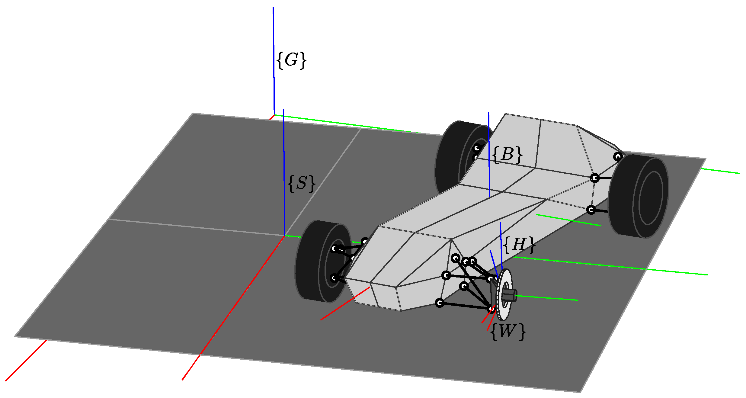
We model the vehicle as an articulated system of rigid bodies. In particular, our model includes the chassis, knuckles and wheels. The chassis represents the ensemble of all sprung masses of the vehicle, including the vehicle’s bearing framework, the motor, the driver and any other load carried onboard the car. These parts are assumed to have a fixed position with respect to one another. The wheels are the ensemble of the hubs, rims, tires and all other parts that rotate with them. In order to decouple the rotational motion of the wheel (about its axle) from its vertical motion (due to suspension travel), we also need to introduce the hub carriers, or knuckles. All unsprung masses that do not actually rotate, such as the brake calipers, are considered as part of the knuckle body; we will assume these components to have negligible mass.

To keep track of the relative pose between bodies, we conveniently attach a reference frame to each of them. We define front-left-up (FLU) barycentral reference frames $\left\{B\right\}$, $\left\{H\right\}$, and $\left\{W\right\}$ to be attached to the chassis, to the knuckle, and the rim of the generic wheel, respectively, as illustrated in Figure 1. (We will often make use of the generic symbols $\left\{H\right\}$ and $\left\{W\right\}$ to denote the frames attached to the knuckle and rim of the particular wheel under consideration. If the need arises to make a distinction between different wheels, we will explicitly write $\left\{H_k\right\}$ and $\left\{W_k\right\}$, where $k=1,2,3,4$ when referring to the front-left (FL), front-right (FR), rear-left (RL) or rear-right (RR) wheel, respectively).

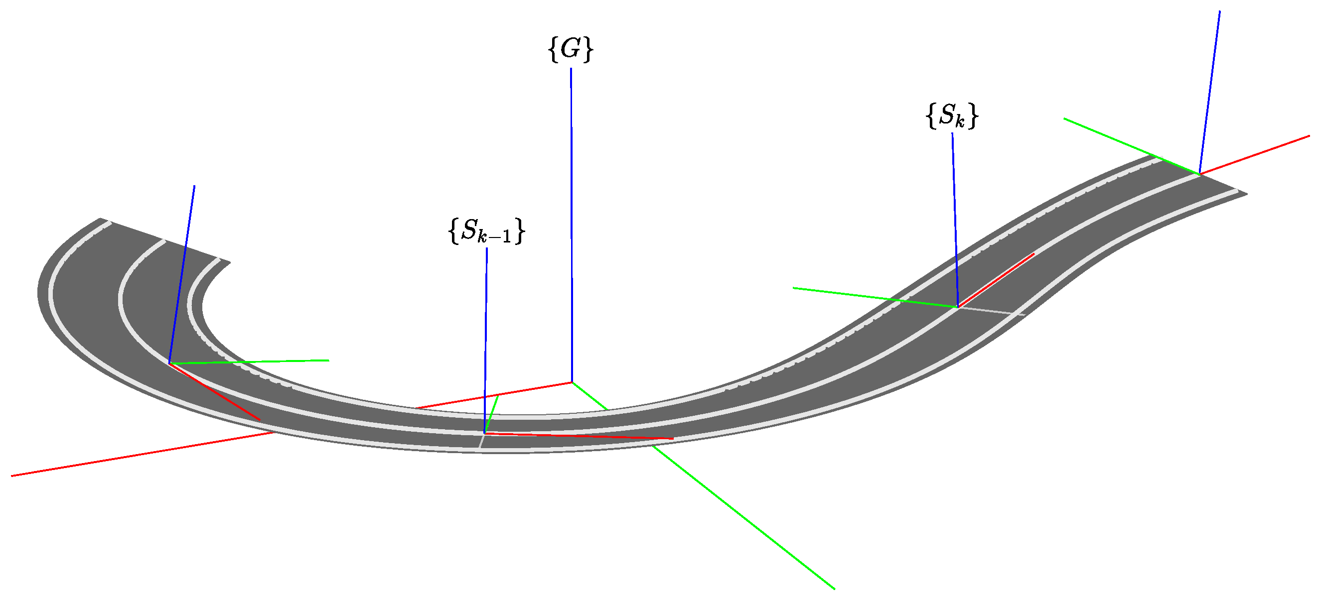
We also define an inertial reference frame $\left\{G\right\}$, fixed to ground, and an auxiliary frame $\left\{S\right\}$, following the vehicle on the track. More precisely, the track surface is modeled as a 3D ribbon [2] and the position of the vehicle on it is individuated by a point on its centerline curve. We set the origin $O_s$ of $\left\{S\right\}$ to coincide with this point, and the axis $x_s$ to be tangent to the centerline curve, pointing forward. The axis $y_s$ lies on the ribbon, pointing left, so that the axis $z_s$ points in the upward normal direction. As the vehicle travels along the track, the position of $\left\{S\right\}$ moves along the track centerline, and its orientation changes accordingly. At any moment, we assume that the vehicle is interacting with the $xy$-plane of $\left\{S\right\}$, tangent to the road surface.

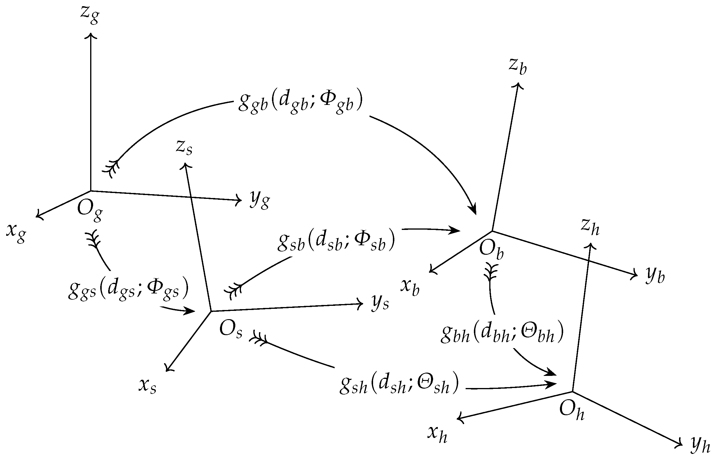
The relative position and orientation between each pair of frames are, respectively, described by three Cartesian coordinates $d\in {\mathbb{R}}^3$ and a rotation matrix $R\in SO\left(3\right)$, which we parameterize with three Euler angles $\Phi \in {\mathbb{R}}^3$. To describe the relative pose between frames, we use a homogeneous transformation matrix $g(d;\Phi )\in SE\left(3\right)$. To keep the equations more compact, we often gather the six coordinates d and $\Phi$ into a single configuration vector $q=(d;\Phi )$. A synoptic overview of the main transformations and their coordinates is provided in Figure 2.

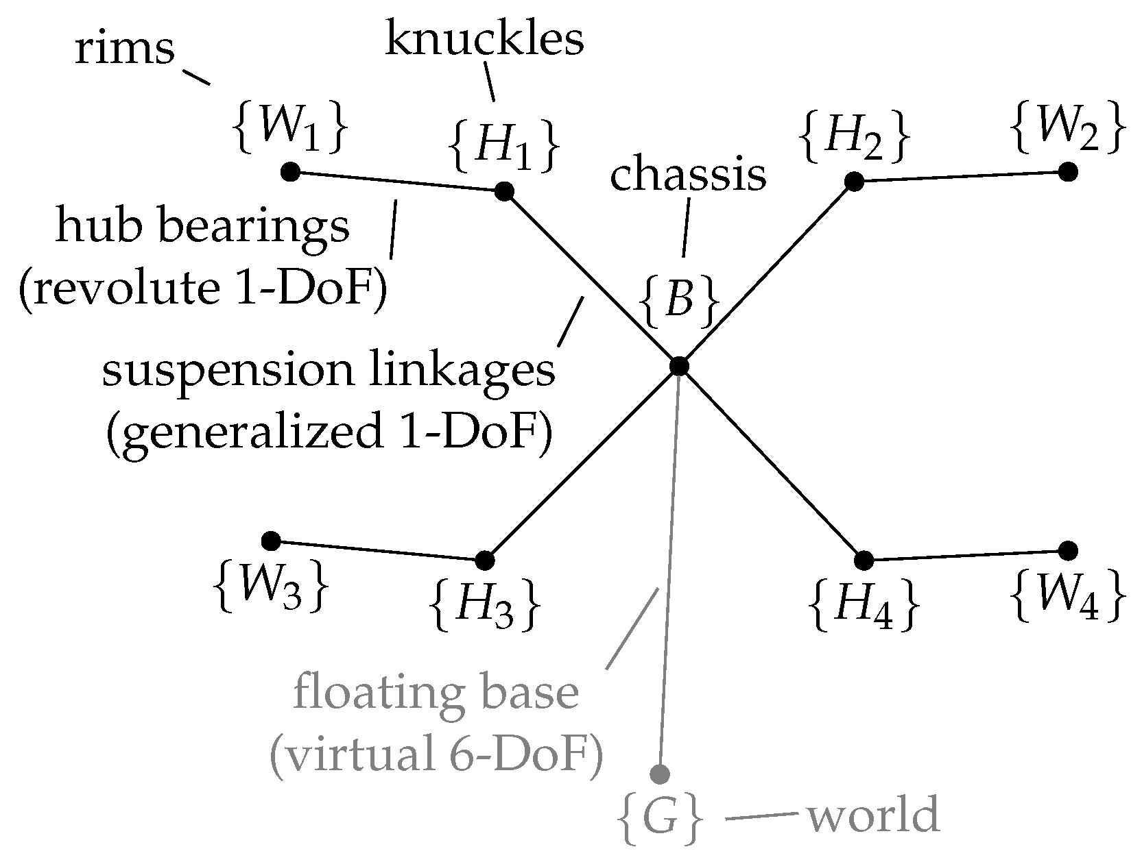
Within the articulated system, bodies are connected together by joints. As schematized by the graph in Figure 3, joints in our model are the hub bearings, connecting the rims $\left\{W\right\}$ to the knuckles $\left\{H\right\}$, and the suspension linkages, connecting the knuckles $\left\{H\right\}$ to the chassis $\left\{B\right\}$. The relative motion allowed by each of these joints enjoys one DoF. On the other hand, we observe that the chassis is a free-floating body and its pose with respect to ground is not constrained in any way. This behavior is encoded by a connection with the ground through a virtual six-DoF joint. Therefore, overall, the configuration of the vehicle enjoys a number of $4+4+6=14$ DoF.

Having defined the topology of our articulated system, we need to define a suitable set of variables to keep track of its configuration and motion. To this end, we associate every available degree of freedom with a position variable and a velocity variable.

To represent the configuration of the virtual six-DoF joint, we simply use the six coordinates $q_{gb}=(d_{gb};{\Phi }_{gb})$, as defined above. To represent its instantaneous motion, we conveniently adopt the driver’s point of view and we use the components of the linear velocity $v_{gb}$ of the origin of $\left\{B\right\}$ with respect to (w.r.t.) $\left\{G\right\}$ and of the angular velocity ${\omega }_{gb}$ of $\left\{B\right\}$ w.r.t. $\left\{G\right\}$, both expressed in the chassis frame $\left\{B\right\}$ components. We collect these components into a single vector $V_{gb}=(v_{gb};{\omega }_{gb})$, which we call the distal rigid-body velocity of $\left\{B\right\}$ w.r.t. $\left\{G\right\}$ expressed in $\left\{B\right\}$. The adjective distal reflects that these are expressed in the moving frame $\left\{B\right\}$ (as opposed to $\left\{G\right\}$, which would define proximal components). (In general, the rigid-body velocity of the form $V_{ij}^k$ would represent the instantaneous motion of frame $\left\{J\right\}$ w.r.t. frame $\left\{I\right\}$ expressed in components of the (observer) frame $\left\{K\right\}$. The generic $V_{ij}^k$ with $k\ne i,j$ are defined hybrid components. We recover the distal and the proximal components whenever $k=j$ and $k=i$, respectively. For notational brevity, we also make the following positions: $V_{gb}^b=V_{gb}=V_b$, $V_{gh}^h=V_{gh}=V_h$, $V_{gw}^h=V_w$, $V_{hw}^h=V_{hw}$, and $V_{bh}^h=V_{bh}$. Here, the central role as observers of frames $\left\{B\right\}$ and $\left\{H\right\}$ is apparent.)

To each of the four DoF allowed by the suspension system we associate a corresponding configuration variable z and its time derivative $\dot{z}$. Variable z is the suspension travel, the knowledge of which allows for the determination of the value of the six coordinates $q_{bh}=(d_{bh};{\Theta }_{bh})$. Similarly, given $\dot{z}$ (and z), one should be able to find the (distal) rigid-body velocity $V_{bh}=(v_{bh};{\omega }_{bh})$. Since the characterization of the suspension configuration in terms of a single variable is not trivial, its details are deferred to the next section. As far as the hub bearings are concerned, due to the assumed symmetrical properties of the wheel with respect to its axis, the (wheel) joint angle defining the orientation of $\left\{W\right\}$ w.r.t. $\left\{H\right\}$ is of no relevance for our analysis; what matters is only the joint velocity $\omega$, which is reasonably defined as the wheel speed.

2.2. Suspension Analysis

In this section we characterize the suspension system. The suspension connects the knuckles $\left\{H\right\}$ to the chassis $\left\{B\right\}$. The relative pose between $\left\{H\right\}$ and $\left\{B\right\}$ is encoded by the homogeneous transformation matrix $g_{bh}$, and parameterized by the six coordinates $q_{bh}$. To express $g_{bh}$ in terms of $q_{bh}$, we use the global product of exponentials (PoE) formula ([20], Section 3.2.2).

$$g_{bh}=e^{{\widehat{Y}}_1{q}_{bh,1}}\cdots e^{{\widehat{Y}}_6{q}_{bh,6}}{g}_{bh}\left(0\right),$$

(1)

where, in our case, the offset $g_{bh\left(0\right)}=I$ and $Y_1={[1,0,0,0,0,0]}^T$, $Y_2={[0,1,0,0,0,0]}^T$, $Y_3={[0,0,1,0,0,0]}^T$, $Y_4={[0,0,0,0,0,1]}^T$, $Y_5={[0,0,0,1,0,0]}^T$ and $Y_6={[0,0,0,0,1,0]}^T$ are the six normalized screw vectors associated with the Cartesian coordinates and Euler ZXY angles in $q_{bh}$. In this case, our exponentials are elementary transformation matrices, and the corresponding screw vectors have a very simple form. They can be interpreted as a parametrization of a virtual kinematic chain of three prismatic and three revolute joints connecting $\left\{H\right\}$ to $\left\{B\right\}$.

Obviously, the components of $q_{bh}$ are not independent variables. Rather, they are constrained by the particular suspension geometry and they are functions of the suspension travel z defined in Section 2.1, which can be chosen as the independent coordinate. Hereafter, we show how $q_{bh}$ is related to z. Along with z, the steering wheel angle $\delta$ may appear as an additional independent variable. (This is the general case of a wheel that can steer. For a front-steering vehicle, the dependence of $\delta$ is not present at the rear wheels, and the relative contributions can be omitted.) In general, the kinematic constraints can be expressed implicitly as a set of six scalar equations $F(q_{bh};z,\delta )=0\in {\mathbb{R}}^6$ in the six dependent variables $q_{bh}\in {\mathbb{R}}^6$ and the two independent variables $(z,\delta )\in {\mathbb{R}}^2$. The expression of the constraint function F depends on the particular suspension geometry of the vehicle under consideration; in Figure 1 a double-wishbone suspension is featured, but the analysis of any design is possible with the same approach. It is worth noting that, besides the five implicit equations associated to the double-wishbone constraints, an additional constraint must be included since no connection is initially assumed between $q_{bh}$ and $(z,\delta )$. In this development, we choose to define the suspension travel as the vertical displacement of the wheel center, and we used $z=d_{bh,3}$.

Under the hypotheses of the implicit function theorem [21], to establish an explicit functional relationship between $q_{bh}$ and $z,\delta$, we proceed as follows. First, we sample pairs $(z^{\left(p\right)},{\delta }^{\left(l\right)})$, with $p=1,\dots ,N$ and $l=1,\dots ,M$ on a $N\times M$ grid of points in the combined working range of z and $\delta$ variables. For each point in the grid $(z^{\left(p\right)},{\delta }^{\left(l\right)})$, we solve the implicit equations for the dependent variables $q_{bh}$, thus obtaining $q_{bh}^{(p,l)}$, such that $F(q_{bh}^{(p,l)};z^{\left(p\right)},{\delta }^{\left(l\right)})=0$. 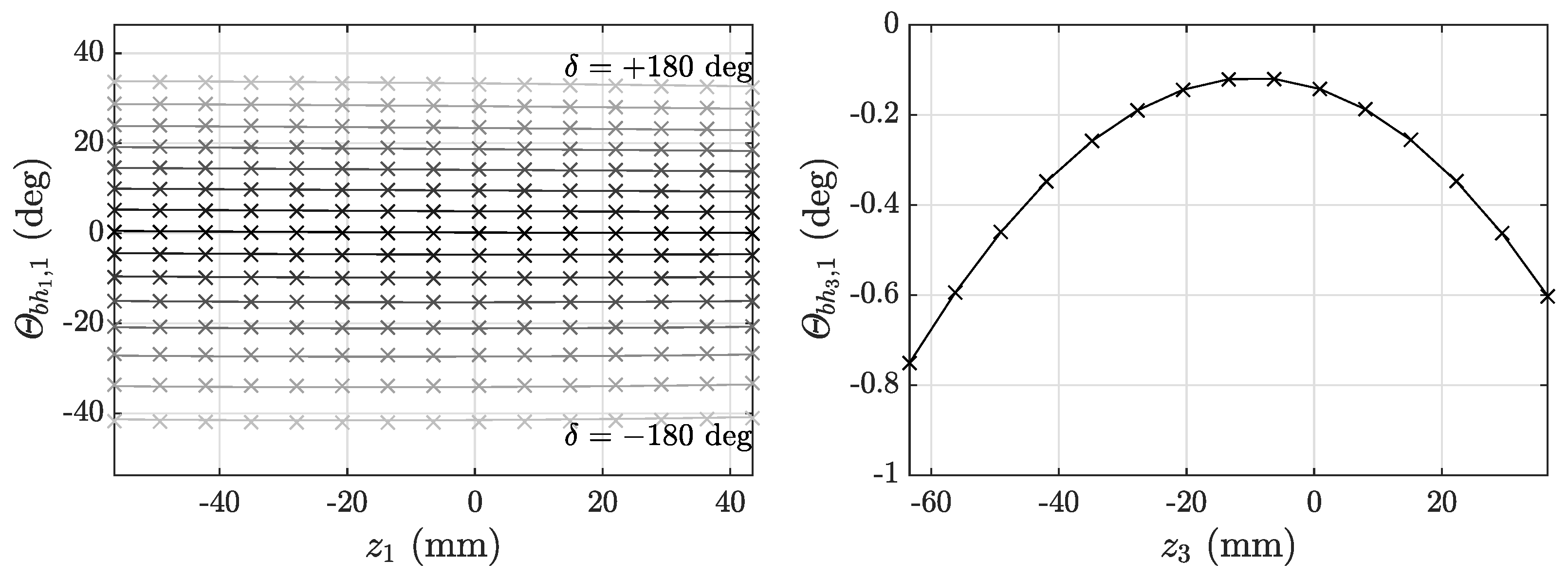As a last step, for each coordinate $q_{bh,i}$, we fit (in the least-squares sense) the corresponding grid of points $q_{bh,i}^{(p,l)}$ with a 2D regression polynomial $q_{bh,i}(z,\delta )$ in the two variables $(z,\delta )$. For our purposes, the following polynomial (complete of order three) turned out to be sufficiently accurate:

$$q_{bh,i}(z,\delta )=\sum _{r=0}^3\sum _{s=0}^{3-r}{a}_{rs,i}{z}^r{\delta }^s.$$

(2)

In Figure 4, the procedure is illustrated for the variable $q_{bh,4}={\Theta }_{bh,1}$ (wheel steer angle). Assembling Equation (2) with (1), we obtain $g_{bh}$ as a function of z and $\delta$, i.e., $g_{bh}\left(q_{bh}(z,\delta )\right)$.

Now we need to relate the rigid-body velocity $V_{bh}$ to the derivatives $\dot{z}$ and $\dot{\delta }$. In the first instance, we write

$$V_{bh}=\sum _{i=1}^6{J}_{bh,i}{\dot{q}}_{bh,i},$$

(3)

where $J_{bh}$ is the geometric Jacobian of the suspension joint relative to $q_{bh}$, assumed with independent components. Each column of $J_{bh}$ can be computed based on the PoE Formula (1), as shown in ([20], Section 3.4). For the i-th column, we have $J_{bh,i}=A_i^{-1}{Y}_i$, with $A_6=I_{6\times 6}$ and $A_i={\mathrm{Ad}}_{e^{{\widehat{Y}}_i{q}_{bh,i}}\cdots e^{{\widehat{Y}}_6{q}_{bh,6}}}$, $i=1,\cdots ,5$. According to ([20], Section 2.4.2), we define the adjoint operator${\mathrm{Ad}}_g$ as the $6\times 6$ matrix satisfying $Y={\mathrm{Ad}}_{g}X$ whenever $\widehat{Y}=g\widehat{X}{g}^{-1}$, so that, if $g=\left[\begin{array}{cc}R& d\\ 0^T& 1\end{array}\right]$, then ${\mathrm{Ad}}_g=\left[\begin{array}{cc}R& \widehat{d}R\\ 0& R\end{array}\right]$.

Since $q_{bh,i}$ is a function of $(z,\delta )$, the velocities of the dependent variables ${\dot{q}}_{bh,i}$ can be expanded using the chain rule

$${\dot{q}}_{bh,i}=\frac{\partial }{\partial z}{q}_{bh,i}\dot{z}+\frac{\partial }{\partial \delta }{q}_{bh,i}\dot{\delta },$$

(4)

where the (geometric) partial derivatives $\frac{\partial }{\partial z}{q}_{bh,i}$ and $\frac{\partial }{\partial \delta }{q}_{bh,i}$ are obtained by differentiating Equation (2). Then, by defining the Jacobians with respect to the true independent variables z and $\delta$ as follows

$$\begin{array}{c}\hfill J_{bh,z}=\sum _{i=1}^6{J}_{bh,i}\frac{\partial }{\partial z}{q}_{bh,i}\mathrm{and}{J}_{bh,\delta }=\sum _{i=1}^6{J}_{bh,i}\frac{\partial }{\partial \delta }{q}_{bh,i},\end{array}$$

(5)

it possible to obtain the rigid-body velocity $V_{bh}$ of the constrained motion from Equation (3), in terms of $\dot{z}$ and $\dot{\delta }$, as follows:

$$V_{bh}=J_{bh,z}\dot{z}+J_{bh,\delta }\dot{\delta }.$$

(6)

In Section 3, we will also need the time derivative ${\dot{V}}_{bh}$ of the rigid-body velocity $V_{bh}$. For this, we need to differentiate Equations (3)–(6). Starting, as before, under the assumptions of independent components $q_{bh}$, by differentiation of (3) we obtain

$${\dot{V}}_{bh}=\sum _{i=1}^6{\dot{J}}_{bh,i}{\dot{q}}_{bh,i}+\sum _{i=1}^6{J}_{bh,i}{\ddot{q}}_{bh,i}.$$

(7)

In (7), following [22], the derivatives ${\dot{J}}_{bh,i}$ can computed using the formula

$$\begin{array}{c}\hfill {\dot{J}}_{bh,i}=-\sum _{i<j\le 6}{\mathrm{ad}}_{J_{bh,j}{\dot{q}}_{bh,j}}{J}_{bh,i}\end{array}$$

(8)

that efficiently exploits Lie derivatives between the columns of $J_{bh}$. (In the matrix case, we compute the Lie derivative of the vector field $\widehat{X}$ with respect to vector field $\widehat{Y}$ by using the commutator $\widehat{Z}=\widehat{Y}\widehat{X}-\widehat{X}\widehat{Y}$; in the vector case, we use the $6\times 6$ matrix ${\mathrm{ad}}_Y$, defined such that $Z={\mathrm{ad}}_{Y}X$. If v and $\omega$ are the translational and rotational component of V, then ${\mathrm{ad}}_V=\left[\begin{array}{cc}\widehat{\omega }& \widehat{v}\\ 0& \widehat{\omega }\end{array}\right]$.)

In (7), the accelerations ${\ddot{q}}_{bh,i}$ are obtained by differentiating the velocities in Equation (4):

$${\ddot{q}}_{bh,i}=\frac{{\partial }^2}{\partial z^2}{q}_{bh,i}{\dot{z}}^2+2\frac{{\partial }^2}{\partial z\partial \delta }{q}_{bh,i}\dot{z}\dot{\delta }+\frac{{\partial }^2}{\partial {\delta }^2}{q}_{bh,i}{\dot{\delta }}^2+\frac{\partial }{\partial z}{q}_{bh,i}\ddot{z}+\frac{\partial }{\partial \delta }{q}_{bh,i}\ddot{\delta },$$

(9)

where the (geometric) partial derivatives are obtained by differentiating the polynomials in (2). At this point, we have explicit expressions for the derivatives of the Jacobians in (5) which are

$$\begin{array}{cc}\hfill {\dot{J}}_{bh,z}& =\sum _{i=1}^6{\dot{J}}_{bh,i}\frac{\partial }{\partial z}{q}_{bh,i}+\sum _{i=1}^6{J}_{bh,i}\left(\frac{{\partial }^2}{\partial z^2}{q}_{bh,i}\dot{z}+\frac{{\partial }^2}{\partial z\partial \delta }{q}_{bh,i}\dot{\delta }\right)\mathrm{and}\hfill \end{array}$$

(10)

$$\begin{array}{cc}\hfill {\dot{J}}_{bh,\delta }& =\sum _{i=1}^6{\dot{J}}_{bh,i}\frac{\partial }{\partial \delta }{q}_{bh,i}+\sum _{i=1}^6{J}_{bh,i}\left(\frac{{\partial }^2}{\partial z\partial \delta }{q}_{bh,i}\dot{\delta }+\frac{{\partial }^2}{\partial {\delta }^2}{q}_{bh,i}\dot{\delta }\right).\hfill \end{array}$$

(11)

By substituting Equations (8) and (9) in (7), and casting some intermediate results as (10) and (11), we have explicit expressions for computing the constrained rigid-body acceleration ${\dot{V}}_{bh}$ in the following form:

$${\dot{V}}_{bh}={\dot{J}}_{bh,z}\dot{z}+{\dot{J}}_{bh,\delta }\dot{\delta }+J_{bh,z}\ddot{z}+J_{bh,\delta }\ddot{\delta }.$$

(12)

The last step in our analysis is aimed at characterizing the generalized force $\tau \in \mathbb{R}$ of the suspension associated with the independent configuration variable $z\in \mathbb{R}$. We assume that $\tau$ is entirely due to the force developed by a shock absorber consisting of a spring and damper aligned along the same axis. The intensity F of this force is a function of the length l of the spring and its derivative $\dot{l}$ as follows:

$$F=k_s(l-l_0)+c_d\dot{l}$$

(13)

(a linear behavior for both the spring and the damper is assumed). Independently of the complexity of the kinematics leading to the shock absorber, the length l of the spring ultimately depends on the suspension configuration. To find l as a function of z (and possibly $\delta$), we solve the linkage kinematics for l at a number of predetermined configurations, and then fit the samples with a regression polynomial similar to (2). Then, by employing the principle of virtual work, $\tau$ can be computed as

$$\tau \delta z=F\delta l\Rightarrow \tau =F\frac{\partial l}{\partial z}$$

(14)

In (14), F is evaluated using l and $\dot{l}=\frac{\partial l}{\partial z}\dot{z}$, which are computed using the regression polynomial and its derivative. In this way, we have $\tau$ expressed as a function of z and $\dot{z}$, i.e., $\tau =\tau (z,\dot{z})$. We will need this in Section 3.

2.3. Tire Model

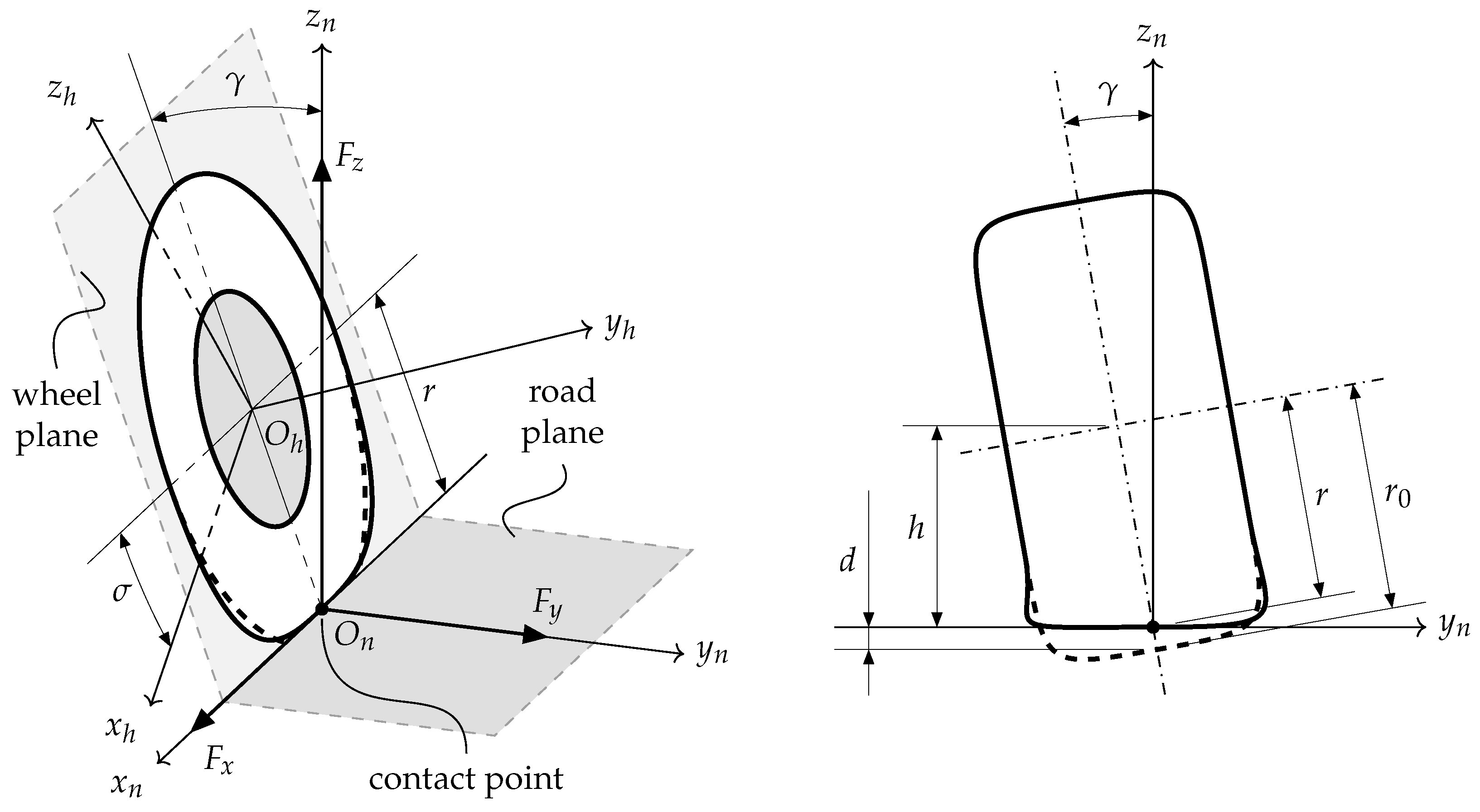
The tire model is responsible for all forces exchanged with the ground and, as such, is a fundamental component of the vehicle. To conveniently define the tire forces we introduce, for each wheel, an auxiliary reference frame $\left\{N\right\}$. The construction of the frame $\left\{N\right\}$ is illustrated in Figure 5. Note that frame $\left\{N\right\}$ is completely specified given the pose of the knuckle frame $\left\{H\right\}$ and that of the current track frame $\left\{S\right\}$.

The tire force is decomposed into three orthogonal components, $F_x,F_y,F_z$, aligned, respectively, with the axes of $\left\{N\right\}$, as shown in Figure 5 (left panel). To compute the vertical force $F_z$, we use a unilateral penalty-based compliant tire model, where the tire is modeled as a radial spring, with uniform radial stiffness $k_t$. The normal force arises whenever the pose of $\left\{H\right\}$ is such that the lowermost point of the undeformed tire (in fact, of its longitudinal section; see Figure 5 (right panel)) is displaced below the road surface. We denote the amount of this displacement by d, and let $F_z$ be proportional to d as follows:

$$F_z=\left\{\begin{array}{cccc}& k_{t}d\hfill & \hfill & \mathrm{if}d>0\hfill \\ & 0\hfill & \hfill & \mathrm{if}d\le 0.\hfill \end{array}\right.$$

(15)

When the tire is completely detached from ground, the vertical force $F_z$ is set to zero. In this way, we are able to correctly deal with tires losing contact with ground, e.g., during a jump.

To compute the value of the tangential forces $F_x$ and $F_y$, we rely on Pacejka’s Magic Formula ([16], Section 4.3.2):

$$[F_x,F_y]=mf(\kappa ,\alpha ,F_z,\gamma ).$$

(16)

The Magic Formula, mf, computes the longitudinal and lateral forces $F_x,F_y$ as a function of the tire slips$\kappa ,\alpha$ ([16], Section 1.2.1). The formula is also sensitive to variations of vertical load $F_z$ and camber angle $\gamma$.

2.4. External Wrenches

In this section we detail the contributions of all forces exchanged by the environment and the vehicle. For each body, we compute the resultant external wrench and express it in the local reference frame.

The resultant external wrench $W_{we}$ applied to the generic rim expressed in the knuckle frame $\left\{H\right\}$ is

$$W_{we}={\mathrm{Ad}}_{g_{hn}}^{\ast }{W}_t+W_d+W_b+W_{w_h},$$

(17)

and is made of four contributions. The first is due to the tire forces $W_t={[F_x,F_y,F_z,0,0,0]}^T$ with components in $\left\{N\right\}$ defined in Section 2.3. Their expression in $\left\{H\right\}$ can easily be computed through the coadjoint operator ${\mathrm{Ad}}_{g_{hn}}^{\ast }={\mathrm{Ad}}_g^{-T}$. The second and third contributions $W_d$ and $W_b$, respectively, are due to the relative driving $T_d$ and braking torque $T_b$, and are applied to the wheel around the hub axis $y_h$. In frame $\left\{H\right\}$, their explicit expressions are therefore $W_d={[0,0,0,0,T_d,0]}^T$ and $W_b={[0,0,0,0,T_b,0]}^T$. It should be noted, however, that although both $T_d$ and $T_b$ are applied about the same axis $y_h$, the reaction of the former goes to the chassis (through the drive axle), whereas that of the latter goes to the knuckle (through the brakes). Therefore, we prefer to introduce these torques, together with their respective reactions, as ordinary external torques, and keep the joint torque of the hub bearing always set to zero. The magnitude of $T_d$ and $T_b$ is determined starting from a single input signal T, which is interpreted as a driving/braking command depending on its positive/negative sign. In this way, simultaneous acceleration and braking is disallowed. Denoting the positive and negative value of T by $T_{+}$ and $T_{-}$, we define

$$T_d=\left\{\begin{array}{cccc}& 0\hfill & \hfill & \mathrm{if}k=1,2\hfill \\ \hfill & \frac{T_{+}}{2}\hfill & \hfill & \mathrm{if}k=3,4\hfill \end{array}\right.\mathrm{and}{T}_b=\left\{\begin{array}{cccc}\hfill & k_b\frac{T_{-}}{2}\hfill & \hfill & \mathrm{if}k=1,2\hfill \\ \hfill & (1-k_b)\frac{T_{-}}{2}\hfill & \hfill & \mathrm{if}k=3,4\hfill \end{array}\right.$$

(18)

The driving torque $T_d$ is computed assuming a rear-wheel-drive vehicle with an open differential. The braking torque $T_b$, on the other hand, is computed by partitioning the total braking torque $T_{-}$ between front and rear axle according to the value of the brake balance coefficient $k_b$, specified in the car set-up.

The last contribution $W_{w_h}$ in (17) is due to the weight force of each wheel (rim + tire), expressed in frame $\left\{H\right\}$. Its general expression is of the form $W_{w_h}={[F_{w_h}^T{R}_{hg}^T,0,0,0]}^T$, with $F_{w_h}={[0,0,-m_{h}g]}^T$ in frame $\left\{G\right\}$.

The external wrench $W_{he}$ applied to the knuckles is simply given by the reaction of the braking torque $W_b$, thus

$$W_{he}=-W_b.$$

(19)

Finally, we define the resultant external wrench $W_{be}$ applied to the chassis expressed in $\left\{B\right\}$ frame as follows:

$$W_{be}=W_a-{\mathrm{Ad}}_{g_{bh}}^{\ast }{W}_d+W_{w_b}.$$

(20)

In (20) we recognize three contributions. The first one is the aerodynamic wrench $W_a$ which, following ([9], Section 3.7.2), is decomposed into drag and lift components so that $W_a=-\frac{1}{2}\rho S{v}_{gb,1}^2{[C_x,0,C_z,0,-h_0{C}_x-a_f{C}_{zf}+a_r{C}_{zr},0]}^T$. Here, $\rho$ is the air density, S the frontal area of the vehicle, $v_{gb,1}$ the forward velocity, $h_0$ the nominal height of the CoM from ground, and $a_f,a_r$ the distances of the CoM from the front and rear axle. The drag and lift coefficients $C_x$ and $C_z$ are dimensionless parameters that depend on the shape of the vehicle’s body. $C_z$ can be further partitioned into $C_{zf}=k_a{C}_z$ and $C_{zr}=(1-k_a)C_z$ according to the aerodynamic balance coefficient$k_a$, which is a parameter of the vehicle set-up. The second contribution in (20) is the reaction of the driving torque $W_d$, conveniently transformed into frame $\left\{B\right\}$.

The last contribution $W_{w_b}$ is the own weight of the chassis in $\left\{B\right\}$. Its general expression is of the form $W_{w_b}={[F_{w_b}^T{R}_{bg}^T,0,0,0]}^T$, with $F_{w_b}={[0,0,-m_{b}g]}^T$ in frame $\left\{G\right\}$.

3. Vehicle Dynamics

In this section we derive the equations of motion governing our articulated system. Ultimately, we will be able to express the system dynamics in the classical state-space form as follows:

$$\dot{x}=f(x,u).$$

(21)

In this way, the dynamical equations are ready to be embedded into our MLTP formulation.

As state variables, we take the velocity and position variables defined in Section 2.1. More explicitly, our state vector is $x=(q_{gb};V_{gb};z;\dot{z};\omega )\in {\mathbb{R}}^{24}$. Here, $q_{gb}\in {\mathbb{R}}^6$ collects the Cartesian coordinates and Euler ZYX angles of the chassis with respect to the inertial frame $\left\{B\right\}$, $V_{gb}\in {\mathbb{R}}^6$ is its distal rigid-body velocity, $z\in {\mathbb{R}}^4$ collects the four suspension travels, $\dot{z}\in {\mathbb{R}}^4$ their derivatives, and $\omega \in {\mathbb{R}}^4$ the speeds of the four wheels. As control input, we take $u=(T,\delta )\in {\mathbb{R}}^2$, where we cast the driving/braking torque T and the steering wheel angle $\delta$ (for optimization purposes, we shall omit the contributions of $\dot{\delta }$ and $\ddot{\delta }$).

To compute the derivative of the state vector $\dot{x}$, we start by noting that, given $V_{gb}$, the derivatives ${\dot{q}}_{gb}$ are readily obtained as

$${\dot{q}}_{gb}=J_{gb}^{-1}\left(q_{gb}\right)V_{gb},$$

(22)

where $J_{gb}\left(q_{gb}\right)\in {\mathbb{R}}^{6\times 6}$ is the geometric Jacobian of the virtual six-DoF joint connecting $\left\{B\right\}$ to $\left\{G\right\}$. The matrix $J_{gb}$ is systematically computed through a PoE parameterization of the transformation $g_{gb}$, in analogy to what has been carried out for $J_{bh}$ in Equation (3). No further consideration is here necessary, since $q_{gb}$ have independent components.

We now need to find the derivatives of the velocity variables, ${\dot{V}}_{gb},\ddot{z},\dot{\omega }$. For this, the equations for the motion of the vehicle must be formulated. We rely, for this task, on a computational method inspired by the articulated-body algorithm (ABA) by Featherstone ([12], Section 7.2). The key concept of the approach is that of an articulated body: its inertia is that of the original parent rigid body, plus the portion of the sub-tree (of the children bodies) which can be structurally transmitted backward to the parent through the joints. This allows us to build the equations of motion recursively and in such a way that, in the end, one can obtain explicitly (non matrix inversion is required) the acceleration of each body decoupled from the others. Besides being compact and systematic, the process also presents clear computational advantages.

To adapt the ABA to the case of our vehicle, some observations about the basic features of the system are in order. First and foremost is that the chassis $\left\{B\right\}$ (root of the kinematic tree), is a free-floating body in the inertial reference frame $\left\{G\right\}$: its rigid-body acceleration ${\dot{V}}_b$ is not available as external and independent information, but is the result of the motion of the other bodies of the system, ultimately depending on the wrenches $W_{we}$, $W_{he}$, and $W_{be}$ exchanged with the external environment by it and its children bodies. Another complication is that, as detailed in Section 2, the one-DoF suspension joints connecting $\left\{B\right\}$ to $\left\{H\right\}$ are not merely revolute or prismatic, but are complex joints whose motion subspaces depend on their current configuration, ultimately encoded in z. Moreover, at the front wheels, the suspension joints are not only configuration-dependent with respect to z, but also time-varying joints (through the control input $\delta \left(t\right)$ and its derivatives). A way to tackle all these issues is shown following the steps of the ABA in the remainder of this section.

In Algorithm 1, rigid-body velocities are propagated forward across the nodes of the kinematic tree in Figure 3 from the root node to the leaves. (In the pseudo-code Algorithms 1 and 2, the articulated inertia and bias, ${\widehat{M}}_i$ and ${\widehat{B}}_i$, are expressed in the same reference frame as the respective rigid-body velocity $V_i$, for $i=b,h,w$.) Starting with the rigid-body velocity $V_b$ of the chassis $\left\{B\right\}$, which is directly available from the state vector x, the computation of the rigid-body velocity is propagated first to the knuckles $\left\{H\right\}$ and then to the rims $\left\{W\right\}$. The relative rigid-body velocities $V_{bh}$ realized by the suspension are computed according to Equation (6), using the joint velocities $\dot{z}$ and $\dot{\delta }$ together with the Jacobians $J_{bh,z}$ and $J_{bh,\delta }$ defined in Equation (5). (Note that, for a front-wheel-steering vehicle, the contribution relative to $\delta$ is null at the rear wheels.) To compute the relative rigid-body velocities $V_{hw}$ realized by the hub bearings, we use the wheel speeds $\omega$ together with the (constant) Jacobian $J_{hw}={[0,0,0,0,1,0]}^T$, that represents the screw coordinates of the hub axis.

Algorithm 1 Forward Propagation of Velocity

1: for $h=h_1,h_2,h_3,h_4$ do   2:     $V_{bh}=J_{bh,z}\dot{z}+J_{bh,\delta }\dot{\delta }$   3:     $V_h={\mathrm{Ad}}_{g_{bh}}^{-1}{V}_b+V_{bh}$        ▹ Knuckle Rigid-Body Velocity   4:     $V_{hw}=J_{hw}\omega$   5:     $V_w=V_h+V_{hw}$            ▹ Rim Rigid-Body Velocity   6: end for

Algorithm 2 Backward Propagation of Articulated Inertia and Bias

1: for $h=h_1,h_2,h_3,h_4$ do    2:     ${\widehat{M}}_w=M_w$                      ▹ Rim Articulated Inertia    3:     ${\widehat{B}}_w=-W_{we}+{\mathrm{ad}}_{V_w}^{\ast }{M}_w{V}_w$               ▹ Rim Articulated Bias    4:     ${\overline{M}}_w={\widehat{M}}_w-{\displaystyle \frac{{\widehat{M}}_w{J}_{hw}{J}_{hw}^T{\widehat{M}}_w}{J_{hw}^T{\widehat{M}}_w{J}_{hw}}}$    5:     ${\overline{B}}_w={\widehat{B}}_w-{\displaystyle \frac{{\widehat{M}}_w{J}_{hw}{J}_{hw}^T{\widehat{B}}_w}{J_{hw}^T{\widehat{M}}_w{J}_{hw}}}-{\overline{M}}_w{\mathrm{ad}}_{V_{hw}}{V}_w$    6:     ${\widehat{M}}_h={\overline{M}}_w$                     ▹ Knuckle Articulated Inertia    7:     ${\widehat{B}}_h=-W_{he}+{\overline{B}}_w$                    ▹ Knuckle Articulated Bias  8:     ${\overline{M}}_h={\widehat{M}}_h-{\displaystyle \frac{{\widehat{M}}_h{J}_{bh,z}{J}_{bh,z}^T{\widehat{M}}_h}{J_{bh,z}^T{\widehat{M}}_h{J}_{bh,z}}}$    9:     ${\overline{B}}_h={\widehat{B}}_h-{\displaystyle \frac{{\widehat{M}}_h{J}_{bh,z}(J_{bh,z}^T{\widehat{B}}_h-\tau )}{J_{bh,z}^T{\widehat{M}}_h{J}_{bh,z}}}-{\overline{M}}_h({\mathrm{ad}}_{V_{bh}}{V}_h-{\dot{J}}_{bh,z}\dot{z}-{\dot{J}}_{bh,\delta }\dot{\delta }-J_{bh,\delta }\ddot{\delta })$   10: end for  11: ${\displaystyle {\widehat{M}}_b=M_b+\sum _h{\mathrm{Ad}}_{g_{bh}}^{\ast }{\overline{M}}_h{\mathrm{Ad}}_{g_{bh}}^{-1}}$            ▹ Chassis Articulated Inertia   12: ${\displaystyle {\widehat{B}}_b=-W_{be}+{\mathrm{ad}}_{V_b}^{\ast }{M}_b{V}_b+\sum _h{\mathrm{Ad}}_{g_{bh}}^{\ast }{\overline{B}}_h}$         ▹ Chassis Articulated Bias

The chassis velocity $V_b$ is transformed into $\left\{H\right\}$ via the (inverse of the) adjoint operator

$${\mathrm{Ad}}_{g_{bh}}=\left[\begin{array}{cc}{R}_{bh}& {\widehat{d}}_{bh}{R}_{bh}\\ 0& R_{bh}\end{array}\right],$$

(23)

where $g_{bh}$ is computed as a function of z (and $\delta$), as shown in Section 2.2. Since for the rims we use the same reference frame as the knuckles, no adjoint transformation is needed between $\left\{H\right\}$ and $\left\{W\right\}$ quantities.

In Algorithm 2, we compute the articulated inertia $\widehat{M}$ and bias force $\widehat{B}$ of each body. According to [12], the articulated inertia $\widehat{M}$ is the inertia that a body appears to have when it is part of an articulated system of bodies. The articulated bias force $\widehat{B}$ is defined instead as the value that the resultant wrench W applied by the parent node on the tree should take in order for the rigid-body acceleration $\dot{V}$ of a body to be null. Using the concepts of articulated inertia and bias, the Newton–Euler equation for the generic articulated body can be written in the form

$$W=\widehat{M}\dot{V}+\widehat{B}.$$

(24)

For a leaf node of the kinematic tree, the articulated inertia $\widehat{M}$ is the generalized inertia matrix of the body M itself. Accordingly, the articulated bias $\widehat{B}$ reduces to

$$B=-W_e+{\mathrm{ad}}_V^{\ast }MV,$$

(25)

where $W_e$ is the resultant external wrench applied to the body and ${\mathrm{ad}}_V^{\ast }MV$ accounts for the generalized gyroscopic and centrifugal forces, which are bi-linear in V. According to ([20], Section 4.3.3), we defined ${\mathrm{ad}}_V^{\ast }=-{\mathrm{ad}}_V^T$. (If v and $\omega$ are the translational and rotational component of V, then ${\mathrm{ad}}_V^{\ast }=\left[\begin{array}{cc}\widehat{\omega }& 0\\ \widehat{v}& \widehat{\omega }\end{array}\right]$.)

In the case of our vehicle, the leaf nodes are the rims $\left\{W\right\}$ (see Figure 3). Once their inertia and bias are initialized as ${\widehat{M}}_w$ and ${\widehat{B}}_w$, the standard ABA equations are applied, as illustrated in [12], to compute the articulated inertia and bias of the knuckles $\left\{H\right\}$ (parent of each leaf) as ${\widehat{M}}_h$ and ${\widehat{B}}_h$. The process is then repeated to get the articulated inertia and bias of the chassis $\left\{B\right\}$ (root of our kinematic tree) as ${\widehat{M}}_b$ and ${\widehat{B}}_b$.

To successfully back-propagate articulated inertias and bias forces, we must provide the algorithm with the necessary information about the external forces, the geometry of the joints, the mass distribution of the bodies, as well as their current state of motion. In this respect, we observe that the rigid-body velocities $V_b,V_h,V_w$ are known from Step 1. Under our simplifying assumptions that $M_h=0$, the chassis and the rims are the only bodies provided with non-null mass distribution; their inertia matrices $M_b$ and $M_w$ are given and constant and are expressed in the reference frames $\left\{B\right\}$ and $\left\{H\right\}$, respectively. As far as the external forces are concerned, the wrenches $W_{be}$, $W_{he}$ and $W_{we}$ are computed according to Equation (17), (19), and (20). Finally, to capture the geometry of the motion allowed by the joints, we use again the Jacobians $J_{hw}$ as well as $J_{bh,z}$, and $J_{bh,\delta }$ from Equation (5) and their derivatives ${\dot{J}}_{bh,z}$ and ${\dot{J}}_{bh,\delta }$ from (10). The generalized suspension forces $\tau$, which account for the transmission of the actions from the knuckles to the chassis through the springs and dampers, are computed using Equation (14).

In Algorithm 3, the algorithm outputs the derivatives of the velocity variables, ${\dot{V}}_b$, $\ddot{z}$ and $\dot{\omega }$. To obtain ${\dot{V}}_b$, we solve the Newton–Euler equation (24) for the acceleration of the chassis articulated body. The left-hand side is zero, since the chassis is free-floating with respect to the inertial reference frame, meaning no wrench is exerted by the virtual six-DoF joint. Knowing ${\dot{V}}_b$, we can then calculate the suspension travel accelerations $\ddot{z}$ by projecting the Newton–Euler equation of the knuckle along the direction of $J_{bh,z}$ and solving for $\ddot{z}$. With $\ddot{z}$, we can calculate the rigid-body acceleration ${\dot{V}}_h$ of the knuckle. The knowledge of ${\dot{V}}_h$ is necessary to compute the wheel angular accelerations $\dot{\omega }$, using a similar procedure as for $\ddot{z}$.

Algorithm 3 Forward Propagation of Acceleration

1: ${\dot{V}}_b=-{\widehat{M}}_b^{-1}{\widehat{B}}_b$                 ▹ Chassis Rigid-Body Acceleration   2: for $h=h_1,h_2,h_3,h_4$ do   3:     $\ddot{z}=-{\displaystyle \frac{J_{bh,z}^T\left({\widehat{B}}_h+{\widehat{M}}_h({\mathrm{Ad}}_{g_{bh}}^{-1}{\dot{V}}_b-{\mathrm{ad}}_{V_{bh}}{V}_h+{\dot{J}}_{bh,z}\dot{z}+{\dot{J}}_{bh,\delta }\dot{\delta }+J_{bh,\delta }\ddot{\delta })\right)-\tau }{J_{bh,z}^T{\widehat{M}}_h{J}_{bh,z}}}$   4:     ${\dot{V}}_{bh}={\dot{J}}_{bh,z}\dot{z}+{\dot{J}}_{bh,\delta }\dot{\delta }+J_{bh,z}\ddot{z}+J_{bh,\delta }\ddot{\delta }$   5:     ${\dot{V}}_h={\mathrm{Ad}}_{g_{bh}}^{-1}{\dot{V}}_b-{\mathrm{ad}}_{V_{bh}}{V}_h+{\dot{V}}_{bh}$        ▹ Knuckle Rigid-Body Acceleration   6:     $\dot{\omega }=-{\displaystyle \frac{J_{hw}^T\left({\widehat{B}}_w+{\widehat{M}}_w({\dot{V}}_h-{\mathrm{ad}}_{V_{hw}}{V}_w)\right)}{J_{hw}^T{\widehat{M}}_w{J}_{hw}}}$   7: end for

We have finished describing the three steps of the articulated-body algorithm, which, along with Equation (22), are crucial components of our state transition function $f(·)$ in Equation (21). It is important to note that $f(·)$ relies on numerous parameters, including both constant and time-varying data. The constant data include all the dimensions, coefficients, and parameters utilized in the model’s creation. On the other hand, the time-varying data pertain to the coordinates of the track frame S (specifically, the Cartesian coordinates $g_{gs}$ and the Euler ZYX angles ${\Phi }_{gs}$), which are required to compute the external wrenches in Equations (17), (19) and, (20). It is the presence of the latter that causes the state transition function to become a time-varying function.

4. Minimum-Lap-Time Planning

In this section, the dynamic vehicle model developed so far is embedded into a minimum-lap-time optimization problem. Before delving into the details of our formulation and implementation, however, we point out that the modeling approach proposed in this article does not impose any particular solution method, and can possibly be used within different optimization frameworks.

4.1. Formulation via Direct Collocation

The optimization approach proposed in this article involves recasting the MLTP, originally formulated as an optimal control problem, into a nonlinear program via a direct collocation technique. The resulting NLP has the form

$$\begin{array}{cc}\hfill \underset{x,v,u,z}{\mathrm{minimize}}& \sum _{k=1}^N{L}_k(x_k,v_k,u_k,z_k)\hfill \end{array}$$

(26)

$$\begin{array}{cc}\hfill \mathrm{subject}\mathrm{to}& g_k(x_{k-1},x_k,v_k,u_k,z_k)=0,k=1,\dots ,N,\hfill \end{array}$$

(27)

$$\begin{array}{cc}\hfill & h_k(x_k,u_k,z_k)\le 0,k=1,\dots ,N.\hfill \end{array}$$

(28)

To perform discretization, we parameterize the track centerline with a curvilinear abscissa $\alpha \in [0,1]$, and we sample its domain at $N+1$ points ${\alpha }_0,\dots ,{\alpha }_N$. To each sample ${\alpha }_k$, we associate the track frame $\left\{S_k\right\}$ whose origin coincides with the point on the track centerline corresponding to ${\alpha }_k$, as shown in Figure 6. We know everything about this frame, and we are able to get all information we desire. Most importantly, all this information can be extracted and pre-processed off-line.

Following the direct collocation approach, the state trajectory on the k-th step of the grid is approximated with a polynomial $p_k$. The polynomial is defined on the unit interval and then scaled to match the width $h_k$ of the corresponding time step. On the unit interval, we select d collocation points ${\tau }_1,\dots ,{\tau }_d$, associated with as many collocation states $v_{k,1},\dots ,v_{k,d}$. In order to ensure compliance between the polynomial trajectory and the system dynamics (21) we enforce, at each collocation point, the equality constraint:

$$\frac{1}{h_k}\frac{\partial }{\partial \tau }{p}_k\left({\tau }_i\right)=f(v_{k,i},u_k).$$

(29)

where $f(·)$ is evaluated using the track data relative to $\left\{S_k\right\}$ we already have at our disposal. The step size $h_k$ is included among the auxiliary variables $z_k$ which appear, along with the states $x_k$, collocation states $v_k$, and inputs $u_k$, as decision variables of the NLP.

Besides Equation (29), the equality constraints in (27) include additional conditions that take care of the continuity between the polynomial pieces.

The inequality constraints in (28) include instead all path constraints limiting the value of the decision variables. We also exploit the constraints in (28) to enforce the vehicle to stay on track; specifically, we want not only to prevent it from going off track sideways, but we want it to interact with the track frame $\left\{S_k\right\}$ we are actually using at the k-th grid point. (For this, we require that the chassis CoM lies on the $yz$-plane of the track frame.)

Regarding the cost functional in (26), within a minimum-lap-time problem, a possible expression for the running cost $L_k$ may be

$$L_k=h_k^2+k_{\delta }{({\delta }_k-{\delta }_{k-1})}^2+k_T{(T_k-T_{k-1})}^2,$$

(30)

where the first term penalizes the total lap-time (sum of the $h_k$’s) and the last two contributions serve to prevent abrupt variations of the control inputs.

4.2. Implementation Details

To perform the transcription operations, we used the tools provided by CasADi [23], an open-source library that provides tools for formulating and solving large-scale optimization problems, such as the one at hand. CasADi accepts source code as input and stores its operations in the form of computational graphs. These graphs can be evaluated either symbolically or numerically, and automatic differentiation can be efficiently performed on them. We use these graphs to define the objective and constraints of the nonlinear program. The working of CasADi is perfectly suited for taking advantage of sparsity in a problem, which makes it the perfect tool for implementing the large and sparse problem resulting from the direct collocation transcription method. Another plus of CasADi is that it allows a great flexibility in the problem formulation, without imposing a predetermined solver or solution method. For our problem, we used CasADi in combination with the IPOPT [24] solver, which implements the interior-point method.

5. Validation and Results

In this section we report the solution of a MLTP problem with data from a real racetrack. The optimization is carried out on the Nürburgring Nordschleife circuit for a Formula SAE car. To help visualize the outcome of the experiment, we set up an animation and made it available online [25].

To validate the results, the optimal solution found with the proposed model is compared with that obtained by running a double-track model on the same scenario. The double-track model is well established in the vehicle dynamics literature (see, e.g., [9], Section 7.3). Being simple and efficient, it is a useful device to capture the gross motion of the vehicle. On the other hand, the proposed approach is useful for more in-depth analyses of the effects relative to higher-order dynamics offered by our full-fledged multibody model. Compared to the double-track model, the ABA model features: (i) exact rigid-body motion of the chassis, (ii) independent motion of the wheels, (iii) detailed kinematic model of the suspension, (iv) dynamic load transfers accounting also for chassis motion, and (v) dynamic effects induced by traveling along a 3D track with appreciable variations in slope and banking.

Of course, this greater level of detail comes at the expense of a higher computation time. The dimension of the NLP resulting from the ABA-based approach is double compared to that of the double-track. To instantiate the problem, we consider a sector of the circuit with approximately 2 km length. With the proposed ABA-based approach, the NLP comprises 156,000 decision variables and takes 15 min to be solved. With the double-track, we have 78,000 variables and a computation time of 3 min on the same hardware (Simulations were carried out using a 2.30 GHz Intel(R) Core(TM) i7-10875H CPU laptop with 32 GB RAM).

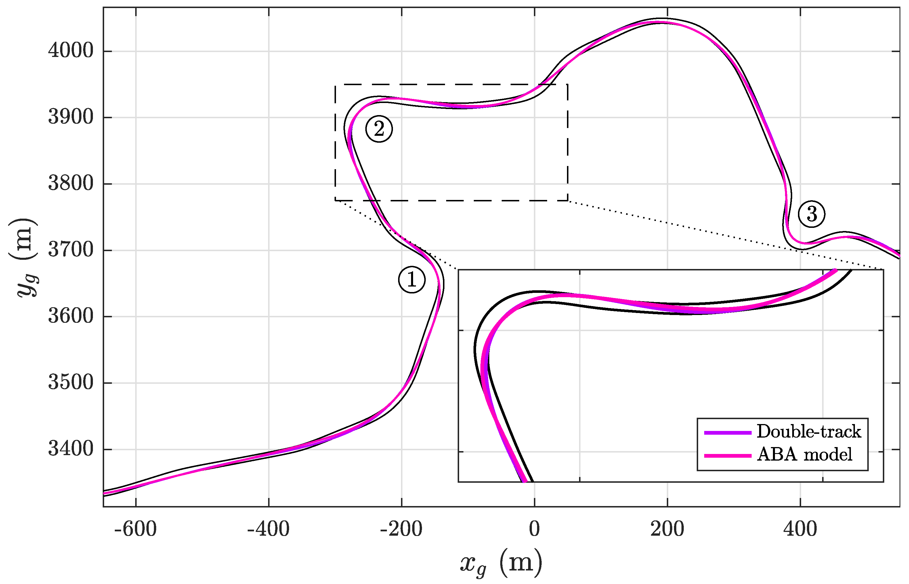
In Figure 7, we report the racing lines obtained by the classic double-track and the proposed ABA-based approach (light and dark red lines, respectively). The main differences can be ascribed to higher-order dynamics elicited in the ABA model by the 3D features of the track, which are not fully captured by the double-track model.

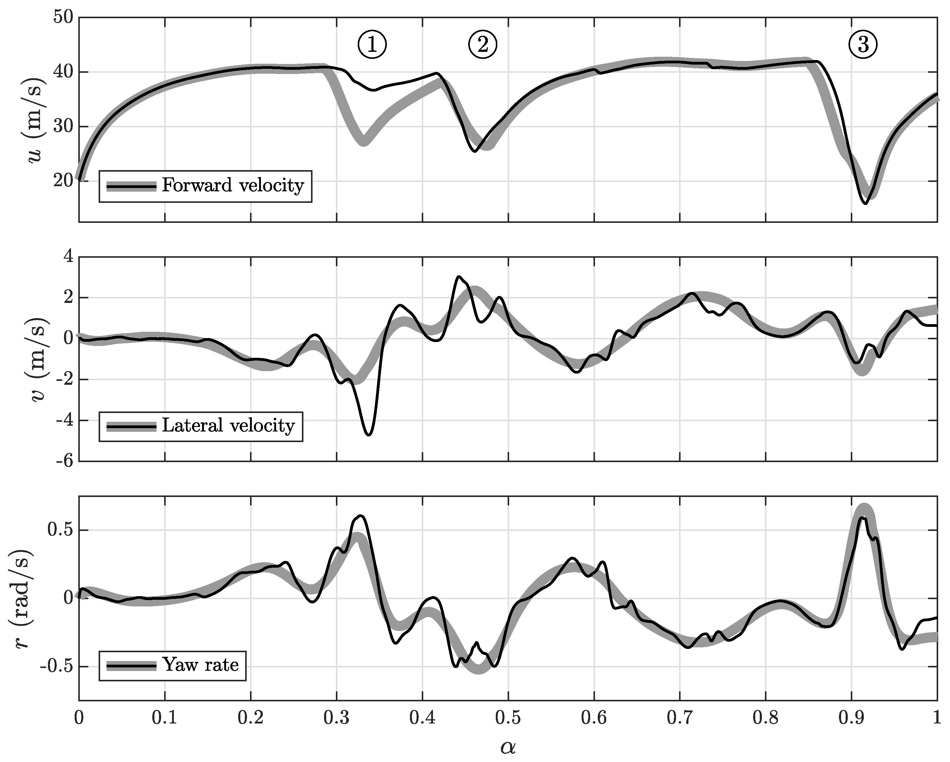
Figure 8 shows the trajectories of the most relevant components of the state vector. The forward velocity $v_{gb,1}$, the lateral velocity $v_{gb,2}$ and the yaw rate ${\omega }_{gb,3}$ are plotted for both the double-track and the proposed ABA model. The trajectories of the former, which appear smoother, are plotted with a shaded line in the background whereas those of the latter are plotted with a solid line in the foreground. Overall, we observe that our ABA model essentially follows the trend defined by the double track; on top of that, it features a richer dynamical presence, which becomes particularly evident in correspondence to sharp corners and highly sloped points of the track.

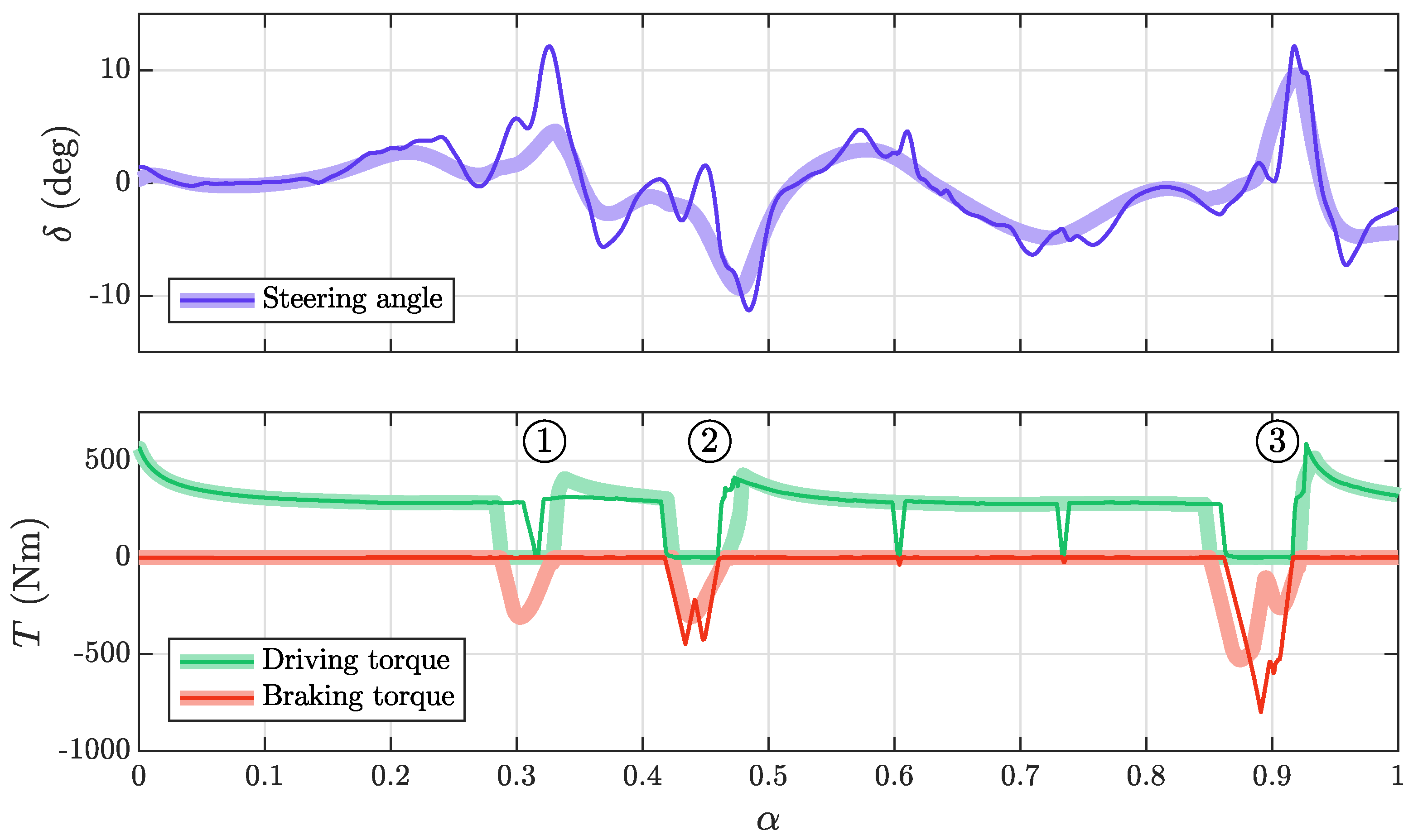
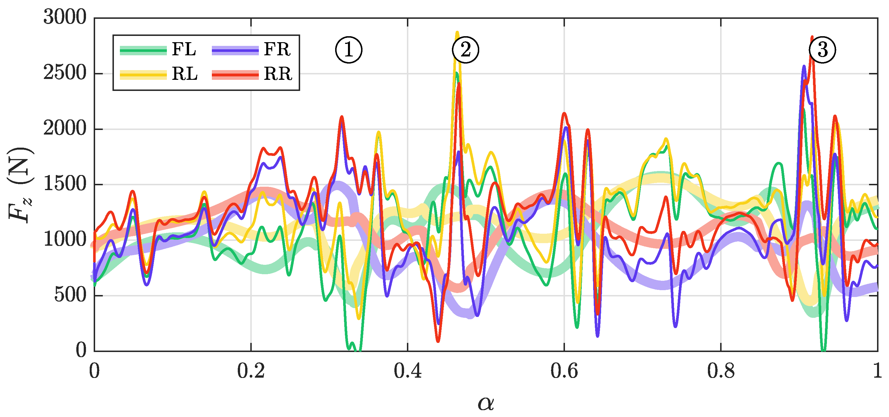
The input trajectories in Figure 9 also follow the same trend. The only appreciable difference between the two models is recorded near corner ①, which the ABA model manages to travel at a higher speed. In fact, this different behavior is reasonable and denotes a peculiarity of our approach. As we point out in the description of Figure 10, the ABA-based planner takes full advantage of the 3D nature of the track to attain a smaller lap-time (57.1 s against the 58.4 s of the double-track). In the particular case of corner ①, the favorable banking and slope angles of the track allow higher vertical loads leading to a sharper negotiation of the corner.

6. Conclusions

In this paper, we presented an approach based on the articulated-body algorithm to derive the dynamic equations of a multibody vehicle model amenable to minimum-lap-time planners. We tackled the 3D nature of the problem in its full extension, making no restrictive assumptions on the mechanics of the system and describing it with rigorous dynamical equations. For the solution of the MLTP, we employed a direct-collocation method, discretizing the problem so that all information of the 3D track was pre-processed and then embedded into the discrete formulation directly. This turned out to be perfectly compatible with our modeling approach, and enabled optimal solutions within accessible computational time frames to be obtained. Given the high level of detail and complexity of the model, we found the proposed approach most useful for in-depth vehicle dynamics analyses on complex tracks.

To substantiate the analysis and assess its validity, we simulated the model of a Formula SAE car on a sector of the Nürburgring Nordschleife circuit, and we provided a detailed comparison with the baseline results provided by a similar MLTP based on the more conventional double-track model. Overall, we observed that the proposed ABA approach agrees, on average, with the trend defined by the double-track model. Noticeably, it features a richer dynamical content, as its higher-order dynamics are elicited by the sharp slope and banking variations of the road plane. Profitably exploiting the features of the 3D track, the ABA-based planner manages to achieve a more dynamic and realistic driving style of the vehicle compared to the classic double-track model.