Efficient Clustering of Visible Light Communications in VANET

Abstract

The deployment of vehicular ad hoc network (VANET) is crucial to the development of autonomous vehicles. Radio frequency (RF) technology has been employed to transmit messages between vehicles and infrastructure in VANET. However, the limited RF bands may cause interference when vehicles transmit messages in a high-density environment. Moreover, when numerous vehicles transmit messages to the infrastructure at the same time, the simultaneous transmissions may cause channel congestion. While the issue of signal interference can be solved by the techniques of Visible Light Communication (VLC), vehicle clustering can be employed to improve the transmission performance of vehicles. VLC is an emerging technology with the advantage of immunity to electromagnetic interference. The technique of vehicle clustering categorizes vehicles into different sets, where each set has a leader for intra-cluster messaging. In this work, we present a clustering algorithm for VANET based on VLC. Our algorithm estimates the positions of vehicles based on their current movements. Then, it selects cluster heads based on the number of neighboring vehicles and generates clusters. We evaluate the performance of our scheme for both urban and highway scenarios. The simulation results show that the proposed algorithm can minimize the number of clusters and improve the transmission data rate for vehicles.

1. Introduction

VANET [1] is a promising technology for Intelligent Transportation System (ITS), where vehicles and infrastructure can communicate with each other through wireless communications. Drivers and passengers can access safety information or infotainment applications through VANET [2,3,4]. With VANET, risks of traffic accidents could be reduced and the comfort of passengers can be improved.

The communication in VANET can be categorized into vehicle-to-vehicle (V2V), vehicle-to-infrastructure (V2I), or infrastructure-to-vehicle (I2V). As shown in Figure 1, vehicles may communicate with other vehicles or the infrastructure in a typical VANET scenario. In most cases, Dedicated Short-Range Communications (DSRC), a 5.9 GHz RF technology, is used for V2V communication. Long-Term Evolution (LTE) or 5G are used for V2I and I2V communication [5]. However, past research has found that using DSRC for V2V communication in high-density environments may result in a low packet reception rate and long delay because the narrow RF bands may cause interference when a large number of vehicles transmit data at the same time [6]. Moreover, it is difficult for DSRC to visually identify the transmitter position due to the omnidirectional characteristic of RF [7]. Recently, VLC has been used for V2V communication to address the above issues [8,9,10].

VLC has been an emerging technology in recent years. It has some advantages compared with DSRC, including operation in unlicensed frequencies, higher bandwidth and data rate, directivity, immunity to electromagnetic interference, full-duplex transmissions, and lower implementation costs [11,12]. Generally, VLC uses light-emitting diodes (LEDs) as the transmitter. Thus, VLC modules can be integrated into the LED-based headlights and tail-lights of vehicles for data communication. Both photodiodes (PDs) and cameras can be used as the receiver, but PDs can provide a higher data rate. Because of the LOS for visible light and the spatial separability of cameras, VLC can ensure interference-free and reliable communication in outdoor environments [13,14,15]. Although VLC has demonstrated its superiority over DSRC, VLC cannot completely replace DSRC currently owing to following drawbacks, including shorter transmission distances, limited by the angles of the transmitter and the receiver; non-penetrability; and being easily affected by weather [12,16,17,18]. The angle of the VLC transmitter is semi-angle and that of the receiver is Field of View (FOV), as shown in Figure 2. A vehicle can sense another vehicle when the semi-angle of the former can align the FOV of the latter. A narrower semi-angle of transmitters results in a more focused and directional beam, but a narrower angle also forces the receiver to be positioned within a relatively narrow angular range to successfully receive the signal. However, a narrower angle also means that the receiver must be positioned within a relatively narrow angular range to successfully receive the signal. In contrast, a wider angle may result in a larger beam divergence, potentially reducing the achievable signal strength at longer distances. As a result, VLC is generally used to complement DSRC in VANET. VLC can also provide positioning when the vehicle cannot receive the Global Positioning System (GPS) signal, because it can provide high-accuracy distance measurement [19].

Although some issues caused by DSRC can be improved by using VLC, there are remaining issues in VANET. For example, the high mobility of vehicles may affect end-to-end communication to result in a low data packet delivery ratio [20]. Moreover, channel congestion may occur when numerous vehicles connect to the infrastructure simultaneously. In order to overcome these issues, a hierarchical network topology with clustering is developed. The technique of clustering can group some vehicles together to reduce the probability of disconnecting vehicles as well as the number of vehicles directly connecting to the infrastructure.

Generally, vehicles in a cluster can be either a cluster head (CH) or a cluster member (CM). The CH is responsible for managing the information in its cluster and connecting to the infrastructure. The CM transmits its requests or information to its CH. Accordingly, the information redundancy and channel congestion can be minimized. Moreover, the CM can save its energy consumption by transmitting packets to its CH rather than a further vehicle [21]. Stable clusters also enable reliable and efficient communication among vehicles in the same clusters. By forming stable clusters, vehicles can exchange information such as traffic conditions, road hazards, and cooperative driving maneuvers to facilitate better coordination and enhance overall traffic safety. To our knowledge, there is no vehicle clustering algorithm for VANET which is purely based on VLC.

In this paper, we propose a greedy-based vehicle clustering algorithm for VANET using VLC, where the movements of vehicles are available for the clustering algorithm. Our algorithm calculates the positions based on the vehicle movements. Then, the cluster is formed by estimating the number of neighbors per vehicle for a time period in the future. A vehicle will select its neighbors sensed by its receiver through light waves. Our algorithm has different strategies for vehicle selections in junctions or within road segments. Vehicles on junctions will add vehicles that are moving in any direction to its neighbor list. Vehicles on road segments will only add vehicles that are moving in the same direction to its neighbor list. The experimental results show that, with our algorithm, the number of clusters can be reduced and the cluster duration can be prolonged.

The remainder of the paper is organized as follows: Section 2 briefly introduces previous research about VANET, VLC, and clustering. Section 3 presents our system model and assumptions. Section 4 provides the problem statement. Section 5 introduces the proposed algorithm. Finally, the simulation results and conclusion are presented in Section 6 and Section 7.

2. Related Works

2.1. VANET Applications

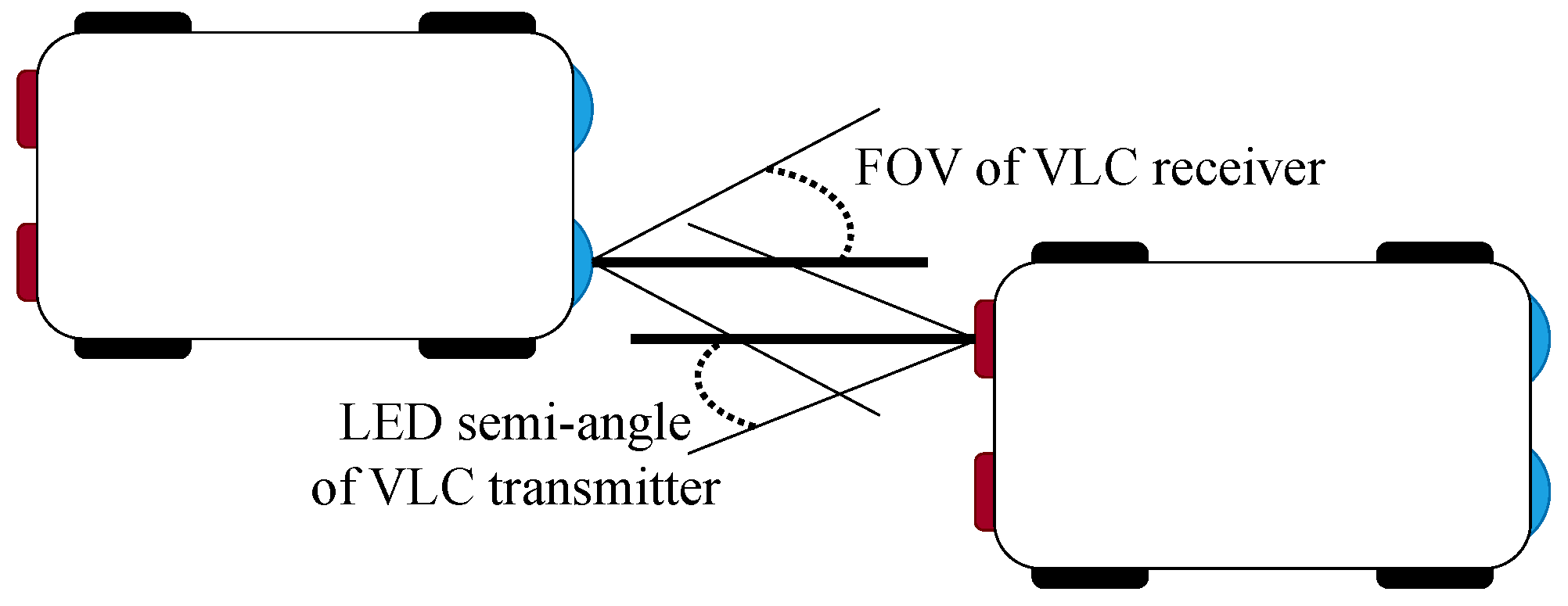
The applications of VANET can be categorized into safety and comfort. The goal of safety applications is to reduce the occurrence of traffic accidents. For example, when a vehicle is expected to collide with another vehicle, the safety message will be immediately transmitted to the driver. Yang et al. proposed an Intersection Collision Warning (ICW) system. The ICW system uses a smart phone to receive safety-related information via on-board GPS receivers. Then, this information is periodically exchanged to compute the probability of collision [22].

Comfort applications aim at improving the comfort of drivers and passengers. For example, drivers can obtain the weather condition or the location of the nearest attraction through VANET applications. Passengers can use VANET to play online games, watch on-demand videos, or send messages [23]. Keshavarzi et al. proposed a method to obtain real-time urban traffic information by combining traditional networks and VANET [3].

2.2. VLC

VLC has received increasing attention in recent years because the current RF spectrum is not enough to accommodate ever-increasing traffic. Moreover, VLC can bring better security, a higher data rate, and lower deployment costs [24]. Generally, the scenarios of applying VLC can be divided into indoor and outdoor. We briefly review related VLC research for indoor and outdoor scenarios.

The research on indoor VLC mainly focuses on accurate positioning. Accurate indoor positioning can provide indoor navigation for users in large shopping centers, airports, or hospitals. However, due to GPS errors usually being as high as tens of centimeters to several meters, it is difficult to achieve accurate indoor positioning. Gradually, some researchers have used VLC for indoor positioning, where VLC can achieve cm-level accuracy without causing electromagnetic interference [25]. Naz et al. proposed an indoor positioning algorithm based on Phase Difference of Arrival (PDOA) for VLC systems. PDOA uses frequency and phase information for target positioning to achieve more accurate positioning [26].

On the other hand, the electromagnetic radiation caused by RF technology for communication could be harmful to humans. As a result, the deployment of RF technology could be limited in hospitals or airports. Therefore, VLC can be used for communication in these facilities. Ding et al. proposed an indoor communication system for hospitals. The proposed communication system combines power lines and the VLC system to achieve a radiation-free, high-capacity, and positionable communication system [27].

As mentioned above, using RF technology for communication often suffers from interference in high-density environments. VLC has interference-free characteristics that make it suitable for a dense area. However, VLC is easily affected by the external environment. Therefore, VLC is usually used to complement RF technology. Chen et al. proposed a distributed non-cooperative topology control for hybrid VLC/RF VANET. The proposed scheme reduces the power consumption and the interference between wireless links by adapting the transmission power of RF and VLC [28]. Ji et al. proposed a multi-hop clustering algorithm for a hybrid VANET architecture with DSRC and VLC. Their algorithm creates clusters by collecting the mobility information of vehicles through VLC receivers [29]. Abualhoul et al. proposed a prediction-based vertical handover mechanism (PVHO). PVHO switches communication between DSRC and VLC based on packet sequence, message length, and the relative orientation of vehicles [30].

VLC can also conduct positioning when vehicles cannot receive GPS signals. Kim et al. proposed a VLC positioning system for VANET. The proposed positioning system senses the LED light source through the camera to obtain the three-dimensional coordinate information of other vehicles [19].

2.3. Clustering Schemes

The high mobility of vehicles may cause vehicles to easily disconnect from each other during data transmission. Moreover, massive connections from vehicles will cause channel congestion and high transmission delay to degrade the performance of real-time applications. Clustering is a viable solution to improve transmission performance. Every cluster will have a CH to manage the data within its cluster and communicate with the infrastructure. Several factors are considered in generating clusters [31], as described below.

2.3.1. Identification and Connectivity

Early typical clustering algorithms include the lowest-ID (LID) algorithm and the highest-connectivity clustering algorithm. The LID algorithm assumes that every node has a unique ID, and the node with the smallest ID will be selected as the CH of the cluster. The highest-connectivity clustering algorithm considers the connection degree of nodes; the node with the highest connection degree will be selected as the CH [32].

2.3.2. Mobility and Signal Quality

The mobility clustering algorithm considers the relative position, relative speed, and moving direction of vehicles for clustering. The above information can be used to calculate the link lifetime (LLT) between a vehicle and its neighbors. The selected CH based on LLT is usually located in the center of vehicles and has a low average speed difference from its CM [33,34]. Ren et al. proposed a mobility-based and stability-based clustering algorithm (MSCA). MSCA considers the distance and position of a vehicle to select the CH, and calculates the LLT between the CH and CM to select a gateway vehicle [35].

In order to improve the communication quality, some researchers have used Received Signal Strength (RSS) and Signal-to-Noise Ratio (SNR) as factors to form clusters [36,37]. Liu et al. proposed a clustering algorithm, which calculates the probability of successful packet transmission between vehicles. Finally, the algorithm combines these factors with the direction and speed of vehicles to select CHs [21].

2.3.3. Size and Intension

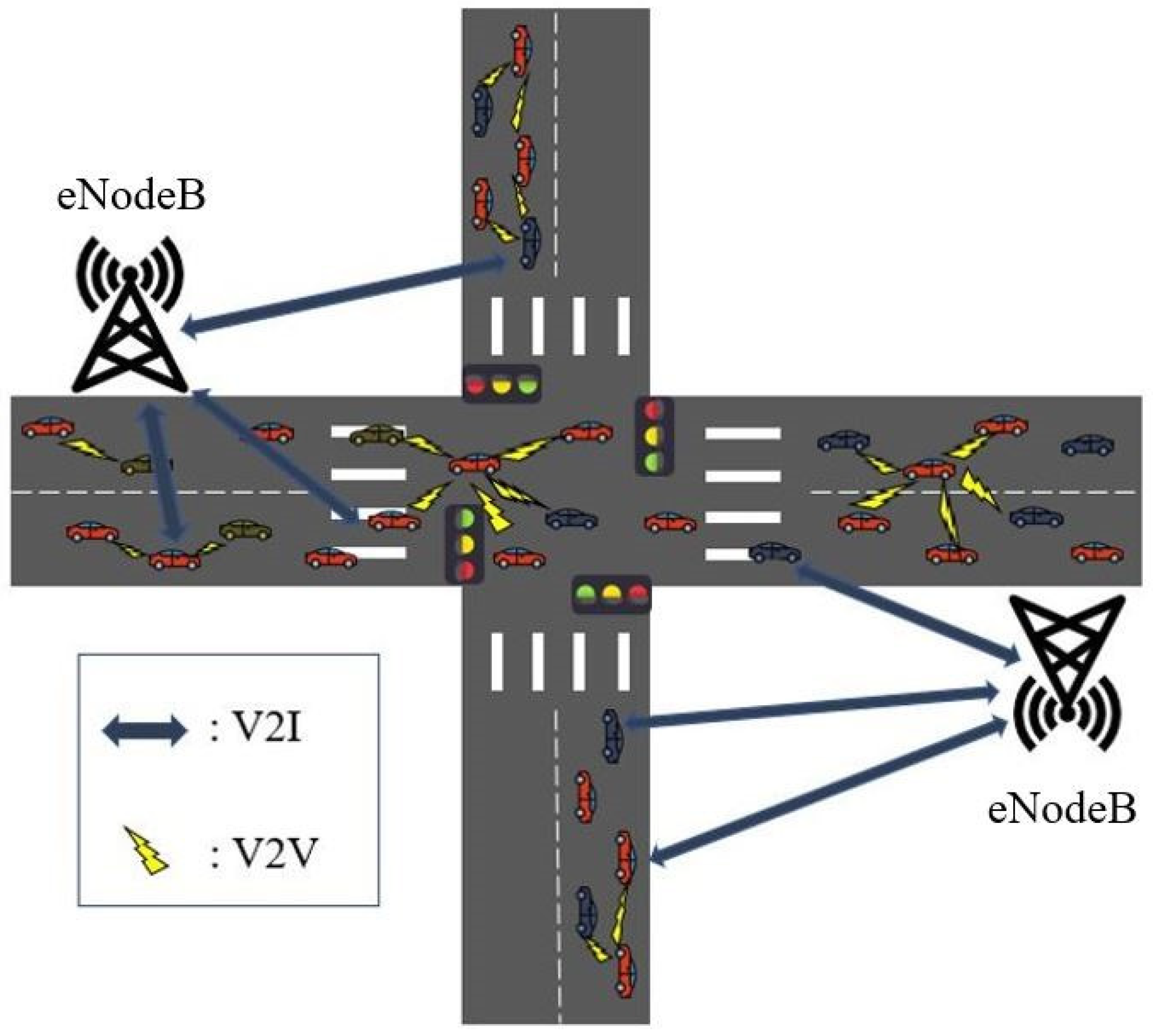
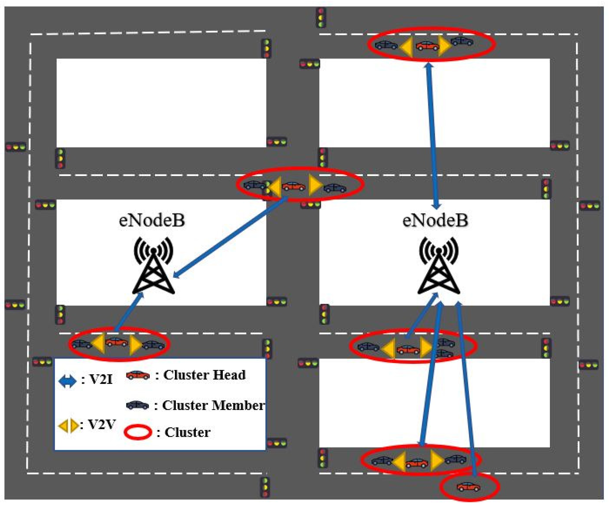
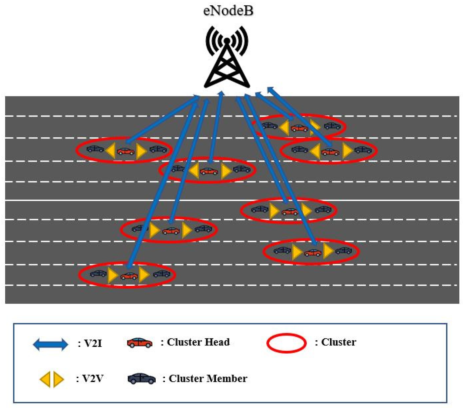
The communication range of vehicles with distinct sizes may be different, and the vehicle itself could be an obstacle. Some researchers consider the vehicle size as one factor to generate clusters. A. Maglaras et al. proposed an Enhanced Spring Clustering (ESC) algorithm, which selects the vehicle with the higher height as the CH in order to cover more vehicles in one cluster [38].

Vehicles may change their directions of movement at junctions to cause disconnection. Some researchers use the driver intension as the factor to form clusters. Tal et al. proposed a user-oriented fuzzy-logic-based clustering scheme. The scheme uses fuzzy logic to combine the mobility of vehicles and the intention of drivers. Thus, vehicles in the same cluster are expected to have similar destinations [39].

3. System Model

In this work, we consider two scenarios in our system model: urban area and highway, as shown in Figure 3 and Figure 4. In both scenarios, there are basestations for connecting vehicles. Vehicles may also communicate with neighboring vehicles through VLC. In our system model, the infrastructure will form clusters based on the number of neighboring vehicles. Vehicles could be a CH or CM. CMs will send their requests to the CH, where the CH is responsible for managing its CMs’ messages and communicating with the infrastructure. We assume that all vehicles are equipped with GPS, an On-Board Unit (OBU), LEDs, and cameras. GPS enables vehicles to obtain current location information. The OBU enables vehicles and the infrastructure to communicate with each other through DSRC and 5G or LTE. LEDs and cameras enable two vehicles with aligned semi-angles and FOVs to communicate with each other. Moreover, VLC relies on the LOS between the transmitter and receiver; thus, any physical obstruction, such as buildings and other vehicles, may block the light signal.

All vehicles use VLC for communication only when it is available. As mentioned above, VLC has the requirement of LOS between the transmitter and receiver. Any block between the transmitter and receiver may result in signal outage, which would interrupt packet forwarding and degrade the performance of applications. In the environments that VLC is unavailable, such as sudden heavy rain or strong sunlight, DSRC is used for communication. In this paper, we focus on the clustering performance based on VLC. Because we consider two-way communication, it is only when the receiver and the transmitter of two vehicles are within the semi-angle of each other that they can establish a communication link. The communication between vehicles and the infrastructure is one-hop. We also assume that a vehicle will transmit its driving route in the current road segment to the infrastructure whenever it enters the road segment. This information will enable the clustering algorithm to estimate the number of neighboring vehicles in a future time period for each vehicle. We also note that the influence of link delay, reliability, and capacity is not considered since these metrics affect the performance of applications, not the performance of vehicle clustering.

4. Problem Statement

We further define the problem of vehicle clustering for VANET based on VLC. We describe some notations for the problem statement first. N represents the set of vehicles for clustering. $H_{i,j}$ represents the hop count between two vehicles, i and j, by using VLC. $D_i$ represents how long the vehicle serves as a CH or CM. $S_{i,j}^{\prime }$ indicates whether the VLC transmitter of vehicle i can be sensed by the receiver of another vehicle j; 1 means yes, 0 means no. $L_{i,j}^{\prime }$ indicates whether the two vehicles, i and j, are connected in the same cluster, where 1 means yes and 0 means no, when two connected vehicles include one cluster head and one cluster member. $C{H}_i^{\prime }$ denotes whether vehicle i is a CH; 1 means yes, 0 means no. $C{M}_i^{\prime }$ represents whether vehicle i is a CM; 1 means yes, 0 means no. All notations are summarized in

Table 1. Notations.

Notation	Description
N	The set of vehicles
$H_{i,j}$	The hop count between $(i,j),\forall i,j\in N$
$D_i$	The duration of i in CH or CM status, $\forall i\in N$
$S_{i,j}^{\prime }$	The binary variable indicates whether j is sensed by $i,\forall i,j\in N$
$L_{i,j}^{\prime }$	The binary variables indicating link between $(i,j),\forall i,j\in N$
$C{H}_i^{\prime }$	The binary variable indicates whether i is CH, $\forall i\in N$
$C{M}_i^{\prime }$	The binary variable indicates whether i is CM, $\forall i\in N$

.

We attempt to generate stable clusters for vehicles, where each vehicle can communicate with the infrastructure through its cluster head. As a result, the number of vehicles communicating with the basestation at the same time can be effectively reduced. By reducing the simultaneous communications between vehicles and the basestation, channel interference can be reduced to improve communication performance. Therefore, the number of clusters (or CHs) should also be minimized. On the other hand, if the connection between vehicles is often disconnected, it will reduce the packet delivery ratio and increase packet delay. Thus, the duration of each CH should be maximized. The objective function is listed in Equation (1) and the constraints are listed in Equations (2)–(5).

$$\begin{array}{cc}\hfill \min & (\sum _{i\in N}C{H}_i^{\prime })and\max \left(D_i\right),whereC{H}_i^{\prime }=1,\forall i\in N\hfill \end{array}$$

(1)

$$\begin{array}{cc}\hfill \mathrm{s}.\mathrm{t}.& C{H}_i^{\prime }+C{M}_i^{\prime }=1,\forall i\in N\hfill \\ & L_{i,j}^{\prime }=1,\mathrm{if}C{H}_i^{\prime },C{M}_j^{\prime },S_{i,j}^{\prime },S_{j,i}^{\prime },H_{i,j}=1\hfill \end{array}$$

(2)

$$\begin{array}{cc}& \forall i,j\in N\hspace{1em}\hspace{1em}\hspace{1em}\hspace{1em}\hspace{1em}\hspace{1em}\hfill \end{array}$$

(3)

$$\begin{array}{cc}& \sum _{i\in N}{L}_{i,j}^{\prime }=\sum _{i\in N}C{M}_i^{\prime },\forall i\in N\hfill \end{array}$$

(4)

$$\begin{array}{cc}& C{H}_i^{\prime },C{M}_i^{\prime },L_{i,j}^{\prime }\in \{0,1\}\hfill \end{array}$$

(5)

Equation (1) shows that our goal is to minimize the number of CHs and maximize their duration. Equation (2) ensures that every vehicle will only have one state, either CH or CM. A vehicle can be a CH and a CM at the same time. Equation (3) identifies the conditions for when two vehicles have a connecting link. Equation (4) requires that every CM only selects one CH for connection. Equation (5) shows the binary property. In previous research, the CH optimization problem has been shown as an NP-hard problem [40].

5. Proposed Algorithm

To accommodate vehicles whose positions change rapidly, we use a greedy clustering method to reduce the number of CHs while maintaining their duration. We consider two factors to generate clusters: the number of neighbors and the directions of vehicles. Selecting a vehicle with a larger number of neighbors as the CH could allow more vehicles to join the cluster. Therefore, the total number of CHs can be effectively reduced. If the moving direction between the CH and CMs are different, the CH and its CMs may be disconnected immediately, affecting the number of neighboring vehicles as well as the CH duration.

5.1. Neighbor List Creation

Since we use the number of neighbors as the first factors for cluster generation, the first step of our scheme creates a neighbor list (N) for every vehicle. Vehicle i uses its receiver to sense the light waves within its semi-angle from other vehicles j. There are two cases to determine whether the received light wave is from its neighbor. In the first case, if the current position of vehicle i is in a road segment, vehicle i will only add vehicles that move in the same direction to $N_i$. This is because the vehicles of different driving directions will disconnect from each other soon. In the second case, if the current position of vehicle i is in a junction, vehicle i will directly add all sensed vehicles to $N_i$. Moreover, in our scenario, a vehicle will only give its driving route in the current road segment to the infrastructure when it enters a road segment. The complete process of creating a neighbor list is listed in Algorithm 1.

5.2. CH Selection

After all vehicles have created their neighbor lists, vehicles will transmit the information to the infrastructure for selecting CHs. For vehicles whose current status is not a CH or a CM, the one with a higher number of neighbors ($\left|N\right|$) is assigned as the CH. We note that every vehicle can only have one state (CH or CM) at the same time. If vehicle i has been selected as the CH or CM and also appears in the neighbor lists of other vehicles, the infrastructure will remove vehicle i from other neighbor lists to avoid other vehicles becoming a CH or CM at the same time. The complete process of selecting CHs is listed in Algorithm 2.

Algorithm 1 Neighbor List Creation

1: for every vehicle i do 2:    for every vehicle j do 3:      if $i\ne j$ then 4:         if j is on a junction then 5:           if (the light wave of j is within the semi-angle of i’s receiver) and (the light wave of i is within the semi-angle of j’s receiver) then 6:              $N_i⟵j$ 7:           end if 8:         else if i is on a road segment then 9:           if (j is moving in same direction with i) and (the light wave of j is within the semi-angle of i’s receiver) and (the light wave of i is within the semi-angle of j’s receiver) then 10:              $N_i⟵j$ 11:           end if 12:         end if 13:      end if 14:    end for 15: end for

Algorithm 2 CH Selection

1: while there is vehicle that are not selected as CH or CM do 2:    for every vehicle i with $|N_i|==0$ do 3:      CH $⟵i$ 4:    end for 5:    CH ⟵ The vehicle i with the highest $\left|N\right|$ in vehicles that are not CH or CM 6:    for every vehicle j in $N_i$ do 7:      CM $⟵j$ 8:      for every vehicle k that are not selected as CH or CM do 9:         for every vehicle m in $N_k$ do 10:           if ($m==i$) or ($m==j$) then 11:              remove m from $N_k$ 12:           end if 13:         end for 14:      end for 15:    end for 16: end while

5.3. $|N_f|$ Construction

Although CHs can be calculated based on the previous algorithm, the high mobility of vehicles and the non-penetrating characteristic of VLC may reduce the duration of CHs. Therefore, we set a timespan ($T_{\left(e\right)}$) with a repeated countdown. Then, we use the driving routes of vehicles to estimate the number of neighbors per vehicle ($|N_f|$) within the future $T_{\left(e\right)}$ time. The driving routes of vehicles are calculated based on the movements of vehicles as they enter a road segment. The movement information of a vehicle includes speed, direction, and its current position. We use the calculated $|N_f|$ instead of $\left|N\right|$ for CH selection. The goal is to prolong the CH duration. The calculation of $|N_f|$ is related to when the vehicle appears on the network, as shown in Equation (6). The equation shows that if a vehicle joins the network at the $k_{th}$ second, the time for estimating $|N_f|$ will start from the $k_{th}$ second to the end of $T_{\left(e\right)}$. For the sake of fair comparisons, we divide the sum of $\left|N\right|$ for each vehicle during the period by the time that the vehicle appears in $T_{\left(e\right)}$.

$$\left|N_f\right|=\begin{array}{c}\frac{{\sum }_k^{T_{\left(e\right)}}\left|N_i^k\right|}{t},\hfill \end{array}$$

(6)

where k is the second that the vehicle i enters the road segment and t is the number of seconds in $T_{\left(e\right)}$ that vehicle appears in the road segment.

Initially, the infrastructure selects a value of $T_{\left(e\right)}$ and calculates N for every vehicle. Then, the infrastructure calculates $|N_f|$ for every vehicle before $T_{\left(e\right)}$ starts. Finally, the infrastructure uses $|N_f|$ instead of $\left|N\right|$ to select CHs. If a new vehicle joins the network before $T_{\left(e\right)}$ starts, the infrastructure first calculates its $|N_f|$ for this vehicle. Then, it checks whether the appearance of this vehicle has affected the $|N_f|$ values of the existing vehicles. If the answer is yes, the infrastructure updates the $|N_f|$ values for the affected vehicles. Otherwise, the $|N_f|$ of this vehicle remains unchanged. The complete process of $|N_f|$ construction is listed in Algorithm 3.

Algorithm 3 $|N_f|$ Construction

1: Initialize: Infrastructure set up $T_{\left(e\right)}$ to evaluate $|N_f|$ of every vehicle 2: for every second in $T_{\left(e\right)}$ do 3:    if (vehicle i enters the road segment) or (the driving route of vehicle i is changed)    then 4:      i transmit its new driving route to infrastructure 5:    end if 6:    if $T_{\left(e\right)}$ has not counted down then 7:      for every vehicle i do 8:         Infrastructure calculates $|N_f^i|$ by using driving route of vehicle and Algorithm 1 9:       end for 10:    else 11:      if there are new vehicles j joining the network then 12:         Infrastructure calculates $|N_f^j|$ by using driving route of vehicle and Algorithm 1 13:         for every vehicle i do 14:           Infrastructure inspect whether j affects $|N_f^i|$ 15:           if $|N_f^i|$ is affected by j then 16:              Infrastructure recalculate $|N_f^i|$ 17:           else 18:              $|N_f^i|$ remains unchanged 19:           end if 20:         end for 21:      end if 22:    end if 23: end for

6. Simulation Results

In this section, we evaluate the performance of the proposed clustering algorithm based on the number of neighbors (CBN) and the enhanced version based on the estimated number of neighbors in the time period (E-CBN). CBN selects the vehicles with higher $\left|N\right|$ values as CHs, and E-CBN selects the CH based on the value of $|N_f|$. We also relate our algorithms with the following algorithms for performance comparison. The first is the clustering algorithm based on LLT (CBL). The second is the LID clustering algorithm. CBL chooses the vehicle with higher LLT as the CH, and LID selects CHs based on their identifiers. All cluster algorithms were implemented by using Python. The vehicular trace file was generated by Simulation of Urban Mobility (SUMO) [41].

6.1. Parameter Settings and Performance Metrics

Two scenarios are considered in our simulations, urban area and highway, as shown in Figure 3 and Figure 4. The map size of the urban area is $600\ast 700$ m${}^2$. There are three lanes in each direction of each road segment and eight junctions with traffic signs in the urban area, where the speed limit is 40 km per hour [42]. The length of the highway scenario is 5 km. There are five lanes in each direction, and the speed limit is 80 km per hour [43]. The total number of vehicles in the urban area and highway is 500. The initial position of every vehicle and its driving route are random. The semi-angle of the transmitter is 10 [18]. The transmission range of each vehicle is 100 m [12]. The total simulation time is 80 s. We set different values of $T_{\left(e\right)}$ to evaluate the influence of the estimated positions of vehicles. Because we need to calculate the data transmission rate of every vehicle as a performance metric in our simulation, we set the following parameters for the calculation: The transmission range of the roadside unit (RSU) is 680 m based on the coverage of 5G base stations [44]. Then, the number of RSUs to cover each scenario is calculated, where the number of RSUs in the highway is seven and that in the urban area is two. Every RSU has five channels for vehicles to join randomly [45]. The channel bandwidth is 100 MHz [44]. The transmission power of a vehicle is 200 mWatts [46]. The channel noise is ${10}^{-10}$ mWatts [45]. The path loss factor is 4 [45]. We calculate the data rate of each CH first, and the CMs of a CH share the available bandwidth. The data rate of CHs can be calculated by using Equation (7). The parameters used in our simulation are summarized in

Table 2. Simulation parameters.

Parameters	Urban Area	Highway
Map Size	600 m×700 m	5000 m × 100 m
Maximum Speed	40 km/h [42]	80 km/h [43]
Lanes (each direction)	3	5
Total Number of Vehicles	500	500
Semi-angle	${10}^{\circ }$ [18]	${10}^{\circ }$ [18]
Transmission Range of Vehicle	100 m [12]	100 m [12]
Simulation Time	80 s	80 s
$T_{\left(e\right)}$	20 s	10 s
Transmission Range of RSUs	680 m [44]	680 m [44]
Total Number of RSUs	2	7
Number of Channels	5 [45]	5 [45]
Channel Bandwidth	100 MHz [44]	100 MHz [44]
Transmission Power of Vehicle	200 mWatts [46]	200 mWatts [46]
Channel Noise	10${}^{-10}$ mWatts [45]	10${}^{-10}$ mWatts [45]
Path Loss Factor	4 [45]	4 [45]

.

$$r_i=Wlo{g}_2\left(1+\frac{p_i{g}_i}{\omega +{\sum }_{j\ne i,j\in C}{p}_j{g}_j}\right),\forall i,j\in \mathrm{CH},$$

(7)

where W is the channel bandwidth. p is the transmission power of the vehicle. g is the channel gain between vehicle and infrastructure. C is the set of CHs that stay in the same channel. $\omega$ is the channel noise. The channel gain g is calculated by using Equation (8).

$$g_i=d_i^{\alpha },$$

(8)

where d is the distance between the CH and the infrastructure and $\alpha$ is the path loss factor.

We evaluate the performance of different clustering algorithms based on the following performance metrics:

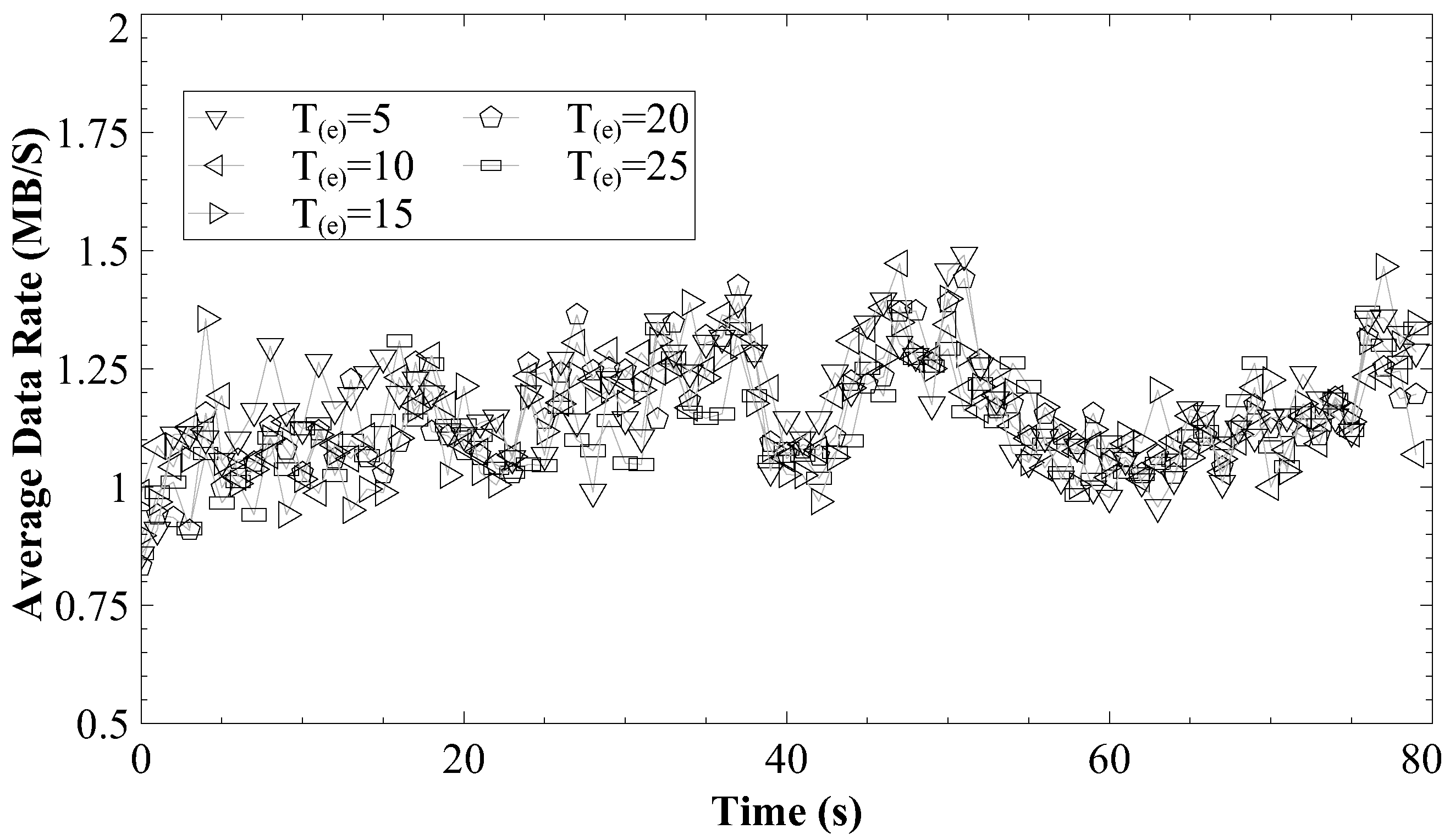
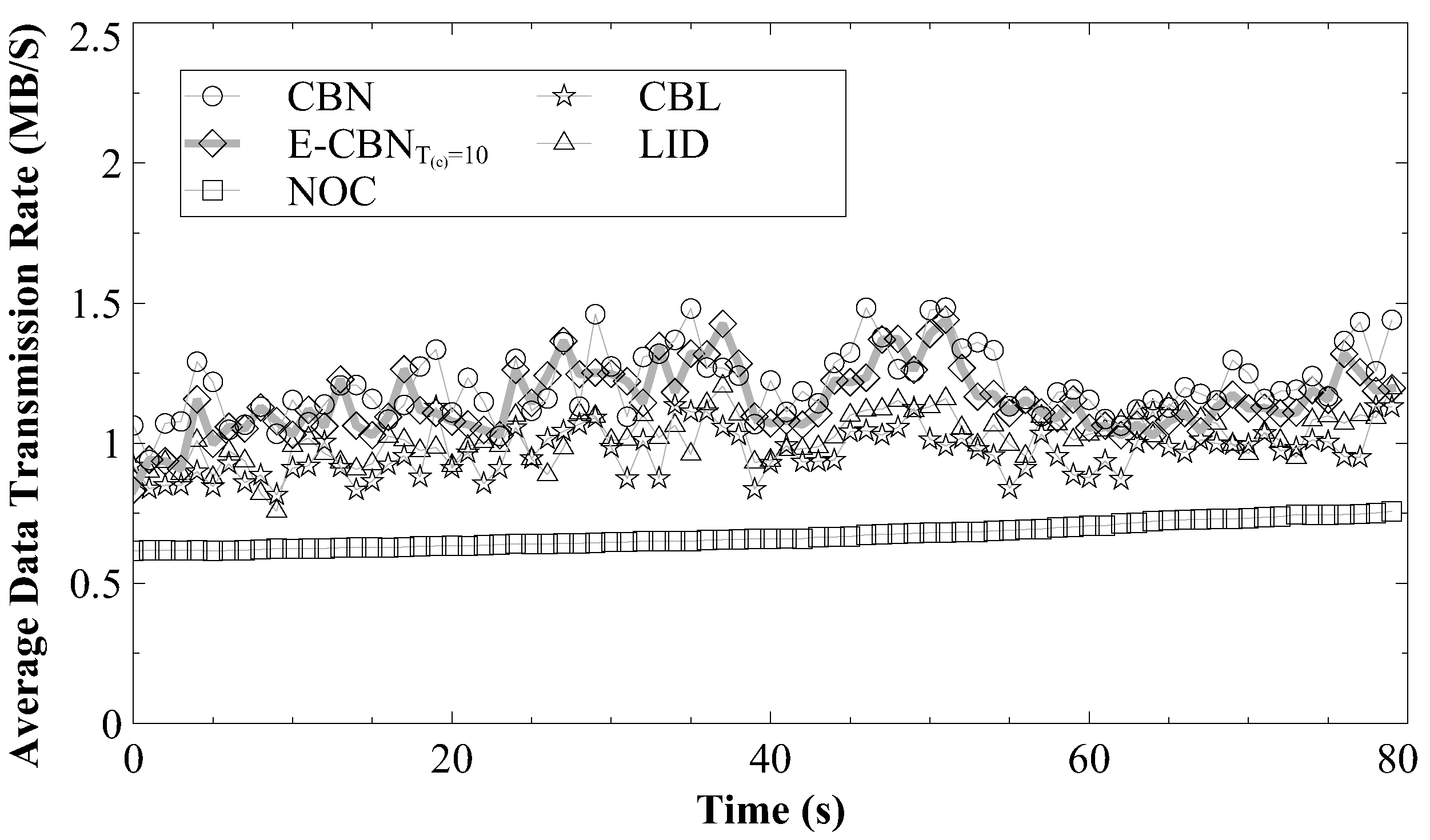
• The average data rate: the average data rate of all vehicles for uploading.
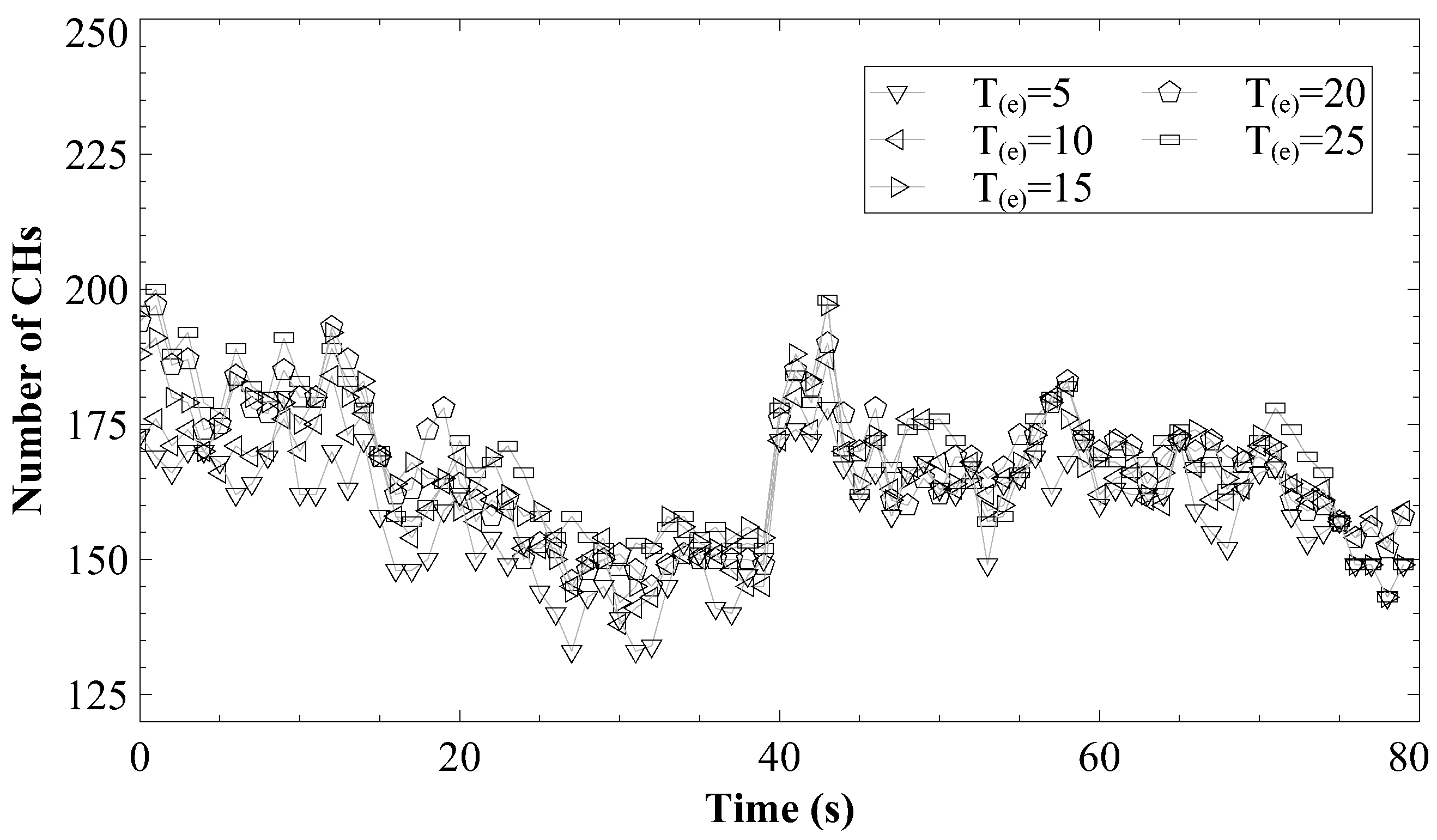
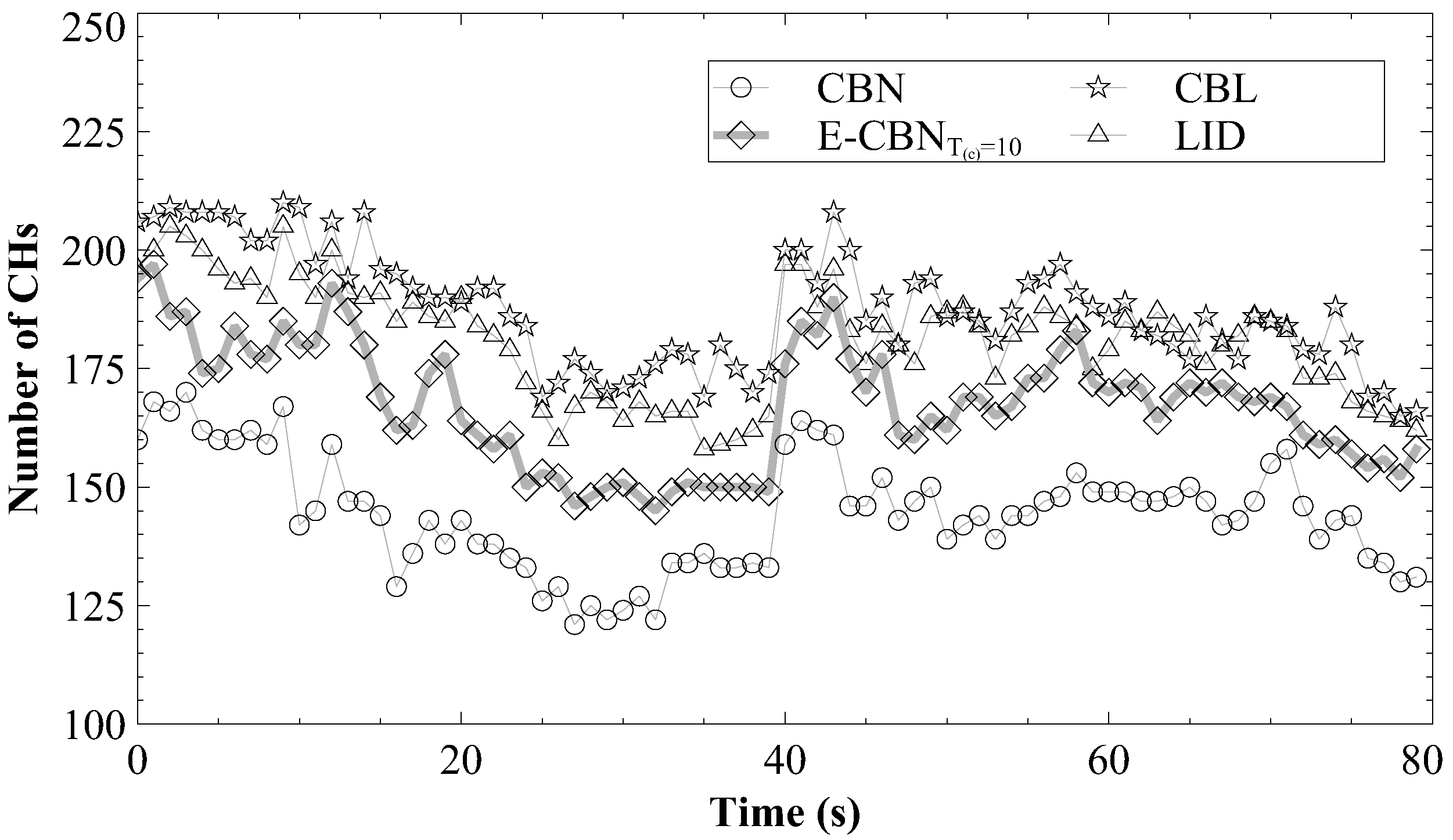
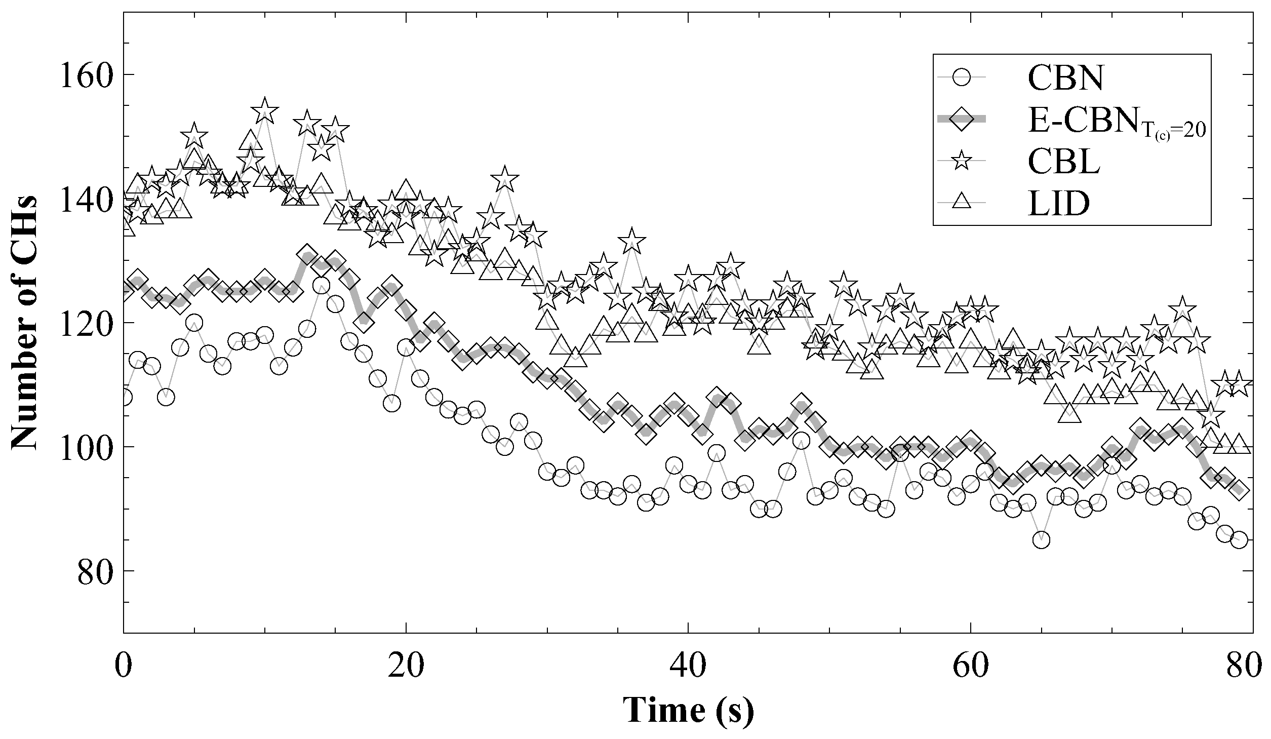
• The number of CHs: The number of CHs selected by a clustering algorithm. The lower number of CHs also represents that the possibility of numerous vehicles uploading data to the infrastructure simultaneously can be reduced.
• The number of CH changes: The number of times that vehicles change their states from CH to CM. A lower number of CH changes can reduce the communication overhead for the original CMs.
• The number of CM changes: The number of times that vehicles change their states from CM to CH. Since a CM changing its state to CH will notify its original CH and new CMs, a lower number of CM changes can reduce the communication overhead. A new CH will also contact the RSU to announce its presence.
• The CH duration: The duration of a vehicle serving as a CH. A higher CH duration implies a lower number of control messages.

6.2. Results Analysis

First, we will analyze the effect of different $T_{\left(e\right)}$ on E-CBN in order to select the most suitable $T_{\left(e\right)}$ value for our algorithm. Because there are similar trends in the highway and urban area, we only present the analysis results of urban area here. Figure 5 and Figure 6 show the average data rate and the number of CHs for different values of $T_{\left(e\right)}$. The results show that as the value of $T_{\left(e\right)}$ increases, the average data rate decreases but the number of CHs increases. This is because when $T_{\left(e\right)}$ is longer, a vehicle with the most neighbors currently may not be selected as a CH owing to estimated vehicle movements. As a result, more vehicles are selected as CHs. Since there are more CHs for larger $T_{\left(e\right)}$ values, the average number of CMs per CH is reduced as well.

Table 3. The average CH duration, the number of CH and CM changes for different $T_{\left(e\right)}$ in urban area.

Metrics	${\mathit{T}}_{\left(\mathit{e}\right)}=5$	${\mathit{T}}_{\left(\mathit{e}\right)}=10$	${\mathit{T}}_{\left(\mathit{e}\right)}=15$	${\mathit{T}}_{\left(\mathit{e}\right)}=20$	${\mathit{T}}_{\left(\mathit{e}\right)}=25$
Average CH duration (s)	$5.4$	$7.0$	$7.7$	$7.7$	$7.9$
The number of CH changes	2729	2219	2142	2082	2108
The number of CM changes	2878	2378	2291	2240	2257

lists the average CH duration and the number of CH and CM changes for different $T_{\left(e\right)}$ values. Although a larger $T_{\left(e\right)}$ value would result in more CHs, it also prolongs the average CH duration and decreases the number of CH and CM changes. This is because a larger $T_{\left(e\right)}$ value can reduce the occurrences of selecting a vehicle with a higher number of neighbors only for a short time period. Therefore, vehicles can maintain their states consistently with longer CH duration.

It can be seen from this simulation that a longer $T_{\left(e\right)}$ value can improve the stability of vehicle states but also result in more CHs. In order to keep vehicle states stable without incurring too many CHs, we set $T_{\left(e\right)}$ to 10 s and 20 s in the urban area and highway, respectively.

Next, we show the simulation results for different clustering algorithms in the urban area. Figure 7 and Figure 8 show the average data rate and the number of CHs for different clustering algorithms per second. The data rate without generating any cluster is also included for comparison (NOC). Obviously, the average data rate of NOC is the lowest because all vehicles compete for limited bandwidth. CBL and LID have the second-worst average data rate and the highest number of CHs because CBL only considers the LLT for CH selection and LID only selects the vehicle with the smallest ID as the CH. Both algorithms ignore the connection degree of vehicles. As a result, their CHs have lower numbers of CMs than the other algorithms. As compared with E-CBN, the average data rate of CBN is improved by $5\%$ on average. The total number of CHs is also reduced by $14\%$. This is because CBN always selects the vehicles with the most neighbors to minimize the number of CHs. In contrast, the CHs selected by E-CBN may not be the best at the moment, but these CHs can usually last longer by considering vehicle movements.

Table 4. Performance comparisons for different clustering algorithm in urban area.

Metrics	CBN	E-CBN${}_{{\mathit{T}}_{\left(\mathit{e}\right)}=10}$	CBL	LID
Average CH duration (s)	$3.7$	$7.7$	$3.1$	$10.9$
The number of CH changes	3440	2082	5375	1811
The number of CM changes	3571	2240	5541	1973

shows the average CH duration and the numbers of CH and CM changes for different clustering algorithms in the urban area. CBL has a short CH duration and leads to the most CH and CM changes. LLT is used to indicate the time period that two vehicles could communicate with each other, but the VLC between two nearby vehicles could still be blocked by other vehicles, causing frequent disconnection. Although the number of CHs in E-CBN is $14\%$ more than CBN, the average CH duration and the number of CH and CM changes of E-CBN are improved by $52\%$ and $39\%$, or $37\%$ as compared to CBN because $|N_f|$ is updated only when a new vehicle joins the network or the next $T_{\left(e\right)}$ time frame starts. As a result, the vehicle states can be smoothly updated by E-CBN. LID has the best CH duration and number of CH and CM changes since vehicle IDs do not change.

Next, we show the simulation results of different clustering algorithms in the highway. Figure 9 and Figure 10 show the average data rate and the number of CHs in different clustering algorithms. As compared to the urban area, the average data rate is increased due to the additional number of RSUs in the highway. The difference in the total number of CHs among all clustering algorithms is also reduced because vehicles are scattered in the larger map of the highway. Similarly, NOC has the worst average data rate. CBL and LID have the second-worst average data transmission rate and number of CHs because of their approaches to selecting CHs. As compared with E-CBN, the average data rate of CBN is improved by $11\%$ on average. The total number of CHs is also reduced by $9\%$.

Table 5. Performance comparisons for different clustering algorithms in the highway.

Metrics	CBN	E-CBN${}_{{\mathit{T}}_{\left(\mathit{e}\right)}=20}$	CBL	LID
Average CH duration (s)	$3.9$	$7.8$	$2.8$	$12.6$
The number of CH changes	2352	1286	4498	1170
The number of CM changes	2437	1379	4608	1270

shows the average CH duration and the number of CH and CM changes for different clustering algorithms in the highway. As compared to the results in the urban area, the performances of all clustering algorithms are significantly improved in the highway because all vehicles can only move straight forward in the highway. CBL still has the shortest CH duration and the highest number of CH and CM changes owing to the LOS characteristic of VLC. LID has the best CH duration and number of CH and CM changes in the highway. Because all vehicles move straight forward in the highway, the vehicle status remains unchanged unless a CH connects to another CH with a smaller ID. E-CBN can improve the CH duration of CBN by 100%. It also greatly reduces the number of CH and CM changes. The results suggest that the proposed clustering algorithm based on vehicle movements can effectively generate stable clusters of vehicles.

Next, we analyze the performance differences for different values of semi-angle, ${10}^{\circ }$, ${50}^{\circ }$, and ${90}^{\circ }$. A wider semi-angle can relax the LOS requirements to enable communication even when vehicles are not perfectly aligned. As a result, when the semi-angle increases, each vehicle can identify more vehicles to result in larger clusters.

Table 6. The average data rate of CHs for clustering algorithms with different values of semi-angle in the urban area.

Semi-Angle	CBN	E-CBN${}_{{\mathit{T}}_{\left(\mathit{e}\right)}=10}$	CBL	LID
${10}^{\circ }$	$1.21$	$1.15$	$0.97$	$1.02$
${50}^{\circ }$	$1.61$	$1.5$	$1.18$	$1.22$
${90}^{\circ }$	$1.74$	$1.57$	$1.26$	$1.26$

and

Table 7. The total number of CHs for clustering algorithms with different values of semi-angle in the urban area.

Semi-Angle	CBN	E-CBN${}_{{\mathit{T}}_{\left(\mathit{e}\right)}=10}$	CBL	LID
${10}^{\circ }$	11,547	13,385	15,017	14,486
${50}^{\circ }$	8480	9776	11,492	11,162
${90}^{\circ }$	7932	9171	10,942	10,624

show that the total number of CHs can be decreased with a wider semi-angle. Moreover, the data rate of CHs is increased with fewer CHs. Among these clustering algorithms, CBN has the best performance and E-CBN has the second-best performance.

Table 8. The average CH duration for different clustering algorithms with different semi-angle in the urban area.

Semi-Angle	CBN	E-CBN${}_{{\mathit{T}}_{\left(\mathit{e}\right)}=10}$	CBL	LID
${10}^{\circ }$	$3.7$	$7.7$	$3.1$	$10.9$
${50}^{\circ }$	3	$6.1$	$2.3$	$7.7$
${90}^{\circ }$	$2.7$	$5.3$	$2.1$	$7.3$

shows the CH duration of different clustering algorithms for different values of semi-angle. As the semi-angle increases, the CH duration is decreased since a wider semi-angle may result in more connected vehicles and larger clusters. As a result, more vehicles could be candidates of the CHs to shorten the CH duration. The results suggest that a wider semi-angle of VLC may degrade the stability of vehicle clusters.

7. Conclusions

In this paper, we propose a clustering algorithm for VANET, where the communication between vehicles is based on VLC. Our algorithm generates vehicle clusters by estimating the number of neighbors per vehicle for a forthcoming time period. The operations of the proposed algorithm include the estimation of vehicle movements and the CH selection. The estimation of vehicle movements considers the current positions, speed, and directions of vehicles to calculate their positions after a predefined time frame. With the estimated positions of vehicles, the algorithm of CH selection can select vehicles with consistent connectivity as CHs to improve the stability of clusters. We conducted a comprehensive simulation to evaluate the performance of our algorithm. Our simulation results show that the proposed algorithm can control the number of CHs and prolong the lifetime of CHs. The number of CHs can be reduced by more than 7% and 11% for urban and highway scenarios, respectively. The lifetime of each CH is also extended twice as compared to the previous algorithms based on the connectivity among vehicles. Moreover, the transmission data rate is improved by 12% to promote the effectiveness of vehicular applications. The performance improvement can be further raised for cases with large semi-angles of VLC, where the transmission data rate of our algorithm outperforms the previous algorithms by more than 20%. As a result, our algorithm can effectively improve the stability of clusters in VANET to achieve reliable and efficient communication for vehicles by using VLC.

References

1. Eze, E.C.; Zhang, S.; Liu, E. Vehicular Ad Hoc Networks (VANETs): Current State, Challenges, Potentials and Way Forward. In Proceedings of the 2014 20th International Conference on Automation and Computing, Cranfield, UK, 12–13 September 2014. [Google Scholar]
2. Ucar, S.; Ergen, S.C.; Ozkasap, O. Multihop-Cluster-Based IEEE 802.11p and LTE Hybrid Architecture for VANET Safety Message Dissemination. IEEE Trans. Veh. Technol. 2016, 65, 2621–2636. [Google Scholar] [CrossRef] [Green Version]
3. Khosroshahi, A.H.; Keshavarzi, P.; KoozehKanani, Z.D.; Sobhi, J. Acquiring Real Time Traffic Information Using VANET and Dynamic Route Guidance. In Proceedings of the 2011 IEEE 2nd International Conference on Computing, Control and Industrial Engineering, Wuhan, China, 20–21 August 2011. [Google Scholar]
4. Xu, C.; Quan, W.; Vasilakos, A.V.; Zhang, H.; Muntean, G.M. Information-centric cost-efficient optimization for multimedia content delivery in mobile vehicular networks. Comput. Commun. 2017, 99, 93–106. [Google Scholar] [CrossRef]
5. Ansari, S.; Boutaleb, T.; Sinanovic, S.; Gamio, C.; Krikidis, I. MHAV: Multitier Heterogeneous Adaptive Vehicular Network with LTE and DSRC. ICT Express 2017, 3, 199–203. [Google Scholar] [CrossRef]
6. Wu, X.; Subramanian, S.; Guha, R.; White, R.G.; Li, J.; Lu, K.W.; Bucceri, A.; Zhang, T. Vehicular Communications Using DSRC: Challenges, Enhancements, and Evolution. IEEE J. Sel. Areas Commun. 2013, 31, 399–408. [Google Scholar]
7. Shen, W.H.; Tsai, H.M. Testing Vehicle-to-Vehicle Visible Light Communications in Real-World Driving Scenarios. In Proceedings of the 2017 IEEE Vehicular Networking Conference (VNC), Torino, Italy, 27–29 November 2017. [Google Scholar]
8. Schettler, M.; Memedi, A.; Dressler, F. Deeply Integrating Visible Light and Radio Communication for Ultra-High Reliable Platooning. In Proceedings of the 2019 15th Annual Conference on Wireless On-demand Network Systems and Services (WONS), Wengen, Switzerland, 22–24 January 2019. [Google Scholar]
9. Junior, W.L.; Costa, J.; Rosário, D.; Cerqueira, E.; Villas, L.A. A Comparative Analysis of DSRC and VLC for Video Dissemination in Platoon of Vehicles. In Proceedings of the 2018 IEEE 10th Latin-American Conference on Communications (LATINCOM), Jalisco, Mexico, 14–16 November 2018. [Google Scholar]
10. Ucar, S.; Ergen, S.C.; Ozkasap, O. Security Vulnerabilities of IEEE 802.11p and Visible Light Communication Based Platoon. In Proceedings of the 2016 IEEE Vehicular Networking Conference (VNC), Columbus, OH, USA, 8–10 December 2016. [Google Scholar]
11. Masini, B.M.; Bazzi, A.; Zanella, A. Vehicular Visible Light Networks with Full Duplex Communications. In Proceedings of the 2017 5th IEEE International Conference on Models and Technologies for Intelligent Transportation Systems (MT-ITS), Napoli, Italy, 26–28 June 2017. [Google Scholar]
12. Uysal, M.; Ghassemlooy, Z.; Bekkali, A.; Kadri, A.; Menouar, H. Visible Light Communication for Vehicular Networking: Performance Study of a V2V System Using a Measured Headlamp Beam Pattern Model. IEEE Veh. Technol. Mag. 2015, 10, 45–53. [Google Scholar] [CrossRef]
13. Do, T.H.; Yoo, M. A Multi-Feature LED Bit Detection Algorithm in Vehicular Optical Camera Communication. IEEE Access 2019, 7, 95797–95811. [Google Scholar] [CrossRef]
14. Islam, A.; Musavian, L.; Thomos, N. Performance Analysis of Vehicular Optical Camera Communications: Roadmap to uRLLC. In Proceedings of the 2019 IEEE Global Communications Conference (GLOBECOM), Big Island, HI, USA, 9–13 December 2019. [Google Scholar]
15. Takai, I.; Harada, T.; Andoh, M.; Yasutomi, K.; Kagawa, K.; Kawahito, S. Optical Vehicle-to-Vehicle Communication System Using LED Transmitter and Camera Receiver. IEEE Photonics J. 2014, 6, 7902513. [Google Scholar] [CrossRef]
16. Khan, L.U. Visible light communication: Applications, architecture, standardization and research challenges. Digit. Commun. Netw. 2017, 3, 78–88. [Google Scholar] [CrossRef] [Green Version]
17. Eso, E.; Burton, A.; Hassan, N.B.; Abadi, M.M.; Ghassemlooy, Z.; Zvanovec, S. Experimental Investigation of the Effects of Fog on Optical Camera-based VLC for a Vehicular Environment. In Proceedings of the 2019 15th International Conference on Telecommunications (ConTEL), Graz, Austria, 3–5 July 2019. [Google Scholar]
18. Shaaban, R.; Faruque, S. Cyber security vulnerabilities for outdoor vehicular visible light communication in secure platoon network: Review, power distribution, and signal to noise ratio analysis. Phys. Commun. 2020, 40, 101094. [Google Scholar] [CrossRef]
19. Kim, B.W.; Jung, S.Y. Vehicle Positioning Scheme using V2V and V2I Visible Light Communications. In Proceedings of the 2016 IEEE 83rd Vehicular Technology Conference (VTC Spring), Nanjing, China, 15–18 May 2016. [Google Scholar]
20. Bali, R.S.; Kumar, N.; Rodrigues, J.J. Clustering in vehicular ad hoc networks: Taxonomy, challenges and solutions. Veh. Commun. 2014, 1, 134–152. [Google Scholar] [CrossRef]
21. Liu, L.; Chen, C.; Qiu, T.; Zhang, M.; Li, S.; Zhou, B. A data dissemination scheme based on clustering and probabilistic broadcasting in VANETs. Veh. Commun. 2018, 13, 78–88. [Google Scholar] [CrossRef]
22. Yang, J.; Wang, J.; Liu, B. An Intersection Collision Warning System using Wi-Fi Smartphones in VANET. In Proceedings of the 2011 IEEE Global Telecommunications Conference—GLOBECOM 2011, Houston, TX, USA, 5–9 December 2011. [Google Scholar]
23. Al-Sultan, S.; Al-Doori, M.M.; Al-Bayatti, A.H.; Zedan, H. A comprehensive survey on vehicular Ad Hoc network. J. Netw. Comput. Appl. 2014, 37, 380–392. [Google Scholar] [CrossRef]
24. Pathak, P.H.; Feng, X.; Hu, P.; Mohapatra, P. Visible Light Communication, Networking, and Sensing: A Survey, Potential and Challenges. IEEE Commun. Surv. Tutor. 2015, 17, 2047–2077. [Google Scholar] [CrossRef]
25. Guan, W.; Wu, Y.; Wen, S.; Chen, H.; Yang, C.; Chen, Y.; Zhang, Z. A novel three-dimensional indoor positioning algorithm design based on visible light communication. Opt. Commun. 2017, 392, 282–293. [Google Scholar] [CrossRef]
26. Naz, A.; Asif, H.M.; Umer, T.; Kim, B.S. PDOA Based Indoor Positioning Using Visible Light Communication. IEEE Access 2018, 6, 7557–7564. [Google Scholar] [CrossRef]
27. Ding, W.; Yang, F.; Yang, H.; Wang, J.; Wang, X. A hybrid power line and visible light communication system for indoor hospital applications. Comput. Ind. 2015, 68, 170–178. [Google Scholar] [CrossRef]
28. Chen, J.; Wang, Z. Topology Control in Hybrid VLC/RF Vehicular Ad-Hoc Network. IEEE Trans. Wirel. Commun. 2020, 19, 1965–1976. [Google Scholar] [CrossRef]
29. Ji, Y.; Yue, P.; Cui, Z. VANET 2.0: Integrating Visible Light with Radio Frequency Communications for Safety Applications. In Proceedings of the ICCCS 2016: Cloud Computing and Security, Nanjing, China, 29–31 July 2016; pp. 105–116. [Google Scholar]
30. Abualhoul, M.; Al-Bado, M.; Shagdar, O.; Nashashibi, F. A Proposal for VLC-Assisting IEEE802.11p Communication for Vehicular Environment Using a Prediction-based Handover. In Proceedings of the ITSC 2018—21st IEEE International Conference on Intelligent Transportation Systems, Maui, HI, USA, 4–7 November 2018. [Google Scholar]
31. Cooper, C.; Franklin, D.; Ros, M.; Safaei, F.; Abolhasan, M. A Comparative Survey of VANET Clustering Techniques. IEEE Commun. Surv. Tutor. 2017, 19, 657–681. [Google Scholar] [CrossRef]
32. Gerla, M.; Tsai, J.T.C. Multicluster, mobile, multimedia radio network. Wirel. Netw. 1995, 1, 255–265. [Google Scholar] [CrossRef]
33. Ren, M.; Zhang, J.; Khoukhi, L.; Labiod, H.; Vèque, V. A Unified Framework of Clustering Approach in Vehicular Ad Hoc Networks. IEEE Trans. Intell. Transp. Syst. 2018, 19, 1401–1414. [Google Scholar] [CrossRef]
34. Rossi, G.V.; Fan, Z.; Chin, W.H.; Leung, K.K. Stable Clustering for Ad-Hoc Vehicle Networking. In Proceedings of the 2017 IEEE Wireless Communications and Networking Conference (WCNC), San Francisco, CA, USA, 19–22 March 2017. [Google Scholar]
35. Ren, M.; Khoukhi, L.; Labiod, H.; Zhang, J.; Veque, V. A new mobility-based clustering algorithm for vehicular ad hoc networks (VANETs). In Proceedings of the NOMS 2016—2016 IEEE/IFIP Network Operations and Management Symposium, Istanbul, Turkey, 25–29 April 2016. [Google Scholar]
36. Ferng, H.W.; Abdullah, M. Mobility-Based Clustering With Link Quality Estimation for Urban Vanets. In Proceedings of the 2019 International Conference on Machine Learning and Cybernetics (ICMLC), Kobe, Japan, 7–10 July 2019. [Google Scholar]
37. Ahmad, I.; Noor, R.M.; Ahmedy, I.; Shah, S.A.A.; Yaqoob, I.; Ahmed, E.; Imran, M. VANET–LTE based heterogeneous vehicular clustering for driving assistance and route planning applications. Comput. Netw. 2018, 145, 128–140. [Google Scholar] [CrossRef]
38. Maglaras, L.A.; Katsaros, D. Enhanced Spring Clustering in VANETs with Obstruction Considerations. In Proceedings of the 2013 IEEE 77th Vehicular Technology Conference (VTC Spring), Dresden, Germany, 2–5 June 2013. [Google Scholar]
39. Tal, I.; Muntean, G.M. User-Oriented Fuzzy Logic-Based Clustering Scheme for Vehicular Ad-Hoc Networks. In Proceedings of the 2013 IEEE 77th Vehicular Technology Conference (VTC Spring), Dresden, Germany, 2–5 June 2013. [Google Scholar]
40. Aloise, D.; Deshpande, A.; Hansen, P.; Popat, P. NP-hardness of Euclidean sum-of-squares clustering. Mach. Learn. 2009, 75, 245–248. [Google Scholar] [CrossRef] [Green Version]
41. Krajzewicz, D.; Hertkorn, G.; Rössel, C.; Wagner, P. SUMO (Simulation of Urban MObility)—An open-source traffic simulation. In Proceedings of the 4th Middle East Symposium on Simulation and Modelling (MESM20002), Sharjah, United Arab Emirates, 28–30 September 2002; pp. 183–187. [Google Scholar]
42. Bian, C.; Zhao, T.; Li, X.; Yan, W. Boosting named data networking for data dissemination in urban VANET scenarios. Veh. Commun. 2015, 2, 195–207. [Google Scholar] [CrossRef]
43. Kim, Y.H.; Cahyadi, W.A.; Chung, Y.H. Experimental Demonstration of VLC-Based Vehicle-to-Vehicle Communications Under Fog Conditions. IEEE Photonics J. 2015, 7, 7905309. [Google Scholar] [CrossRef]
44. Liu, G.; Hou, X.; Huang, Y.; Shao, H.; Zheng, Y.; Wang, F.; Wang, Q. Coverage Enhancement and Fundamental Performance of 5G: Analysis and Field Trial. IEEE Commun. Mag. 2019, 57, 126–131. [Google Scholar] [CrossRef]
45. Huang, Y.Y.; Wang, P.C. Computation Offloading and User-Clustering Game in Multi-Channel Cellular Networks for Mobile Edge Computing. Sensors 2023, 23, 1155. [Google Scholar] [CrossRef]
46. Qin, A.; Cai, C.; Wang, Q.; Ni, Y.; Zhu, H. Game Theoretical Multi-user Computation Offloading for Mobile-Edge Cloud Computing. In Proceedings of the 2019 IEEE Conference on Multimedia Information Processing and Retrieval (MIPR), San Jose, CA, USA, 28–30 March 2019; pp. 328–332. [Google Scholar] [CrossRef]
Figure 1. A typical VANET scenario.
Inventions 08 00083 g001
Figure 2. VLC alignment between semi-angle of transmitter and FOV of receiver.
Inventions 08 00083 g002
Figure 3. Urban scenario.
Inventions 08 00083 g003
Figure 4. Highway scenario.
Inventions 08 00083 g004
Figure 5. The average data rate of vehicles in urban area for different T ( e ) values.
Inventions 08 00083 g005
Figure 6. The number of CHs per second in urban area.
Inventions 08 00083 g006
Figure 7. The average data rate of vehicles in urban area for different clustering algorithms.
Inventions 08 00083 g007
Figure 8. The number of CHs in urban area. (CBN: 11,547 CHs, E-CBN T ( e ) = 10 : 13,385 CHs, CBL: 15,017 CHs, LID: 14,486 CHs).
Inventions 08 00083 g008
Figure 9. The average data rate of vehicles in highway for different clustering algorithms.
Inventions 08 00083 g009
Figure 10. The number of CHs in highway. (CBN: 8004 CHs, E-CBN T ( e ) = 10 : 8740 CHs, CBL: 10,234 CHs, LID: 9831 CHs).
Inventions 08 00083 g010