Agriculture Model Comparison Framework and MyGeoHub Hosting: Case of Soil Nitrogen ^†

Abstract

To be able to compare many agricultural models, a general framework for model comparison when field data may limit direct comparison of models is proposed, developed, and also demonstrated. The framework first calibrates the benchmark model against the field data, and next it calibrates the test model against the data generated by the calibrated benchmark model. The framework is validated for the modeling of the soil nutrient nitrogen (N), a critical component in the overall agriculture system modeling effort. The nitrogen dynamics and related carbon (C) dynamics, as captured in advanced agricultural modeling such as RZWQM, are highly complex, involving numerous states (pools) and parameters. Calibrating many parameters requires more time and data to avoid underfitting. The execution time of a complex model is higher as well. A study of tradeoff among modeling complexities vs. speed-up, and the corresponding impact on modeling accuracy, is desirable. This paper surveys soil nitrogen models and lists those by their complexity in terms of the number of parameters, and C-N pools. This paper also examines a lean soil N and C dynamics model and compares it with an advanced model, RZWQM. Since nitrate and ammonia are not directly measured in this study, we first calibrate RZWQM using the available data from an experimental field in Greeley, CO, and next use the daily nitrate and ammonia data generated from RZWQM as ground truth, against which the lean model’s N dynamics parameters are calibrated. In both cases, the crop growth was removed to zero out the plant uptake, to compare only the soil N-dynamics. The comparison results showed good accuracy with a coefficient of determination (R2) match of 0.99 and 0.62 for nitrate and ammonia, respectively, while affording significant speed-up in simulation time. The lean model is also hosted in MyGeoHub cyberinfrastructure for universal online access.

1. Introduction

Mathematical models of agriculture systems have been developed since the 1950s [1,2,3] for on-field decision management support and prediction. These models receive as inputs, weather, agriculture management, and model parameters from a user and predict various agriculture variables as a function of time (common timescale is per day) and depth (models are typically one-dimensional). Weather inputs are daily temperature, rainfall, radiation, humidity, etc. Management inputs could be tillage time and type, sowing, irrigation, and fertilizer application time and quantity, and harvest day. Model parameters could be soil hydraulic and thermal properties, microbial reaction rates, etc. Before using an agriculture model, its unknown parameters need to be estimated or calibrated.

An overall agriculture system model consists of several components such as: water flow and ion transport in soil, temperature distribution in soil, biochemical dynamics of nutrients along with soil organic matter, growth of plant, etc. Separate component models exist for each of these that interact among each other through certain shared inputs/outputs. As an example, some prominent models for soil nitrogen (N) dynamics are NTRM (Nitrogen Tillage Residue Management) [4], NLEAP (NItrogen Leaching and Economic Analysis Package) [5], NCSOIL (N and C dynamics in Soil) [6], CENTURY [7], DAYCENT [8], OMNI (Organic Matter Nitrogen cycling) [9], and the model presented in [10]. Dynamics of phosphorous in soil is incorporated in integrated agriculture models like DSSAT (Decision Support System for Agrotechnology Transfer) [11,12], EPIC (Environmental Policy Integrated Climate) [13,14], and APEX (Agricultural Policy/Environmental eXtender Model) [15]. Crop growth description can be found in a standard crop/plant physiology reference such as [16,17]. EPIC (Erosion-Productivity Impact Calculator) crop growth [18], CERES (Crop Environment Resource Synthesis) [19] and WOFOST (WOrld FOod Studies) [20] are some common models for crop growth. An example of water flow modeling includes HYDRUS [21,22], a software package that models water flow along with heat and solute transport in soil, capable of 1/2/3 dimensional simulation of water movement. Other prominent hydrological models are SWAT (Soil and Water Assessment Tool) [23,24], SPAW (Soil–Plant–Air–Water) [25], and SWAP (Soil–Water–Atmosphere–Plant) [26]. These simulate surface runoff, return flow, percolation, evapotranspiration, transmission losses, pond and reservoir storage, irrigation, groundwater flow, nutrient and pesticide loading, and water transfer. Some prominent integrated agriculture models are APSIM (Agricultural Production Systems sIMulator) [27,28], CROPSYST [29,30], RZWQM (Root Zone Water Quality Model) [31], and Crop-DNDC (DeNitrification-DeComposition) [32]. A recent work Jones et al. [1] has compiled many of the integrated agriculture system models.

Some existing works that compare multiple agriculture models include [33,34,35]. In [33], Drainmod N II was compared with the RZWQM-DSSAT model with regards to nitrate leaching to tile drainage. In [34], three energy transfer sub-modules of RZWQM, namely, SHAW (Simultaneous Heat and Water), SW (Shuttleworth and Wallace) and PENFLUX (Penman Flux model) were compared in regards to the evapotranspiration and radiation. In [35], agro-economics models, namely, Danish KRAM, Canadian CRAM, Dutch DRAM, Swedish SASM and Danish KVL were compared. Additionally, the authors of [36] compared hydrology, sediment, and total phosphorous simulation results from two watershed-scale models, namely, AnnAGNPS and SWAT. Models were calibrated in Red Rock Creek watershed and validated in Goose Creek watershed, where both are sub-watersheds of the Cheney Lake watershed in south-central Kansas. They concluded that SWAT is more appropriate for the watershed under consideration.

While performing automated algorithmic calibration of RZWQM and subsequent optimal fertilizer and irrigation application using RZWQM in our prior work [37,38], we noted the computation calls to RZWQM to be time consuming (of the order 12 s without the SHAW heat module and 70 s with the SHAW heat module). Further, a large number of such calls of the model are required to explore a large space of parameters (for model calibration) and over decision-variables (for optimal decision-making), leading to a long lead time (of the order of 3 h), rendering the approach unsuitable for real-time decision-making or for fast prototyping. This is further exasperated by the use of legacy language of Fortran used for coding RZWQM, while the optimization routines are written in a separate more contemporary language, Python [37]. The optimizer calls to the RZWQM requires read/write operations on shared files that further extend the optimization time. Another issue is that almost all of the agriculture models including RZWQM are available mostly as Windows executables, making those inaccessible for other operating systems.

These observations have motivated us to search for alternate models that are lean and yet comparable in performance to the complex RZWQM model, and also integratable with the optimization subroutine within the shared programming language of Python. To this end, we developed a framework for comparing any two models where the data for calibrating a test model against a benchmark model is not directly available. We have also envisioned to host a lean but considerable accurate agriculture model in a cloud server and make the model accessible through a browser, thereby making it operating system independent. Plus a user need not install the model executable in their local machine. For the cloud server, we are employing MyGeoHub [39], a science gateway powered by a HUBzero [40] cyberinfrastructure platform that supports the geospatial modeling, data analysis and visualization needs of the broad research and education communities through hosting of groups, datasets, tools, training materials, and educational contents. MyGeoHub hosts a software application in a Linux environment making serving any Windows based model impossible. Accordingly, here we report our development of a lean nutrient model [10] in Python and compare it against RZWQM. Since soil nitrate and ammonia data are not available, we first calibrate RZWQM using the available data from an experimental field in Greeley, CO, and next use the daily nitrate and ammonia data generated from RZWQM as ground truth, against which the lean model’s N dynamics parameters are calibrated. Agriculture model comparison and evaluation is one of many AgMIP (Agriculture Model InterComparison and Improvement Project agmip.org) objectives. The comparison between the lean N-model vs. RZWQM shows coefficient of determination ($R^2$) match of 0.99 and 0.62 (where the value one corresponds to a perfect match) for nitrate and ammonia, respectively. Additionally, a run of RZWQM requires 12 s vs. 0.35 s for a run of our Python implementation of the lean N-model. Though RZWQM has components other than N dynamics as well, we can assume that time taken by N dynamics of RZWQM is greater than the lean N-model because of more pools and parameters in RZWQM. The lean model is hosted in the cloud on MyGeoHub.

The following are the key motivations of this article:

• A high-fidelity complex agriculture model requires more execution time and space, whereas a comparable accuracy reduced model is desirable for fast prototyping;
• Lack of high quality temporal resolution data as the basis for model comparison;
• Programs for calibration and decision-making are typically in a separate language from that of the model, making the interfacing slow that needs to be sped-up as well;
• A complex agriculture model is generally not accessible across platforms and requires local download and installation, which needs to be addressed;
• A lean model can be used for quick initial exploration of a global search space for optimization routine (whether for automated calibration or decision making), which can then seed a subsequent more refined local search utilizing a complex model, increasing the usefulness of a basic lean model.

The following are the key contributions of this article:

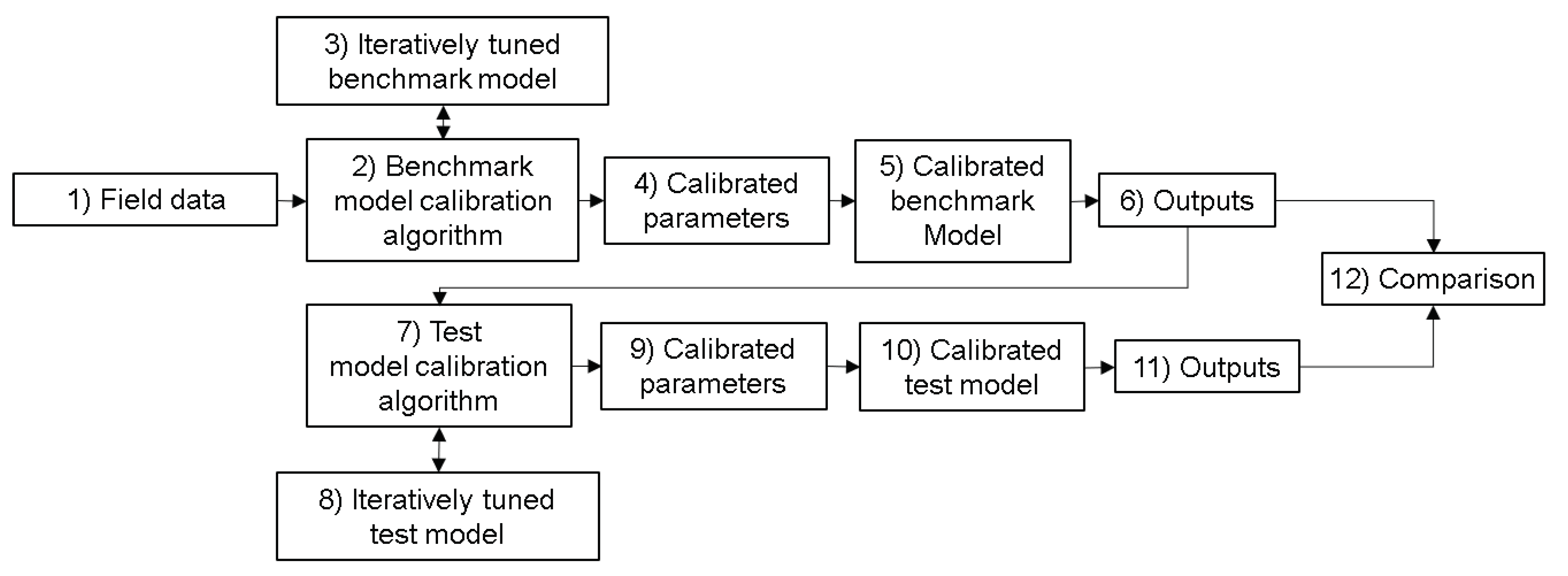
• Develop a framework to compare any two models where high quality field data for calibrating a test model against a benchmark model is not directly available;
• Survey of soil nitrogen models and ranking those based on a number of N-pools and parameters, which are indicative of model complexity;
• Implement and compare a lean N-model [10] against a high-fidelity complex agriculture model RZWQM and measuring the degree of fit as well as a speed-up in simulation time;
• Implement both the lean N-model and the routine for automated calibration in the same programming language for fast interfacing;
• Host the lean soil nitrogen model in MyGeoHub, making the model cloud accessible through a browser and cross-platform, thus eliminating local installation.

In the rest of the paper, we first list and compare some popular soil nitrogen (N) models found in the literature in

Table 1. List of soil Nitrogen (N) models ordered according to decreasing complexity.

#	Name	$\#\mathit{Pools}$ *	$\#\mathit{Params}$ *	Additional Input	Additional Process	Ref. & Remark ${}^{†}$
(1)	SPACSYS	27	45		P cycle; N fixation; 3D root;	Wu et al. [41] (2007) rothamsted.ac.uk/rothamsted-spacsys-model
(2)	RZWQM	19	44		ammonia volatilisation; urea hydrolysis; pesticide; P cycle [42]	Ahuja et al. [31] (2000) ars.usda.gov/plains-area/fort-collins-co/
(3)	DAISY	14	35	GIS		Hansen et al. [43] (1990) daisy.ku.dk/
(4)	CoupModel	12	35	GIS		Liang et al. [44] (2016). N model is based on DAISY
(5)	WHCNS	10	35		ammonia volatilisation;	Jansson [45] (2012) http://www.coupmodel.com/
(6)	ECOSSE	8	35	GIS	methane dynamics;	Smith et al. [46] (2010) abdn.ac.uk/staffpages/uploads/soi450/ECOSSE%20User%20manual%20310810.pdf
(7)	EPIC	12	25		ammonia volatilisation; N fixation; erosion; P cycle; pesticide;	Sharpley and Williams [13] (1990), Gerik et al. [47] (2014) epicapex.tamu.edu/epic/. Inspired from CENTURY [48]
(8)	DNDC	16	20	GIS	methane dynamics; ammonia volatilisation; urea hydrolysis;	Li et al. [49] (1992). dndc.sr.unh.edu/
(9)	SOILN	13	20			Johnsson et al. [50] (1987)
(10)	APEX	12	25		erosion; grazing; pesticide; P cycle; N fixation; ammonia volatilisation; watershed, reservoir, ground water, sediment.	Williams et al. [51] (2006) epicapex.tamu.edu/apex/. Extension of EPIC.
(11)	WNMM	12	15	GIS		Li et al. [52] (2007)
(12)	MONICA	11	14		N fixation; Ammonia Volatilisation; Urea hydrolysis;	Kersebaum [53] (1995), Nendel [54] (2014) https://github.com/zalf-rpm/monica/wiki. Uses DAISY’s C dynamics. Extension of HERMES [55] model.
(13)	CANDY	6	18		soil loosening/compaction; pesticide; ammonia volatilisation;	Franko et al. [56] (1995), Franko et al. [57] (2015) https://www.ufz.de/index.php?de=39503
(14)	A “Lean” Model	8	12		no denitrification;	Porporato et al. [10] 2003

* These numbers are the best available estimates from the literature. ${}^{†}$ All urls accessed on 31 January 2021.

and Section 2. We briefly describe the nitrogen (and carbon) model in RZWQM in Section 3.1. This is followed with the description of a lean nitrogen model [10] in Section 3.2. Model comparison setup in this work is explained in Section 3.3. MyGeoHub cyber-infrastructure to host the lean N-model is briefly described in Section 3.4. Procedure to host the model in MyGeoHub is described in Section 3.4.1. In Section 4 the implemented lean N-model is calibrated and compared with the RZWQM simulated values for daily nitrate and ammonia levels. The paper is discussed and concluded in Section 5 and Section 6, respectively.

2. Review of Soil Nitrogen Models

Almost all soil nitrogen models comprise of several organic and inorganic pools for N and C, where more complex models have a higher number of pools. Carbon dynamics is coupled with nitrogen dynamics due to consideration of organic matter (OM) and the fact that soil mineral N, ammonia and nitrate, are obtained due to OM decay. The plant takes N from the mineral N pool. Table 1 lists soil N-models in decreasing order of complexity as determined by the number of C and N pools (state-variables) and N model parameters used. These models discretize the soil into a number of layers, and the values for pools (state-variables) and N model params listed are for per layer basis. The models are one dimensional (vertical) and simulate on a daily timescale. The common input variables used by the N-models include: soil moisture and water flow, soil temperature, management inputs like fertilization, irrigation, sowing, tillage, and harvest. Soil moisture and temperature in turn depends on soil property and meteorological inputs like air temperature, wind speed, solar radiation, humidity, and rainfall. The N model is integrated with soil water, soil temperature and a crop growth model. The common outputs of the N models include: daily soil nitrate, ammonia, N loss, nitrogen oxide gases. Processes common to all the N models are: organic matter decomposition, mineralization, immobilization, nitrification, denitrification, microbial effect, crop N uptake and N leach. Some models have additional inputs and processes that are listed in Table 1.

There have also been works that compare some select nitrogen models. For instance in [58], fourteen nitrogen turnover models in a soil-crop system were compared. The processes included in the models, their description and the results of simulations carried out with the same data set were compared. In [59], six soil nitrogen cycles were compared and their processes discussed. To compare the accuracy of the models they were run with the same data set. In [60], four soil nitrogen dynamics models’ processes were reviewed, compared, and analyzed with references to the equations used in each model. Works [61,62] have discussed many soil N models. The reaction rates of the soil nitrogen cycle depends on temperature and moisture. The dependency can be modeled by many equations. The work in [63] compared the Q10, the Arrhenius, and a Logistic function as predictors of the temperature dependence of the soil N mineralization rate in soil. The works [64,65] have analyzed different functions describing the effects of soil moisture, temperature, and their interaction on soil nitrogen transformation. To the best of our knowledge, there is no work comparing RZWQM with the Lean model by Porporato et al. [10] as performed in our setting.

3. Materials and Methods

The six macro nutrients that crops need are: nitrogen, carbon, phosphorous, potassium, calcium, magnesium, and sulfer. Among these, nitrogen and carbon are the most important. Nitrogen is required for amines and proteins in plants, whereas carbon is required for carbohydrates and energy for metabolism. Soil contains inorganic soil minerals and dead and living organic matter, which contain nitrogen and carbon. Each form of organic matter maintains its own near-constant C:N ratio. As organic matter decomposes it either becomes another form of organic matter, which is more resistant to decomposition or is consumed by microbes, which then transforms the organic form, and at times also releases carbon dioxide or methane.

While soil has carbon in the form of organic matter, the plant takes carbon from the atmospheric air only. In contrast, while the atmosphere has ample nitrogen, crops can take nitrogen from soil only in its inorganic form, namely, ammonia and nitrate. Mineralization occurs when nitrogen in organic matter changes to inorganic form ammonia through microbial action. Nitrification, another microbial action, then converts ammonia to nitrate. The reverse microbial action of converting inorganic nitrogen to organic form is termed immobilization. The nitrogen in soil can be released from soil to atmosphere by way of denitrification, which is a chemical reaction of conversion of nitrate to $N_2$ and $N_{2}O$.

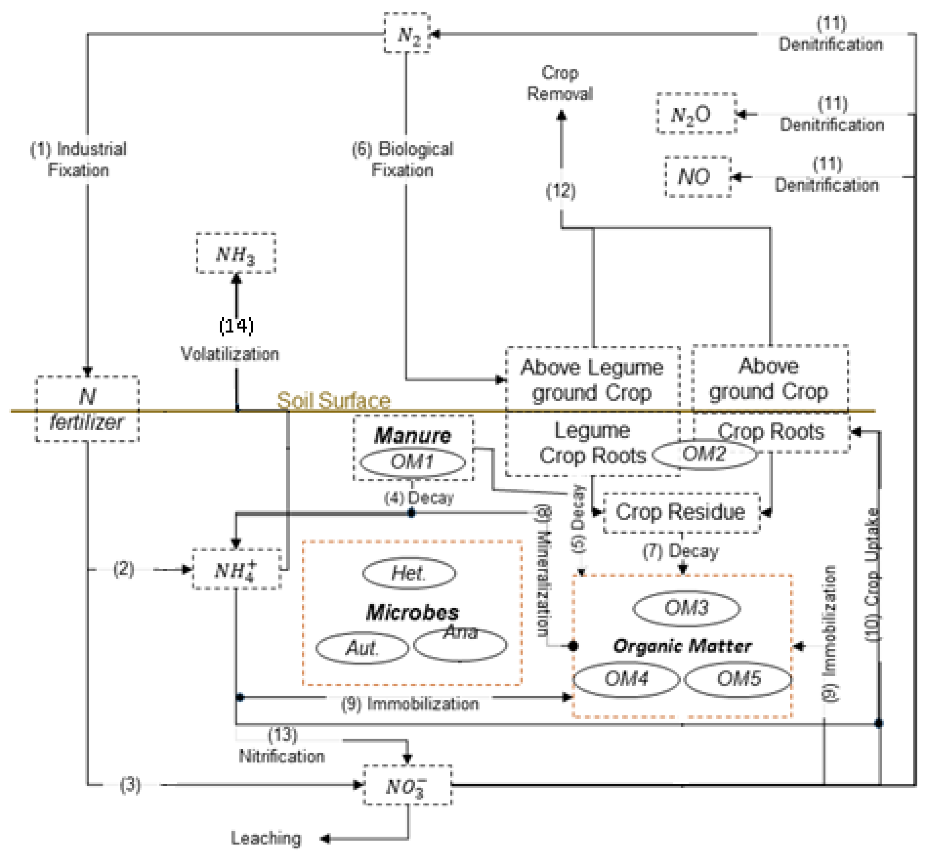
3.1. Soil Nutrient (C and N) Module in RZWQM

The nitrogen cycle in general and as modeled in RZWQM is described below in Figure 1. Here (1) designates the Haber process: $N_2$ + 3$H_2\to 2N{H}_3$ that fixes atmospheric nitrogen to fertilizers, nitrate, ammonia, or urea. (2) indicates the ammonia-containing fertilizer being added to the ammonia pool. Urea, which has two amide groups, converts to ammonium by urea hydrolysis. (3) Indicates the nitrate containing fertilizer being added to the nitrate pool. Nitrate moves downwards, along with water leading to leaching losses. (4) Indicates the slow surface residue pool like manure that is decomposed by heterotrophic bacteria. A fraction of decomposed residual becomes ammonium. (5) Indicates a part of slow surface residue that on decay joins the fast humus pool below the soil surface. (6) Indicates the crops having nitrogen fixing bacteria in root nodules that fixes N from the atmosphere. (7) Indicates the decay of fast surface residue like dead stalks leaves. A fraction of decay matter joins the organic matter (OM) pool below the soil surface. (8) Indicates the decay of OM by bacteria produces ammonium. (9) Indicates the mineral form of N being converted to organic form due to consumption by bacteria. (10) Indicates the crop root uptake of mineral N from soil. (11) Indicates denitrification that causes nitrate to become nitrogen gas. (12) Indicates that the crop N removal via harvesting. (13) Indicates that ammonium converts to nitrate via nitrification by nitrifying bacteria. (14) Volatilization of ammonium to ammonia gas.

The input variables to the C-N system are fertilizer (inorganic N), manure (organic N and C), and soil moisture/temperature/pH. RZWQM has nineteen C and N pools [9], namely, OM pool 1 (slow-decaying structural material), OM pool 2 (fast-decaying metabolic material), OM pool 3 (fast-decaying), OM pool 4 (medium decaying), OM pool 5 (slow decaying), heterotrophic biomass (soil decomposer), autotrophic biomass (nitrifier), heterotrophic biomass (facultative anaerobes), $N{O}_3$, $N{H}_4$, $C{O}_2$ (acts as source or sink), urea, $N_2$ sink, $N{H}_4$ mineralized, $N{O}_3$ immobilized, $N_{2}O$ sink, $N{H}_3$ volatilized, $N{H}_4$ immobilized and $C{H}_4$ (source/sink). Most of the state variables of the system are shown as ellipses and dashed boxes in Figure 1. The dynamics of the first ten state variables are given in Equations (1)–(10). The other remaining pools are used to balance the mass of C and N during transformation of the first ten state variables. RZWQM segregates soil OM into five pools depending on their resistance to decomposition and vicinity to surface. Microbes are divided into three pools. Other simple N models may segregate OM into fewer pools. This transformation among pools is shown by arrows and the corresponding processes mentioned within those arrows. Fertilizer and manure increase the nitrate and ammonia pool by the amount added. Soil water, pH and temperature affect the decay rates of various pools. Flow of water also affects N content through its transport. (Water flow is a separate sub-module in RZWQM.) The outputs, nitrate and ammonia, are available for plant uptake. The carbon content of organic matter pools, as shown in Figure 1, are $C_{OM1}$ for near-surface slow residue pools (e.g., manure), $C_{OM2}$ for near-surface fast residue pools (e.g., crop residue), $C_{OM3}$ for below-surface fast humus pools, $C_{OM4}$ for below-surface intermediate humus pools, $C_{OM5}$ for below-surface slow humus pools, $C_{het}$ for aerobic heterotrophs (organic matter decomposers), $C_{aut}$ for autotrophs or nitrifiers, and $C_{ana}$ for facultative heterotrophs or anaerobic denitrifiers. The nitrogen content of an organic matter pool is obtained by dividing the carbon content with the C:N ratio of that pool. The concentrations of the inorganic pools are $C_{NH4}$ for ammonium, $C_{NH3}$ for ammonia gas, $C_{N03}$ for nitrate, $C_{CO2}$ for carbon dioxide gas, and $C_{N2}$ for nitrogen gas.

The complexity of RZWQM can be gauged by some of the state update equations for the five pools of soil carbon, three pools of microbes, and two pools of mineral nitrogen, as given in the following. These 10 equations and the interrelations among them have been consolidated from [9]. In these equations, the following notations are used: T—soil temperature, $k_b$—Boltzmann constant, $h_p$—Planks Constant, $f_{aer}$—factor for the extent of aerobic conditions (this depends on soil water content and bulk density), $A_i$—pool specific rate coefficient, $E_a$—apparent activation energy, $O_2$—oxygen concentration in soil, H—hydrogen ion concentration, $kh$—hydrogen ion concentration in soil, ${\gamma }_1$—activity coefficient for monovalent ion, $k_h$—hydrogen ion exponent for decay of OM, $e_{max}$, $e_{nit}$—efficiency factor, $f_r$—fraction of soil decomposer over total heterotrophs, $f_t\left(i\right)$—fraction of decayed OMi lost to other OM pools, $C_N$—C:N ratio of autotrophic biomass, $a_{ad}$—decay conversion factor (this depends on soil water content and bulk density), $e_{ad}$—fraction of decayed soil carbon to biomass, $C_S$—weighted carbon substrate concentration (linear combination of OMs), $E_{a}n$—apparent activation energy for nitrification, $E_{death}$—apparent activation energy for microbial death. $R_{ij}$—fraction of decayed OM transferred from pool i to j, $E_{den}$—apparent activation energy for denitrification, $A_{den}$—denitrification rate coefficient, $k_{v0}$—volatilization constant, W—wind speed, Z—soil depth, $P_{NH3}^{\prime }$—soil depth, $C_{urea}$—urea concentration, $E_k$—equilibrium constant between ammonia and ammonium, $A_u$—rate coefficient for urea hydrolysis, $E_u$—activation energy for urea hydrolysis.

Equation (1) below models the decay of the OM1 pool in Figure 1 (paths 4 and 5). Equation (2) models the decay of the OM2 pool (path 7). Equation (3), the decay of the OM3 pool, along with the addition of a fraction of decayed OM2 to OM3 (path 7) and that of dead microbes to OM3. Equation (4) models the decay of the OM4 pool, along with the addition of fractions of decayed OM1 (path 5) and OM3 to OM4. Equation (5) models the decay of the OM5 pool and the conversion of a fraction of decayed OM4 pool into OM5. Equation (6) describes growth of the heterotroph microbe pool (soil decomposers) by consumption of decayed OM pools, and its own death. Equation (8) describes the growth and death of the autotroph microbe pool (nitrifiers). Equation (8) describes the growth of the anaerobe microbe pool (facultative heterotrophs) by feeding on decayed OMs and by denitrifying soil $N{O}_3$, alongside their death. Equation (9) models loss of ammonium due to nitrification (path 13) and volatilization (path 14), and accumulation due to urea hydrolysis if urea fertilizer is added (path 2). If ammonium-containing fertilizer is applied, that amount also gets added to the NH4 pool (path 2). Equation (10) describes accumulation of nitrate due to nitrification (path 13), loss of nitrate by denitrification (path 11), and if nitrate-containing fertilizer is applied, that amount is directly added to the NO3 pool (path 3). If a crop is also present, then root uptake of N diminishes NH4 and NO3 pools (path 19). The N-level of each OM pool is calculated from each pool’s C:N ratio, which are constant and specific to a pool. To maintain mass balance, C is adjusted by release/absorption of $C{O}_2$ (if $O_2$ not limiting) or $C{H}_4$ (if $O_2$ scarce) and N is adjusted by release (mineralization, path 8) or absorption (immobilization, path 9) of $N{H}_4$.

$${\mathrm{C}}_{OM1}[\mathrm{d}+1]={\mathrm{C}}_{OM1}\left[\mathrm{d}\right]-f_{aer}\frac{k_{b}T}{h_p}{A}_1{e}^{\frac{-E_a}{R_{g}T}}\frac{\left[O_2\right]}{\left[H^{kh}{\gamma }_1^{kh}\right]}950C_{het}\left[\mathrm{d}\right]{\mathrm{C}}_{OM1}\left[\mathrm{d}\right]$$

(1)

$${\mathrm{C}}_{OM2}[\mathrm{d}+1]={\mathrm{C}}_{\mathrm{OM}2}\left[\mathrm{d}\right]-f_{\mathrm{aer}}\frac{k_{b}T}{h_p}{A}_2{e}^{\frac{-E_a}{R_{g}T}}\frac{\left[O_2\right]}{\left[H^{kh}{\gamma }_1^{kh}\right]}950C_{\mathrm{het}}\left[\mathrm{d}\right]{\mathrm{C}}_{OM2}\left[\mathrm{d}\right]$$

(2)

$$\begin{array}{cc}\hfill {\mathrm{C}}_{OM3}[\mathrm{d}+1]& ={\mathrm{C}}_{OM3}\left[\mathrm{d}\right]-f_{aer}\frac{k_{b}T}{h_p}{A}_3{e}^{\frac{-E_a}{R_{g}T}}\frac{\left[O_2\right]}{\left[H^{kh}{\gamma }_1^{kh}\right]}950C_{het}\left[\mathrm{d}\right]{\mathrm{C}}_{OM3}\left[\mathrm{d}\right]\hfill \\ \hfill & +{\mathrm{R}}_{23}{f}_{\mathrm{aer}}\frac{k_{b}T}{h_p}{A}_2{e}^{\frac{-E_a}{R_{g}T}}\frac{\left[O_2\right]}{\left[H^{kh}{\gamma }_1^{kh}\right]}950C_{\mathrm{het}}\left[\mathrm{d}\right]{\mathrm{C}}_{OM2}\left[\mathrm{d}\right]\hfill \\ \hfill & +\frac{1}{f_{\mathrm{aer}}}\left(\frac{k_{b}T}{h_p}\right)A_{\mathrm{death},\mathrm{het}}{e}^{\frac{-E_{\mathrm{death},het}}{RgT}}\frac{H{\gamma }_1}{\left[o_2\right]C_S}{\mathrm{C}}_{\mathrm{het}}\left[\mathrm{d}\right]\hfill \\ \hfill & +\frac{1}{f_{aer}}\left(\frac{k_{b}T}{h_p}\right)A_{\mathrm{death},aut}{e}^{\frac{-E_{\mathrm{death},aut}}{Rg}}\frac{H{\gamma }_1}{\left[o_2\right]C_{NH4}\left[d\right]}{\mathrm{C}}_{\mathrm{aut}}\left[\mathrm{d}\right]\hfill \\ \hfill & +\frac{1}{f_{aer}}\left(\frac{k_{b}T}{h_p}\right)A_{\mathrm{death},\mathrm{ana}}{e}^{\frac{-E_{\mathrm{death},\mathrm{ana}}}{R_{g}T}}\frac{H{\gamma }_1}{\left[o_2\right]C_s}{\mathrm{C}}_{\mathrm{ana}}\left[\mathrm{d}\right]\hfill \\ \hfill & +\frac{1}{f_{aer}}\left(\frac{k_{b}T}{h_p}\right)A_{\mathrm{death},ana}{e}^{\frac{-E_{\mathrm{death},\mathrm{ana}}}{R_{g}T}}\frac{H{\gamma }_1}{Cs{C}_{NO3}\left[d\right]}{\mathrm{C}}_{\mathrm{ana}}\left[\mathrm{d}\right]\hfill \end{array}$$

(3)

$$\begin{array}{cc}\hfill {\mathrm{C}}_{\mathrm{OM}4}[\mathrm{d}+1]& ={\mathrm{C}}_{\mathrm{OM}4}\left[\mathrm{d}\right]-f_{\mathrm{aer}}\frac{k_{b}T}{h_p}{A}_4{e}^{\frac{-E_a}{R_{g}T}}\frac{\left[o_2\right]}{\left[H^{kh}{\gamma }_1^{kh}\right]}950C_{het}\left[\mathrm{d}\right]{\mathrm{C}}_{OM4}\left[\mathrm{d}\right]\hfill \\ \hfill & +{\mathrm{R}}_{14}{f}_{\mathrm{aer}}\frac{k_{b}T}{h_p}{A}_1{e}^{\frac{-E_a}{R_{g}T}}\frac{\left[o_2\right]}{\left[H^{kh}{\gamma }_1^{kh}\right]}950C_{\mathrm{het}}\left[\mathrm{d}\right]{\mathrm{C}}_{OM1}\left[\mathrm{d}\right]\hfill \\ \hfill & +{\mathrm{R}}_{34}{f}_{\mathrm{aer}}\frac{k_{b}T}{h_p}{A}_3{e}^{\frac{-E_a}{R_{g}T}}\frac{\left[o_2\right]}{\left[H^{kh}{\gamma }_1^{kh}\right]}950C_{\mathrm{het}}\left[\mathrm{d}\right]{\mathrm{C}}_{OM3}\left[\mathrm{d}\right]\hfill \end{array}$$

(4)

$$\begin{array}{cc}\hfill {\mathrm{C}}_{\mathrm{OM}5}[\mathrm{d}+1]& ={\mathrm{C}}_{OM5}\left[\mathrm{d}\right]-f_{\mathrm{aer}}\frac{k_{b}T}{h_p}{A}_5{e}^{\frac{-E_a}{R_{g}T}}\frac{\left[o_2\right]}{\left[H^{kh}{\gamma }_1^{kh}\right]}950C_{\mathrm{het}}\left[\mathrm{d}\right]{\mathrm{C}}_{OM5}\left[\mathrm{d}\right]\hfill \\ \hfill & +{\mathrm{R}}_{45}{f}_{\mathrm{aer}}\frac{k_{b}T}{h_p}{A}_4{e}^{\frac{-E_a}{R_{g}T}}\frac{\left[o_2\right]}{\left[H^{kh}{\gamma }_1^{kh}\right]}950C_{het}\left[\mathrm{d}\right]{\mathrm{C}}_{OM4}\left[\mathrm{d}\right]\hfill \end{array}$$

(5)

$$\begin{array}{cc}\hfill C_{\mathrm{het}}[\mathrm{d}+1]& ={\mathrm{C}}_{\mathrm{het}}\left[\mathrm{d}\right]+\sum _{i=1}^5\left((1-ft\left(i\right)){\mathrm{e}}_{max}\mathrm{fr}{f}_{\mathrm{aer}}\frac{k_{b}T}{h_p}{A}_i{e}^{\frac{-E_a}{R_{g}T}}\frac{\left[o_2\right]}{\left[H^{kh}{\gamma }_1^{kh}\right]}950C_{het}\left[\mathrm{d}\right]C_{OMi}\left[\mathrm{d}\right]\right)\hfill \\ \hfill & -\frac{1}{f_{\mathrm{aer}}}\left(\frac{k_{b}T}{h_p}\right)A_{\mathrm{death},het}{e}^{\frac{-E_{\mathrm{death},het}}{R_{g}T}}\frac{H{\gamma }_1}{\left[o_2\right]C_s}{\mathrm{C}}_{\mathrm{het}}\left[\mathrm{d}\right]\hfill \end{array}$$

(6)

$$\begin{array}{cc}\hfill {\mathrm{C}}_{\mathrm{aut}}[\mathrm{d}+1]& ={\mathrm{C}}_{\mathrm{aut}}\left[\mathrm{d}\right]+e_{nit}{C}_N{f}_{\mathrm{aer}}\frac{k_{b}T}{h_p}{A}_{nit}{e}^{\frac{-E_{an}}{R_{g}T}}\frac{\sqrt{\left[O_2\right]}}{\left[H^{kh}{\gamma }_1^{kh}\right]}9500C_{\mathrm{aut}}\left[\mathrm{d}\right]\hfill \\ \hfill & -\frac{1}{f_{aer}}\left(\frac{k_{b}T}{h_p}\right)A_{\mathrm{death},aut}{e}^{\frac{-E_{\mathrm{death},aut}}{R_{g}T}}\frac{H{\gamma }_1}{\left[0_2\right]C_{NH4}\left[d\right]}{\mathrm{C}}_{\mathrm{aut}}\left[\mathrm{d}\right]\hfill \end{array}$$

(7)

$$\begin{array}{cc}\hfill {\mathrm{C}}_{\mathrm{ana}}[\mathrm{d}+1]& ={\mathrm{C}}_{\mathrm{ana}}\left[\mathrm{d}\right]+\sum _{i=1}^5\left((1-ft\left(i\right)){\mathrm{e}}_{max}(1-\mathrm{fr})f_{\mathrm{aer}}\frac{k_{b}T}{h_p}{A}_i{e}^{\frac{-E_a}{R_{g}T}}\frac{\left[O_2\right]}{\left[H^{kh}{\gamma }_1^{kh}\right]}950C_{het}\left[\mathrm{d}\right]C_{OMi}\left[\mathrm{d}\right]\right)\hfill \\ \hfill & +e_{ad}{a}_{ad}{f}_{\mathrm{anaer}}\frac{k_{b}T}{h_p}{A}_{\mathrm{den}}{e}^{\frac{-E_{\mathrm{den}}}{R_{g}T}}\frac{c_s}{\left[H^{kh}{\gamma }_1^{kh}\right]}9500C_{\mathrm{ana}}\left[d\right]C_{NO3}\left[\mathrm{d}\right]\hfill \\ \hfill & -\frac{1}{f_{aer}}\left(\frac{k_{b}T}{h_p}\right)A_{\mathrm{death},ana}{e}^{\frac{-E_{\mathrm{death},\mathrm{ana}}}{RgT}}\frac{H{\gamma }_1}{\left[o_2\right]C_s}{\mathrm{C}}_{\mathrm{ana}}\left[\mathrm{d}\right]\hfill \\ \hfill & -\frac{1}{\mathrm{fanaer}}\left(\frac{k_{b}T}{h_p}\right)A_{\mathrm{death},\mathrm{ana}}{e}^{\frac{-E_{\mathrm{death},\mathrm{het}}}{RgT}}\frac{H{\gamma }_1}{{\mathrm{C}}_{\mathrm{NO}3}\left[d\right]C_S}{\mathrm{C}}_{\mathrm{ana}}\left[\mathrm{d}\right]\hfill \end{array}$$

(8)

$$\begin{array}{cc}\hfill {\mathrm{C}}_{\mathrm{NH}4}[\mathrm{d}+1]& ={\mathrm{C}}_{\mathrm{NH}4}\left[\mathrm{d}\right]-f_{aer}\frac{k_{b}T}{h_p}{A}_{nit}{e}^{\frac{-E_{an}}{RgT}}\frac{\left[o_2\right]}{\left[H^{kh}{\gamma }_1^{kh}\right]}9500C_{aut}\left[\mathrm{d}\right]\hfill \\ \hfill & -k_{v0}log\left(W\right)e^{-0.25Z}{T}_{k1}{e}^{\frac{-0.6}{T_{k2}(T+273)}}\left(\frac{E_k{C}_{NH4}\left[d\right]}{\left[H\right]}-P_{NH3}^{\prime }\right)C_{NH4}\left[\mathrm{d}\right]\hfill \\ \hfill & +2f_{aer}\left(\frac{k_{b}T}{h_p}\right)A_u{e}^{\frac{-E_u}{RgT}}{\mathrm{C}}_{\mathrm{urea}}\left[d\right]\hfill \end{array}$$

(9)

$$\begin{array}{cc}\hfill {\mathrm{C}}_{\mathrm{NO}3}[\mathrm{d}+1]& ={\mathrm{C}}_{\mathrm{NO}3}\left[\mathrm{d}\right]+f_{aer}\frac{k_{b}T}{h_p}{A}_{nit}{e}^{\frac{-E_{an}}{RgT}}\frac{\left[o_2\right]}{\left[H^{kh}{\gamma }_1^{kh}\right]}9500C_{aut}\left[\mathrm{d}\right]\hfill \\ \hfill & -f_{\mathrm{anaer}}\frac{k_{b}T}{h_p}{A}_{\mathrm{den}}{e}^{\frac{-E_{\mathrm{den}}}{R_{g}T}}\frac{c_s}{\left[H^{kh}{\gamma }_1^{kh}\right]}9500C_{\mathrm{ana}}\left[\mathrm{d}\right]C_{\mathrm{NO}3}\left[\mathrm{d}\right]\hfill \end{array}$$

(10)

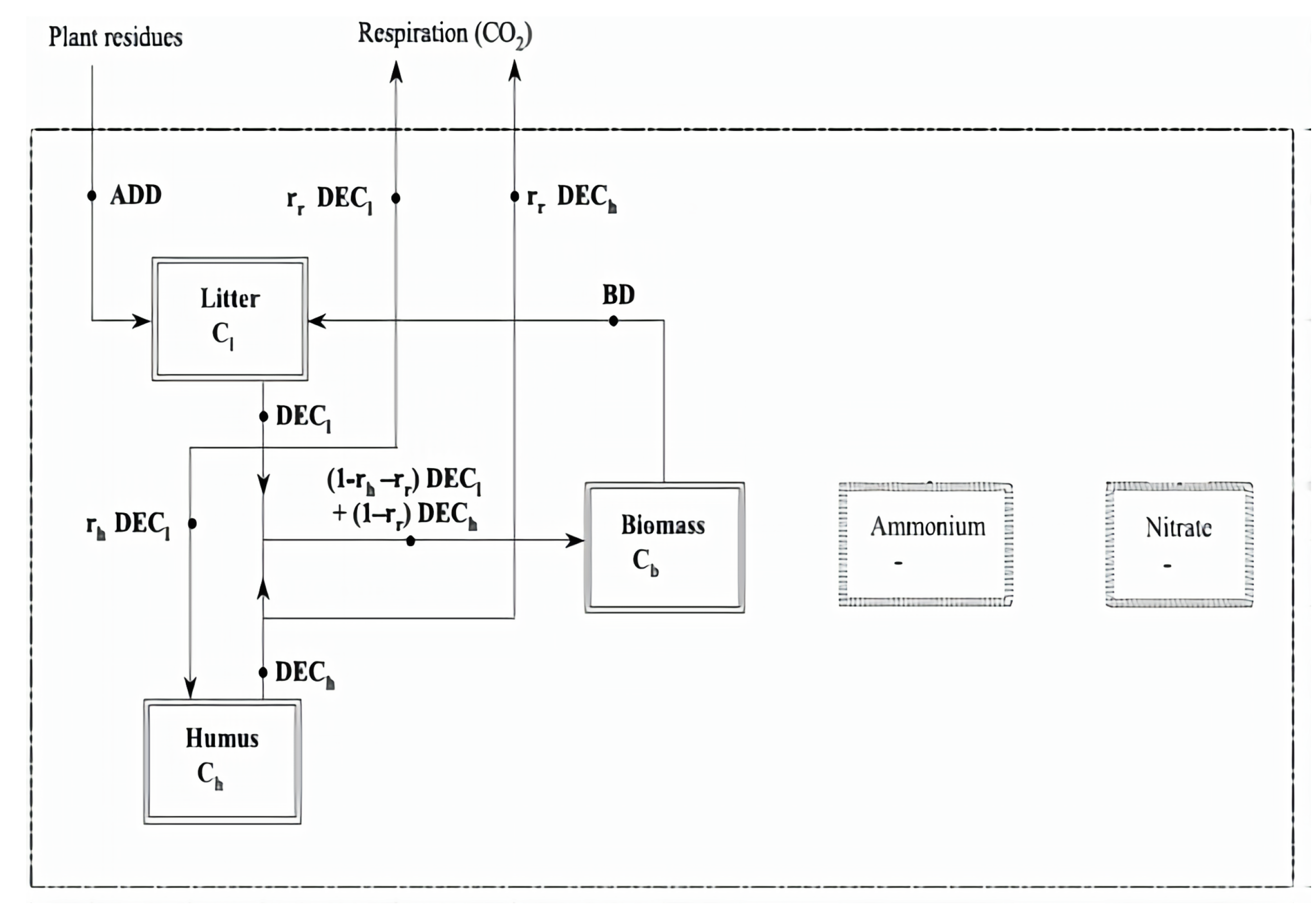
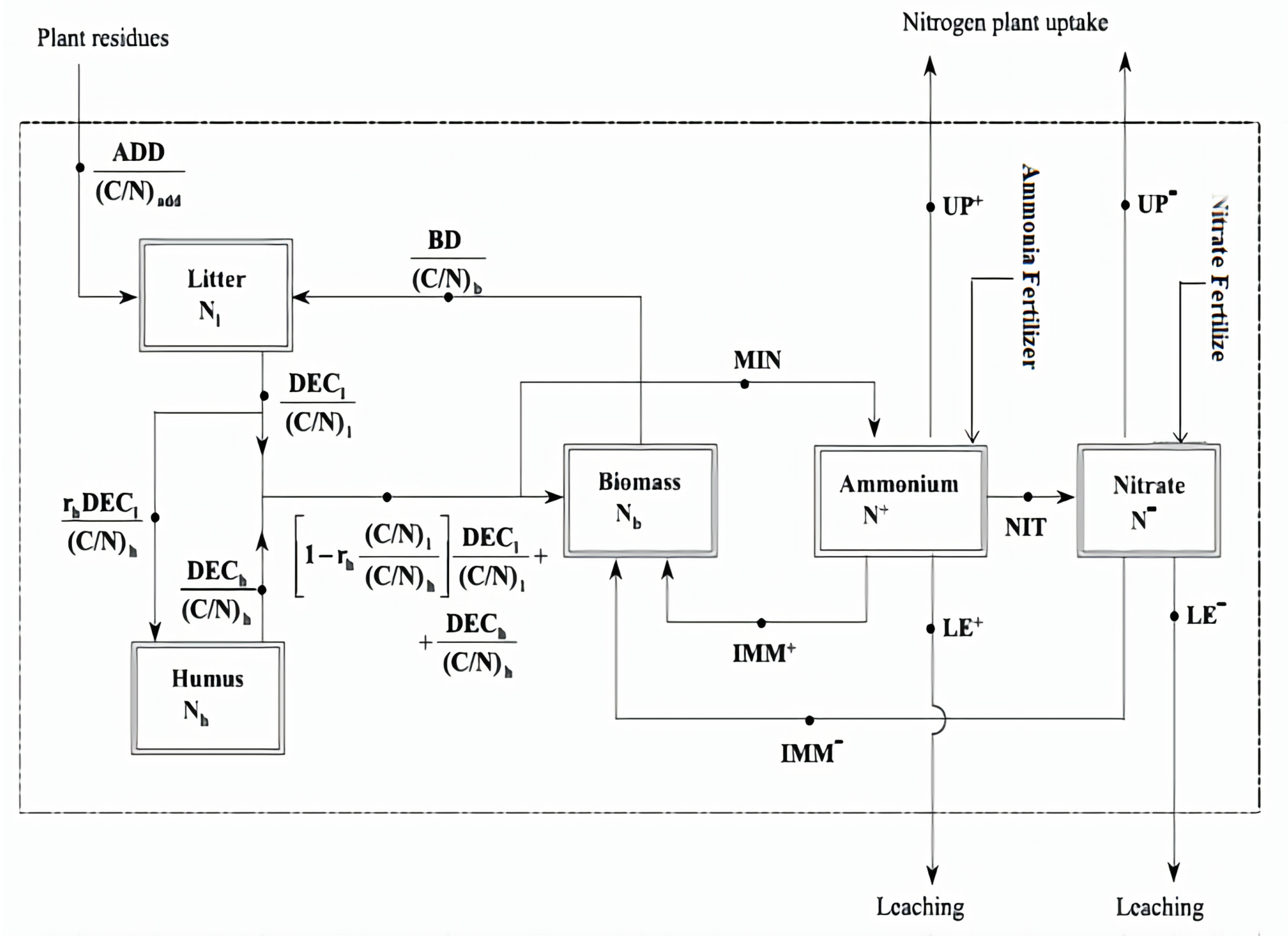
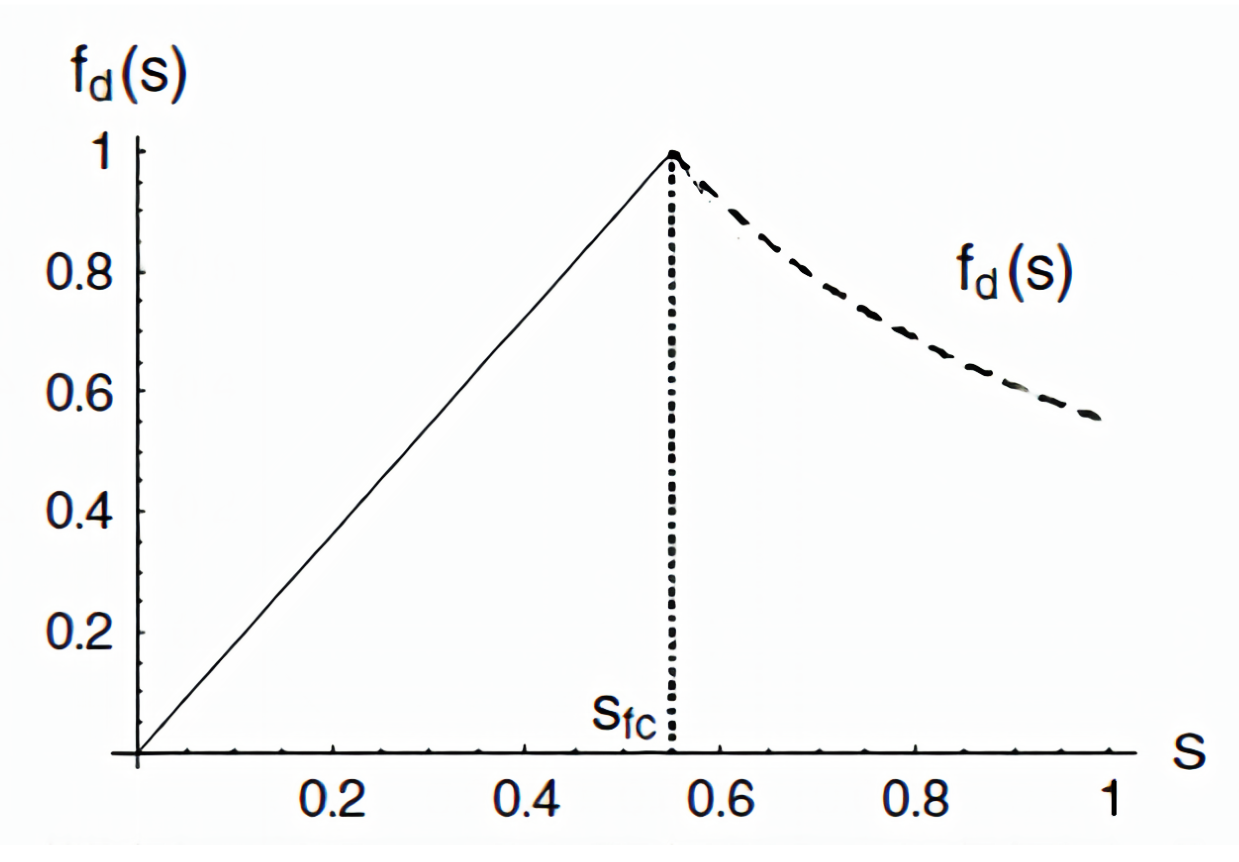
3.2. A Lean Nutrient Model

While the RZWQM model represents the upper extreme of complexity, an alternative lean nutrient model is desirable as explained in the Introduction. For this, we implemented the model taken from [10] and provide its comparison with RZWQM. This lean model makes certain simplifying assumptions: there are no volatilizations of ammonium to ammonia, no ammonia absorption, no nitrogen deposition from the atmosphere, no biological fixation of nitrogen, no denitrification of nitrate to nitrogen gas. Furthermore, only one soil layer of 200 cm depth is considered instead of the seven soil layers in RZWQM.

Figure 2 and Figure 3 show the same set of pools, but Figure 2 shows the carbon fluxes, while Figure 3 shows the N fluxes. Plants uptake mineral nitrogen, in the form of ammonium ($N{H}_4$) and nitrate ($N{O}_3$), which are made available through OM decomposition. That is why the nitrogen cycle is closely linked to that of carbon. As can be seen from Figure 1 and Figure 2, the lean model has one litter pool in contrast to two residue pools in RZWQM, while the three soil humus pools of RZWQM are replaced with a single humus pool. Furthermore, only one microbial biomass pool is used against the three microbial pools of RZWQM. All the pools maintain a constant C:N ratio: whenever there is a flux of carbon between pools there is a commensurate flux of nitrogen between pools also.

In Figure 2, a fraction $r_h$ of decayed litter (in the form of carbon) goes to the humus pool and a fraction $r_r$ is respired as $C{O}_2$. The remaining carbon is consumed by microbes for their growth. The humus pool on decomposition goes to the microbes pool and respires as $C{O}_2$ to the atmosphere. In Figure 3, there are various additional fluxes that impact the nitrogen pool; namely, (i) MIN flux flow of nitrogen from organic matter pool to the mineral N pool, which happens when the litter and humus have more nitrogen, (ii) IMM flux that accounts for immobilization; this flux happens when there is insufficient nitrogen for microbial growth and the microbes consume inorganic nitrogen in the form of ammonia and nitrate. Ammonia and nitrate can leach and flow out of the soil profile. Ammonia and nitrate can have an incoming flux of nitrogen when fertilizers are added, and those can also be taken up by the crop roots.

The rate equation for carbon content in the litter pool is given by (11), where t is timestamp; $ADD$ is external input into the system:

$$\frac{d{C}_l}{dt}=ADD\left[t\right]+BD\left[t\right]-DECl\left[t\right],$$

(11)

where in (11), the microbial biomass death $BD$ is given as:

$$BD\left[t\right]=k_d{C}_b\left[t\right],$$

(12)

in which $C_b$ is the carbon concentration in the microbial biomass pool and $k_d$ is a proportionality constant. Decay of litter $DECl$ by microbes is given as:

$$\mathrm{DECl}\left[\mathrm{t}\right]=\rho \left[t\right]f_d\left(s\left[t\right]\right)k_l{C}_b\left[t\right]C_l\left[t\right],$$

(13)

where $C_l$ is carbon concentration in the litter pool, $k_l$ is proportionality constant (defines the rate of decomposition for the litter pool), coefficient $\rho$ (with $0\le \rho \le 1$ and 0 implying not enough mineral N for immobilization) is a factor that accounts for reduction of the decomposition rate when the litter is very poor in nitrogen and the immobilization is not sufficient to integrate the nitrogen required by the bacteria, s is relative soil moisture, and the soil moisture factor on decay $f_d$ is given as:

$$f_d\left(s\left[t\right]\right)=\left\{\begin{array}{cc}\frac{s\left[t\right]}{s_{fc}}\hfill & s\left[t\right]\le s_{fc}\hfill \\ \frac{s_{fc}}{s\left[t\right]}\hfill & s\left[t\right]>s_{fc},\hfill \end{array}\right.$$

(14)

in which $S_{fc}$ is the normalized field capacity. The variation of $f_d$ is given below in Figure 4.

The dynamics for the nitrogen component of the litter is as follows:

$$\frac{d{N}_l}{dt}=\frac{ADD\left[t\right]}{{(C/N)}_{add}}+\frac{BD\left[t\right]}{{(C/N)}_b}-\frac{DECl\left[t\right]}{{\left(\frac{C}{N}\right)}_l}.$$

(15)

where ${(C/N)}_{add}$, ${(C/N)}_b$ and ${(C/N)}_l$ are C:N ratios of the added plant residue, microbe and litter pools, respectively. The equation for carbon content of the humus pool is:

$$\frac{d{C}_h}{dt}=r_{h}DECl\left[t\right]-DECh\left[t\right],$$

(16)

where $r_h$ is the isohumic coefficient. In (16) the decay rate of humus carbon is given as:

$$DECh\left[t\right]=\rho \left[t\right]f_d\left(s\left[t\right]\right)k_h{C}_b\left[t\right]C_h\left[t\right],$$

(17)

in which proportionality constant $k_h\ll k_l$. The equation for the nitrogen content of the humus pool is:

$$\frac{d{N}_h}{dt}=r_h\frac{DECl\left[t\right]}{{(C/N)}_h}-\frac{DECh\left[t\right]}{{\left(\frac{C}{N}\right)}_h}.$$

(18)

The rate equation for the carbon in microbial pool is:

$$\frac{d{C}_b}{dt}=\left(1-r_h-r_r\right)DECl\left[t\right]+\left(1-r_r\right)DE{C}_h\left[t\right]-BD\left[t\right].$$

(19)

The rate equation balance for nitrogen in the microbial pool is:

$$\frac{d{N}_b}{dt}=\left[1-r_h\frac{{(C/N)}_l}{{(C/N)}_h}\right]\frac{DECl\left[t\right]}{{(C/N)}_l}+\frac{DECh\left[t\right]}{{(C/N)}_h}-\frac{BD\left[t\right]}{{\left(\frac{C}{N}\right)}_b}-\varphi \left[t\right],$$

(20)

where $\varphi \left[t\right]$ is the net mineralization given as:

$$\varphi \left[t\right]=MIN-IMM$$

(21)

$$IMM\left[t\right]=IM{M}^{+}\left[t\right]+IM{M}^{-}\left[t\right],$$

(22)

where $MIN$ is gross mineralization, $IMM$ is the total rate of immobilization, $IM{M}^{+}$ is the immobilization rate of ammonium and $IM{M}^{-}$ is the immobilization rate of nitrate. Net mineralization (i.e., $\varphi >0$), implies $IMM=0$ and $MIN=\varphi$, whereas net immobilization (i.e., $\varphi <0$), implies $MIN=0$ and $IMM=\varphi$. Accordingly, three possible cases might arise depending on nitrogen availability:

Case I: If litter and humus have sufficient N to keep ${(C/N)}_b$ constant, then net mineralization.

Case II: If litter and humus have insufficient N, then microbes consume N from the mineral pool, i.e., the case of immobilization.

Case III: If litter, humus, and mineral N have insufficient N, the decay is slowed down by reducing $\rho$. The mathematical equivalents of the three cases are as follows:

If $\left\{k_h{C}_h\left[\frac{1}{{(C/N)}_h}-\frac{1-r_r}{{(C/N)}_b}\right]+k_l{C}_l\left[\frac{1}{{(C/N)}_l}-\frac{r_h}{{\left(\frac{C}{N}\right)}_h}-\frac{1-r_h-r_r}{{(C/N)}_b}\right]\right\}>0$, then Case I and $\rho =1$.

If $\left\{k_h{C}_h\left[\frac{1}{{(C/N)}_h}-\frac{1r_r}{{(C/N)}_b}\right]+k_l{C}_l\left[\frac{1}{{(C/N)}_l}-\frac{r_h}{{\left(\frac{C}{N}\right)}_h}-\frac{1r_h{r}_r}{{(C/N)}_b}\right]\right\}<0$, then immobilization, and if $IMM\le IM{M}_{max}$, then Case II with $\rho =1$, where immobilization of ammonia and nitrate given as:

$$IM{M}^{+}=\frac{k_i^{+}{N}^{+}}{k_i^{+}{N}^{+}+k_i^{-}{N}^{-}}IMM,\mathrm{and}$$

(23)

$$IM{M}^{-}=\frac{k_i^{-}{N}^{-}}{k_i^{+}{N}^{+}+k_i^{-}{N}^{-}}IMM,\mathrm{and}$$

(24)

with

$$IM{M}_{max}=\left(k_i^{+}{N}^{+}+k_i^{-}{N}^{-}\right)f_d\left(s\left[t\right]\right)C_b\left[t\right],\mathrm{and}$$

(25)

$$IMM=\mid \rho f_d\left(s\left[t\right]\right)C_b\left[t\right]\left\{k_h{C}_h\left[\frac{1}{{(C/N)}_h}-\frac{1-r_r}{{(C/N)}_b}\right]+k_l{C}_l\left[\frac{1}{{(C/N)}_l}-\frac{r_h}{{\left(\frac{C}{N}\right)}_h}-\frac{1-r_h-r_r}{{(C/N)}_b}\right]\right\}.$$

(26)

Otherwise, Case III with

$$\rho =\left|\begin{array}{c}\left(k_i^{+}{N}^{+}+k_i^{-}{N}^{-}\right)\hfill \\ /\left(k_h{C}_h\left[\frac{1}{{(C/N)}_h}-\frac{1-r_r}{{(C/N)}_b}\right]+k_l{C}_l\left[\frac{1}{(C/N)l}-\frac{r_h}{{\left(\frac{C}{N}\right)}_h}-\frac{1-r_h-r_r}{{(C/N)}_b}\right]\right)\hfill \end{array}\right|.$$

(27)

The equations for nitrate and ammonia dynamics are:

$$\frac{d{N}^{+}}{dt}=MIN-IM{M}^{+}-NIT-L{E}^{+}+\mathrm{Ammonia}\mathrm{Fertilizer}\left[t\right],\mathrm{and}$$

(28)

$$\frac{d{N}^{-}}{dt}=NIT-IM{M}^{-}-L{E}^{-}+\mathrm{Nitrate}\mathrm{Fertilizer}\left[t\right],$$

(29)

with nitrification given as:

$$NIT=f_n\left(s\left[t\right]\right)k_n{C}_b\left[t\right]N^{+}\left[t\right].$$

(30)

The moisture factor on nitrification is given by:

$$f_n\left(s\left[t\right]\right)=\left\{\begin{array}{cc}\frac{s\left[t\right]}{s_{fc}}& s\left[t\right]\le s_{fc}\hfill \\ \frac{1-s\left[t\right]}{1-s_{fc}}& s\left[t\right]>s_{fc}\hfill \end{array}\right.\mathrm{and}$$

(31)

the leaching of ammonia and nitrate is given by:

$$L{E}^{\pm }=a^{\pm }\frac{L\left(s\right[t\left]\right)}{s\left[t\right]n{Z}_r}{N}^{\pm },$$

(32)

in which the water flow leaching downward is:

$$L\left(s\left[t\right]\right)=\frac{K_S}{e^{\beta \left(1-s_{fc}\right)}-1}\left[e^{\beta \left(s\left[t\right]-s_{fc}\right)}-1\right],$$

(33)

where $s\left[t\right]$ is soil moisture content at tth day; $a^{\pm }$ is the mixing coefficient of ammonia and nitrate with water; n is soil porosity; $Z_r$ is depth of soil profile; $k_n$ is nitrification constant; $k_l$ is decay constant for kitter pool; $k_h$ is decay constant for humus pool; $k_d$ is death rate of microbes; $K_S$ is saturated hydraulic conductivity; and ${(C/N)}_l$, ${(C/N)}_b$ and ${(C/N)}_h$ are C:N ratios of litter, biomass and humus pool. We can observe that the lean model’s reaction rates do not depend on temperature, unlike RZWQM where reaction rate depends on temperature, pH, soil $O_2$ as well as moisture.

3.3. RZWQN vs. Lean Model Comparison Setup

Due to unavailability of high-frequency agriculture field nitrogen data, we first calibrate RZWQM using the available data from an experimental field in Greeley, CO, and next use the daily nitrate and ammonia data generated from RZWQM as ground truth, against which the lean model’s N dynamics parameters are calibrated. The experimental field is the Limited Irrigation Research Field, a USDA research site, where maize was grown from 2008–2011 with different irrigation treatment. Urea Ammonium Nitrate (UAN) was applied so that there is no N stress. Details of the field experiment can be found in [66]. RZWQM was calibrated to this field as per our prior work [37,67]. Once calibrated, the crop growth was zeroed out in the model since our goal is to compare only the N dynamics. With this, the RZWQM only has active modules for soil N, soil water, and heat dynamics, which were run under normal fertilizer and irrigation application. The run yielded the daily soil water content and nitrate and ammonium values at seven soil depths. The average of these data across the seven depths was then treated as ground truth for calibrating the lean N-model. The lean model requires soil moisture values as can be seen from Equations (13), (30) and (32), but it does not have a coupled soil moisture model. The daily soil water content from RZWQM (averaged over seven soil layer of RZWQM) was given as soil moisture input to the lean N-model. The N dynamic’s parameters listed in

Table 2. Calibrated nutrient parameters’ values for the lean N-model.

Parameter	Lower Range	Calibrated Value	Upper Range
$a^{-}$	0.5	0.943	1.0
$a^{+}$	0.0001	0.0787	0.1
b	1	6.05	13
$K_S$	0.01	0.6647	2.2
$r_h$	0.01	0.01	0.99
$r_r$	0.01	0.322	0.99
$k_d$	0.0001	0.0185	0.0999
$k_l$	$1.0\times {10}^{-6}$	$9.899\times {10}^{-5}$	$9.9\times {10}^{-5}$
$k_h$	$1.0\times {10}^{-7}$	$9.337\times {10}^{-6}$	$9.9\times {10}^{-6}$
$k_n$	0.0001	0.0047	0.9999
$k_i^{+}$	0.1	0.482	1.1
$k_i^{-}$	0.1	0.405	1.1

were calibrated using pyswarm Particle Swarm Optimization package in Python, to fit the ammonium and nitrate data obtained from field calibrated RZWQM. The calibrated lean N model’s ammonium and nitrate output were compared with RZWQM’s, as reported in Section 4.

We next describe our framework for comparing a “test model” (a lean N-model in our case) against a “benchamrk model” (RZWQM N model in our case) when the dataset available is not directly usable by the “test model”. This is because the benchmark model would be embedded within a complete agriculture model and can be calibrated by the available dataset. This more complete model is used to first calibrate its embedded benchmark model, and next the simulation of the benchmark model is used to generate the data needed to calibrate the test model. The proposed framework for this is shown in Figure 5.

The field data (1) is utilized by a calibration program (2) to calibrate a benchmark model embedded within a complete agriculture model (3). The program (2) makes calls to the benchmark model (3) to explore parameter values that best fit the benchmark model to the field data. The program (2) outputs the calibrated parameters (4). With these parameters, the calibrated benchmark model (5) outputs the required data (6) to be able to calibrate the test model. The type of outputs in (6) can differ from that of the field data (1). The output data in (6) is used by program (7) to calibrate a test model (8), again using iterative exploration. The calibrated parameters (9) given by (7) is used by the calibrated test model (10) to give its own outputs (11) of the same variables as in (6). At this point the two model outputs will be compared in (12).

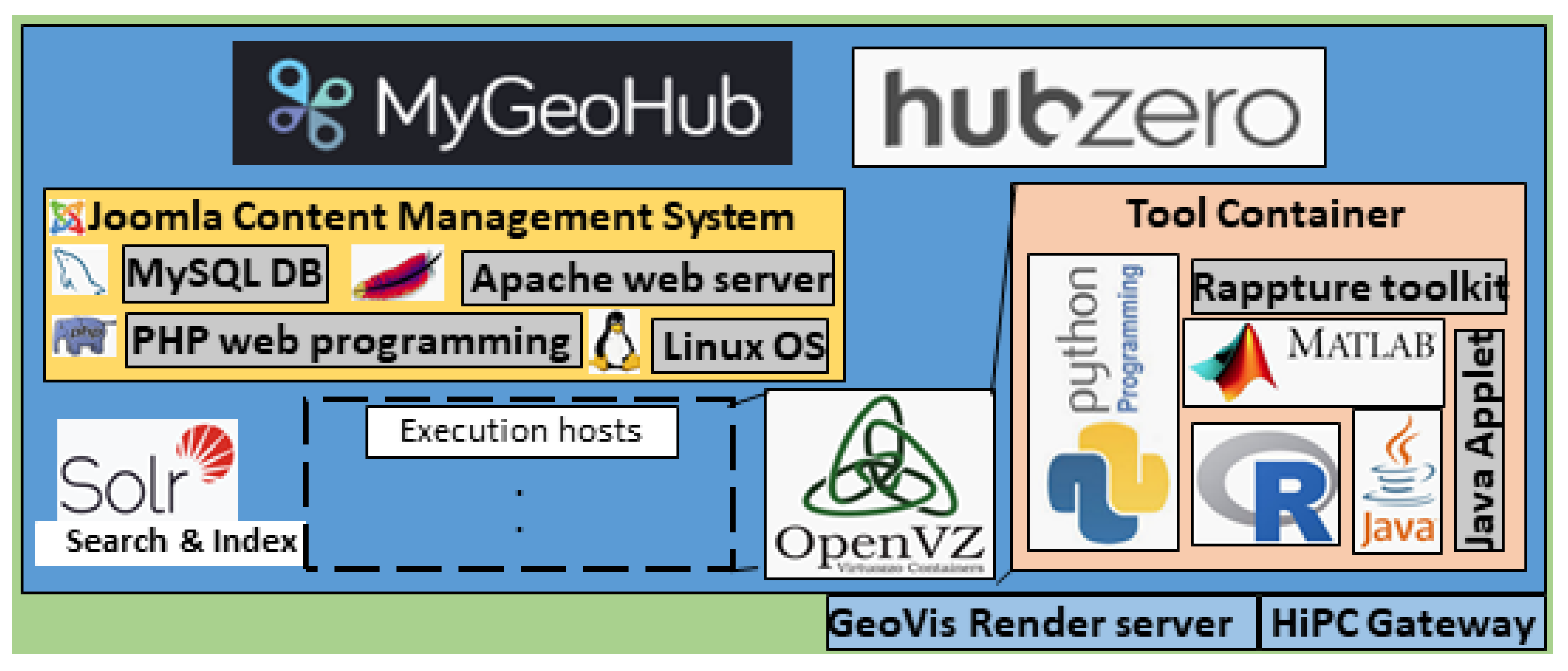
3.4. MyGeoHub Cyber-Infrastructure

Several cyberinfrastructures exist for supporting a variety of disciplines and communities. For instance, TeraGrid [68,69] provides distributed computing, storage and networking facilities to many scientific disciplines. nanoHUB [70] infrastructure is geared for nanotechnology. Integrated computational materials engineering (ICME) [71] cyberinfrastructure supports the manufacturing and materials science community. A cyberinfrastructure for US plant and life science community, formerly iPlant and now renamed as cyverse [72], also exists. An infrastructure for a geographical soil moisture dataset is also being developed [73]. The Hydroshare [74] environment helps the collaboration and sharing of hydrologic data and models. Hubzero (the one we propose to use) [40] lets users access and share tools, data-sets, videos, and tutorials with DOIs (digital object identifiers) for subsequent citations and collaborate online to develop simulation and modeling tools. Numerous scientific communities like pharmaceutical engineering (pharmaHUB.org), heat transfer (https://nanohub.org/groups/thermal (accessed on 28 March 2021)), healthcare (https://indianactsi.org/ (accessed on 28 March 2021)), and geospatial projects (https://mygeohub.org (accessed on 28 March 2021)) use the Hubzero platform.

For this work of implementing a lean N-model as a cloud service, we utilize MyGeoHub [39] infrastructure leveraging Hubzero [40]. MyGeoHub system architecture is depicted in Figure 6. MyGeoHub lets us create collaborative applications that are built from open source software like Linux OS, Apache web server, MySQL database, Joomla content management system, and PHP web scripting. It has built-in support/ticket features, statistics of usage, integration with GitHub/Google Drive/Dropbox, and supports wiki style documentation. Users access interactive and graphical tools via Java applet in their Web browsers. Hub tools run in OpenVZ containers and utilize VNC (Virtual Network Computing) to provide interactive access. The tools run on HPC clusters where jobs can be dispatched to more powerful computers in the national grid infrastructure. The Rappture toolkit generates GUI based on XML description for a tool’s inputs and outputs. The underlying simulator may be written in any programming language. Tool development on the hub is done in the “Workspace” tool, which provides a complete Linux environment. Apart from standard libraries, domain-specific libraries can also be imported.

MyGeoHub hosts four projects, namely, (i) driNET—for sharing local to regional drought information, (ii) WaterHub—for sharing hydrologic information, (iii) Useful-to-Usable (U2U)—to transform historical climate data, knowledge, and model into decision support tools for crop farmers, educators, and Ag advisors, and (iv) Geoshare—to develop a spatially global database on agriculture integrated with an economic analysis tool. Some AgMIP [75] projects use MyGeoHub for hosting its tools. iData in MyGeoHub provides support for the entire cycle of geospatial data driven analysis, management, preview, map search, sharing, and publication. MyGeoHub is free to host and access tools for broad research and education communities.

MyGeoHub requires the file system in the repository to be organized in a particular fashion. The general file setup is as follows. The root folder of the tool repository would have three folders; namely, (i) bin folder, which would have the executable file. This executable file will be run on MyGeoHub when the tool is launched. (ii) The middleware folder that has an invoke file. Invoke file is a bash script that gets the tool ready to run. (iii) The src folder having three subfolders, (a) Source code for the tool (b) Manifest file—file used in the makefile that aids in the compilation of the source code and (c) Makefile—a makefile basically automates the compilation of source code and the creation of an executable file.

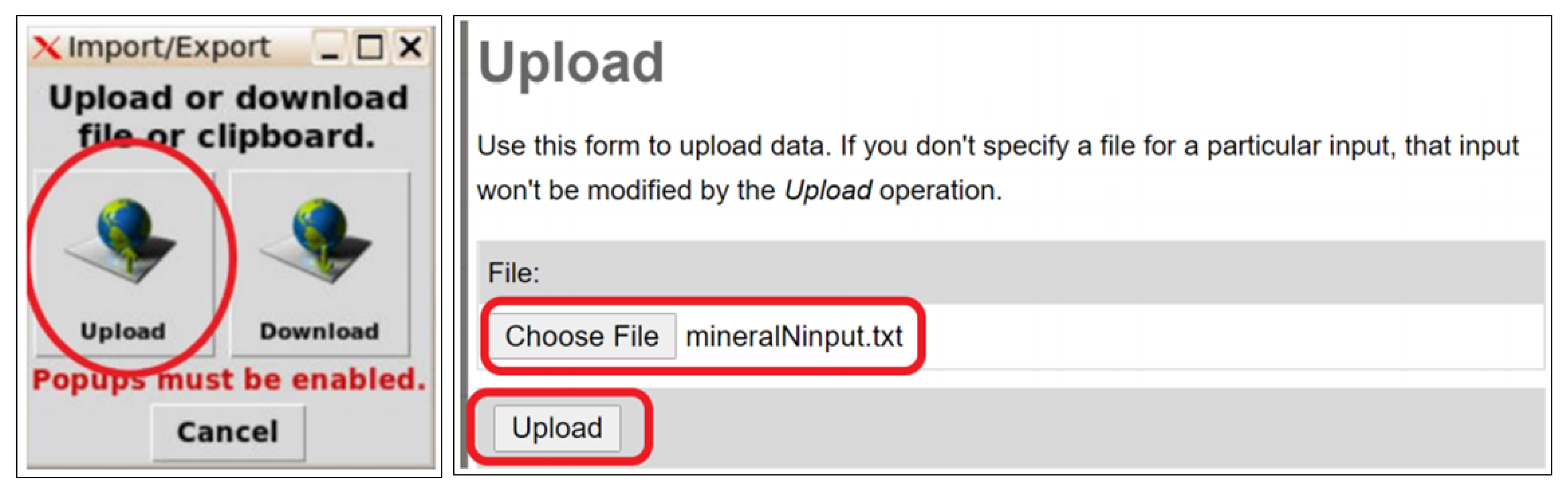
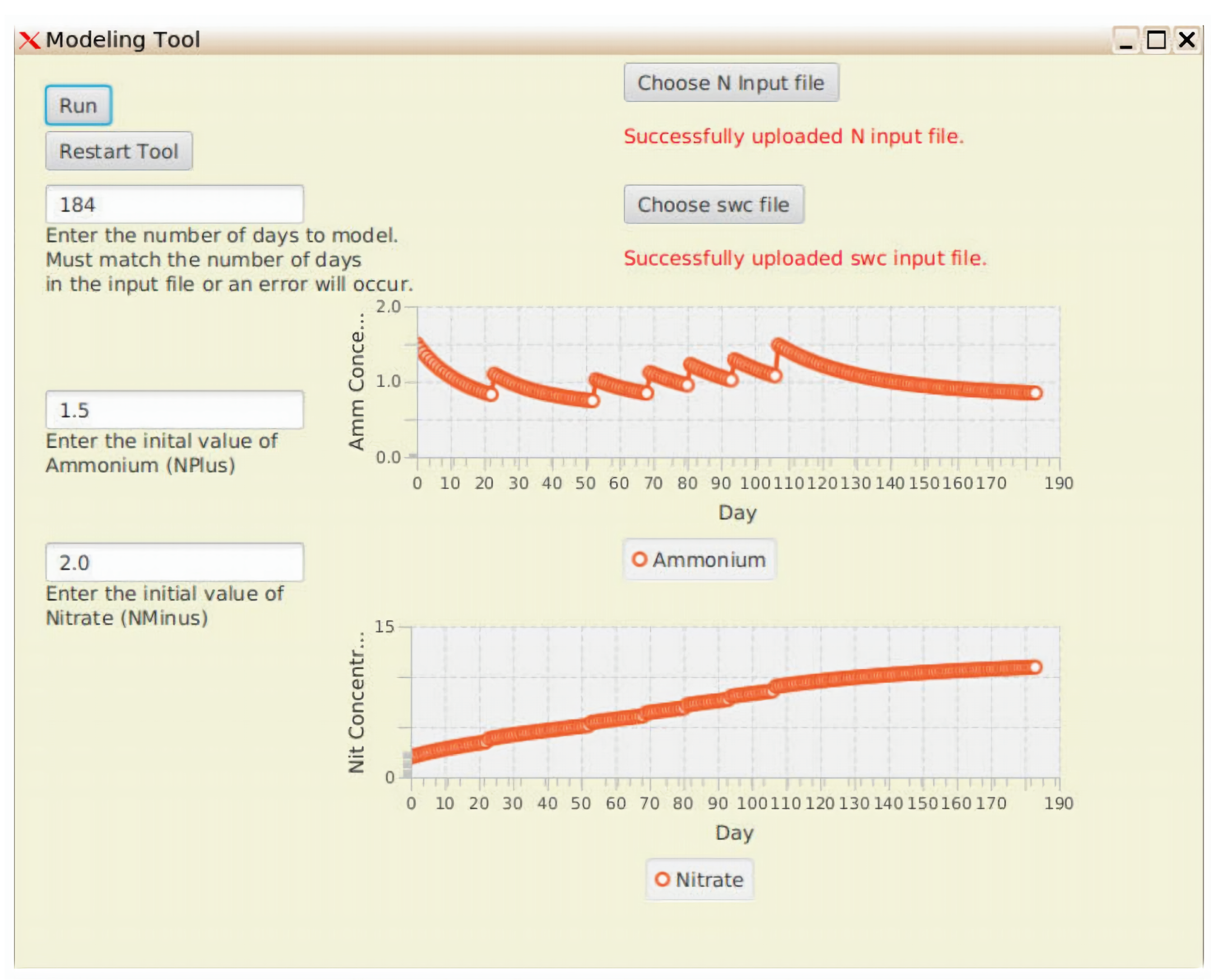
3.4.1. Hosting of Lean N-Model in MyGeoHub

Our implementation of the lean N-model [10] is hosted in MyGeoHub. To host any tool in MyGeoHub, an account has to be created and approved by the administration team at MyGeoHub. User specific files can be stored in it much like Google Drive. To create a tool, one has to navigate to Contribute under the Resources drop-down menu on Account home page. When creating the tool, details like Tool name, ID, and description are to be given, which we did. After this step, SVN (Apache Subversion, subversion.apache.org) repository, an open source version control system, similar to a simple version of Git, was set up. The SVN software was downloaded on the local computer and synced to the tool being developed on MyGeoHub. Doing this allows a tool developer to add files to a filesystem on a local development machine, which can then be committed to the SVN server. MyGeoHub then uses the code in the SVN server to deploy the tool in it.

The lean N-model [10] was implemented in Java programming language using the JavaFX library. JavaFX is an extensive Java library that supports the creation of complete applications and user interfaces that supports user input and output using JavaFX buttons, text input boxes, file upload buttons, and graphs. Several validations and error displays were put into place for the input; for example, non-negativity of ammonium and nitrate values, proper format of ammonium, nitrate and soil moisture file.

The makefile for our tool compiled the source code, used the generated class files to create a jar executable file, and then moved the executable file to the bin directory. The makefile was tricky to format because it runs commands in the command line, and the local development computer runs windows while the MyGeoHub platform runs Linux. Windows and Linux use different commands in the command line and also may have different versions of Java installed, so a makefile that works on a local computer would likely fail when run on the MyGeoHub platform. With guidance from the support team of MyGeoHub to figure out what commands to use, Virtual Linux machines were used to test the makefile commands that worked in MyGeoHub as well. Hence, it is advisable to develop the tool in a local development computer that is also running on a Linux operating system. Another issue that needed to be resolved is that file upload buttons in the tool would open the files of the MyGeoHub Linux machine instead of the files on the tool users’ local machine, making file uploading from the users’ local machine impossible. This was resolved by adding a line to the invoke file that enabled a special MyGeoHub file uploading tool. This enabled any tool user to use this uploading tool to upload their files to the MyGeoHub Linux system and then use the uploading buttons on the tool to choose their files from the Linux machine.

The lean N-model is deployed at https://mygeohub.org/tools/benfeddersen (accessed on 28 March 2021). Any user with a MyGeoHub account can access the tool. The tool inputs daily soil moisture values and daily nitrate and ammonia prescriptions to the soil. After launching the tool, the input files have to be uploaded from user’s local computer to the MyGeoHub user space using the MyGeoHub file upload tool, as shown in Figure 7. Number of days for simulation, initial nitrate, and ammonium values are to be entered through the input boxes shown in Figure 8. Then nitrate, ammonium, and soil moisture input files have to be provided by clicking on the buttons (named Choose N input file and Choose swc file) shown in Figure 8. The file input buttons in Figure 8 choose files from the MyGeoHub user space. One can run the tool by clicking the Run button in the top left corner. The tool would then generate and display two graphs, as shown in Figure 8. One can also click the Restart button to clear the graphs and restart the tool. Note if the tool is restarted, the step mentioned in Figure 7 can be skipped because the files will still be uploaded to the Linux machine.

4. Results

Following the general framework of Figure 5, we set the benchmark model to be RZWQM, and the test model is taken to be the lean N-model of [10]. The benchmark model calibration algorithm used is coordinated descent from our prior work [37,76]. The coordinated descent method showed good model prediction of the field data, with a coefficient of determination ($R^2$) of 0.79. The field data (1) is taken from USDA experimental field in Greeley, CO [66], which consists of soil moisture and plant growth. The parameters calibrated in the RZWQM model are eight hydraulics at seven depths and three crop growth parameters (total 59). The outputs (6) and (11) compared are daily nitrate and ammonium outputs. The output data of calibrated RZWQM in (6) was used to calibrate 12 parameters (9) of the lean N test model using Particle Swarm Optimization (7). The calibrated lean N-model (10) is run with the parameters in (9) to output daily nitrate and ammonia values (11). The outputs from (6) and (11) are compared in (12) visually through plots and quantitatively using the coefficient of determination.

For the calibrated RZWQM, we examined its daily nitrate and ammonia predictions (under no crop) and used those values to calibrate our lean N-model [10], implemented in Python and JavaFX (and hosted in MyGeoHub run). Its nutrient parameters, namely, $a^{+},a^{-},b,K_S,r_h,r_r,k_d,k_l,k_h,k_n,k_i^{+},k_i^{+}$ were calibrated against the RZWQM predicted (as a substitute for field N data) nitrate and ammonia data.

The lean N-model parameter calibration was done using PSO (Particle Swarm Optimization [77]) in Python. PSO is a stochastic technique inspired by social behavior of bird flocking in search of food. PSO is initialized with a group of random particles (candidate solutions). It searches for the optimum by updating through iterations. In every iteration each particle’s velocity and position is updated by following two best values. First is the position of the best solution the particle itself has achieved so far. Second is the best solution attained so far by any particle in the swarm. pyswarm library in Python was used to implement the PSO algorithm, which also has the constraint optimization capability. The constraints imposed by us were the lower and upper range of the nutrient parameters so that physically practical values fit the data.

The lower and upper range and calibrated values obtained by PSO are summarized in Table 2. The population size of the PSO used was 100,000, and the PSO algorithm terminated in about 1000 iterations when its cost function could not be reduced further. We fitted both nitrate and ammonia values by defining the cost function for the PSO as the sum of weighted RMSE of ammonia and nitrate. The weights used were the inverse mean of the RZWQM predicted values of ammonia and nitrate, respectively. (This is because, while nitrate and ammonia use the same units, numerical values for nitrate is much higher than those of ammonia.) The RMSE upon termination was found to be 0.8353.

The plot of ammonia and nitrate values from two different models is given below in Figure 9 and Figure 10, respectively. The plots show similar predictions by the two models, with the figure of merit of the fit as measured by the coefficient of determination ($R^2$) to be 0.99 and 0.62 (1 being a perfect fit) for nitrate and ammonia, respectively. In addition, while a run of RZWQM takes 12 s without the SHAW module and 70 s with that SHAW module, the runtime for the lean N-model is only 0.35 s. However, it should be remarked that RZWQM must also simulate the soil water and heat modules, apart from the N-cycle module. The lean model is thus also more flexible. Time required by PSO to calibrate the lean N-model was 1.5 h.

5. Discussion

Figure 9 and Figure 10 show promising results. The occurrences of the peaks and the rates of rise and fall are comparable. Some mismatch is understandable as the lean model does not assume many physical processes and works with lesser nitrogen pools. RZWQM also discretizes the soil into many layers (with different soil properties if required), which is avoided in the lean model. We can conclude that the lean N-model with fewer pools and parameters yields reasonably accurate ammonium and nitrate plots, helpful for faster prototyping. We attribute the possible reason of ammonia data having the fitting value of $R^2$ = 0.62 (as compared to nitrate data having a fit value of $R^2$ = 0.99) to the lean N-model not accounting for ammonia volatilization (loss of soil ammonium to atmosphere as ammonia gas). The volatilization process is implemented in RZWQM, and it depends on wind speed, soil temperature, and the partial pressure gradient of ammonia.

The lean N-model is easier to implement, calibrate (online and offline), and faster. High dimension optimization has a very large search space, and exploring it with a model with long execution time is not practical. In this regard, the lean N-model facilitates a quick initial phase of global optimization, whereas a complex model can later be used to fine-tune the optimization, starting from the output of the initial lean model based optimization.

To host and serve the model and related tools within the cloud, MyGeoHub was chosen. Hosting it there required some learning and support from their team. However, after that, managing and configuration creation, like setting up server, database, and sessions, are all taken care of by MyGeoHub.

The unavailability of high frequency field nutrient data is due to the unavailability of in-situ soil sensors. However, with recent advances in portable in-situ soil moisture, nutrient, and gas sensors, including the ones from our research group [78,79,80,81,82], there is a great possibility of high frequency measurement of soil and plant variables, which can then be used to calibrate the models independent of each other.

6. Conclusions

A general framework for model comparison when field data may limit direct comparison of models is proposed, developed, and also demonstrated. The framework first calibrates the benchmark model against the field data, and next it calibrates the test model against the data generated by the calibrated benchmark model. Using the proposed framework, this work qualitatively compared popular N models based on their modeling complexity and quantitatively compared a most complex one (RZWQM) with the least complex one (a lean N-model) to understand the gap and possibility of using a lean model for the sake of fast prototyping. In addition, to the best of our knowledge, there is no literature comparing the N-model of RZWQM with the lean model by Porporato et al. [10] with respect to the field data of Greeley, CO. Our prior calibration work [37] improved upon the then state-of-art calibration of RZWQM against Greeley, CO, field data performed by an agriculture expert [67]. Here we used [37] to calibrate RZWQM and used its simulated data to then calibrate the lean N-model. The models were then compared visually through plots as well as quantitatively through the coefficient of determination.

We implemented in Python a lean reliable alternative for a soil nutrient dynamics module, calibrated it using particle swarm optimizer also written in Python, and compared the prediction results of the model with the state-of-art complex model, RZWQM. The lean N-model showed good prediction accuracy vis-a-vis RZWQM, providing $R^2$ model accuracy of 0.99 and 0.62 for nitrate and ammonia, respectively, and afforded speed-up over RZWQM in runtime. Having a lean, accurate model enables fast prototyping of offline designs. The implemented lean N-model was hosted in MyGeoHub to be universally accessible to the community. Development and integration of lean water flow and crop growth modules are possible future extensions. Accordingly, in the long term, we envision integrating most agriculture processes, automated model calibration, and optimized decision recommender in one platform, one that would be independent of a user operating system and accessible anywhere through the internet.

References

1. Jones, J.W.; Antle, J.M.; Basso, B.; Boote, K.J.; Conant, R.T.; Foster, I.; Godfray, H.C.J.; Herrero, M.; Howitt, R.E.; Janssen, S.; et al. Brief history of agricultural systems modeling. Agric. Syst. 2017, 155, 240–254. [Google Scholar] [CrossRef]
2. De Wit, C.T. Transpiration and Crop Yields; Technical Report; WILEY: Hoboken, NJ, USA, 1958. [Google Scholar]
3. Van Bavel, C. A Drought Criterion and Its Application in Evaluating Drought Incidence and Hazard 1. Agron. J. 1953, 45, 167–172. [Google Scholar] [CrossRef]
4. Shaffer, M.J.; Pierce, F.J. A user’s guide to NTRM, a soil-crop simulation model for nitrogen, tillage, and crop-residue management. In Conservation Research Report (USA); U.S. Dept. of Agriculture, Agricultural Research Service: Washington, DC, USA, 1987. [Google Scholar]
5. Shaffer, M.; Halvorson, A.; Pierce, F. Nitrate leaching and economic analysis package (NLEAP): Model description and application. In Managing Nitrogen for Groundwater Quality and Farm Profitability; Soil Science Soc Amer: Madison, WI, USA, 1991; pp. 285–322. [Google Scholar]
6. Molina, J.; Clapp, C.; Shaffer, M.; Chichester, F.; Larson, W. NCSOIL, a model of nitrogen and carbon transformations in soil: Description, calibration, and behavior. Soil Sci. Soc. Am. J. 1983, 47, 85–91. [Google Scholar] [CrossRef]
7. Parton, W. The CENTURY model. In Evaluation of Soil Organic Matter Models; Springer: Berlin/Heidelberg, Germany, 1996; pp. 283–291. [Google Scholar]
8. Parton, W.J.; Hartman, M.; Ojima, D.; Schimel, D. DAYCENT and its land surface submodel: Description and testing. Glob. Planet. Chang. 1998, 19, 35–48. [Google Scholar] [CrossRef]
9. Hansen, S.; Jensen, H.; Shaffer, M. Developments in modeling nitrogen transformations in soil. In Nitrogen Fertilization in the Environment; Marcel Dekker: New York, NY, USA, 1995; pp. 83–107. [Google Scholar]
10. Porporato, A.; D’odorico, P.; Laio, F.; Rodriguez-Iturbe, I. Hydrologic controls on soil carbon and nitrogen cycles. I. Modeling scheme. Adv. Water Resour. 2003, 26, 45–58. [Google Scholar] [CrossRef]
11. Jones, J.W.; Hoogenboom, G.; Porter, C.H.; Boote, K.J.; Batchelor, W.D.; Hunt, L.; Wilkens, P.W.; Singh, U.; Gijsman, A.J.; Ritchie, J.T. The DSSAT cropping system model. Eur. J. Agron. 2003, 18, 235–265. [Google Scholar] [CrossRef]
12. Dzotsi, K.; Jones, J.; Adiku, S.; Naab, J.; Singh, U.; Porter, C.; Gijsman, A. Modeling soil and plant phosphorus within DSSAT. Ecol. Model. 2010, 221, 2839–2849. [Google Scholar] [CrossRef]
13. Sharpley, A.N.; Williams, J.R. EPIC-Erosion/Productivity Impact Calculator. I: Model Documentation. II: User Manual. In Technical Bulletin-United States Department of Agriculture; US Department of Agriculture: Washington, DC, USA, 1990. [Google Scholar]
14. Jones, C.; Cole, C.; Sharpley, A.; Williams, J. A simplified soil and plant phosphorus model: I. Documentation. Soil Sci. Soc. Am. J. 1984, 48, 800–805. [Google Scholar] [CrossRef]
15. Williams, J.; Izaurralde, R.; Steglich, E. Agricultural policy/environmental extender model. Theor. Doc. Version 2008, 604, 2008–2017. [Google Scholar]
16. Taiz, L.; Zeiger, E.; Møller, I.M.; Murphy, A. Plant Physiology and Development; Sinauer Associates Incorporated: Sunderland, MA, USA, 2015. [Google Scholar]
17. Thornley, J.H.; France, J. Mathematical Models in Agriculture: Quantitative Methods for the Plant, Animal and Ecological Sciences; CABI: Wallingford, UK, 2007. [Google Scholar]
18. Williams, J.; Jones, C.; Kiniry, J.; Spanel, D.A. The EPIC crop growth model. Trans. ASAE 1989, 32, 497–0511. [Google Scholar] [CrossRef]
19. Ritchie, J. Description and performance of CERES wheat: A user-oriented wheat yield model. In ARS Wheat Yield Project; USDA-ARS: Ames, IA, USA, 1985; pp. 159–175. [Google Scholar]
20. Van Diepen, C.v.; Wolf, J.; Van Keulen, H.; Rappoldt, C. WOFOST: A simulation model of crop production. Soil Use Manag. 1989, 5, 16–24. [Google Scholar] [CrossRef]
21. SimUnek, J.; Van Genuchten, M.T.; Sejna, M. The HYDRUS Software Package for Simulating the Two-And Three-Dimensional Movement of Water, Heat, and Multiple Solutes in Variably-Saturated Porous Media. In Technical Manual; 2012; Available online: www.researchgate.net/ (accessed on 31 January 2021).
22. Radcliffe, D.E.; Simunek, J. Soil Physics with HYDRUS: Modeling and Applications; CRC Press: Boca Raton, FL, USA, 2018. [Google Scholar]
23. Douglas-Mankin, K.; Srinivasan, R.; Arnold, J. Soil and Water Assessment Tool (SWAT) model: Current developments and applications. Trans. ASABE 2010, 53, 1423–1431. [Google Scholar] [CrossRef]
24. Gassman, P.W.; Reyes, M.R.; Green, C.H.; Arnold, J.G. The soil and water assessment tool: Historical development, applications, and future research directions. Trans. ASABE 2007, 50, 1211–1250. [Google Scholar] [CrossRef] [Green Version]
25. Saxton, K.E.; Willey, P.H. The SPAW model for agricultural field and pond hydrologic simulation. In Watershed Models; CRC Press: Boca Raton, FL, USA, 2005; pp. 400–435. [Google Scholar]
26. Van Dam, J.C.; Huygen, J.; Wesseling, J.; Feddes, R.; Kabat, P.; Van Walsum, P.; Groenendijk, P.; Van Diepen, C. Theory of SWAP Version 2.0; Simulation of Water Flow, Solute Transport and Plant Growth in the Soil-Water-Atmosphere-Plant Environment; Technical Report; DLO Winand Staring Centre: Wageningen, The Netherlands, 1997. [Google Scholar]
27. Holzworth, D.P.; Huth, N.I.; de Voil, P.G.; Zurcher, E.J.; Herrmann, N.I.; McLean, G.; Chenu, K.; van Oosterom, E.J.; Snow, V.; Murphy, C.; et al. APSIM–evolution towards a new generation of agricultural systems simulation. Environ. Model. Softw. 2014, 62, 327–350. [Google Scholar] [CrossRef]
28. Keating, B.A.; Carberry, P.S.; Hammer, G.L.; Probert, M.E.; Robertson, M.J.; Holzworth, D.; Huth, N.I.; Hargreaves, J.N.; Meinke, H.; Hochman, Z.; et al. An overview of APSIM, a model designed for farming systems simulation. Eur. J. Agron. 2003, 18, 267–288. [Google Scholar] [CrossRef] [Green Version]
29. Stockle, C.O.; Martin, S.A.; Campbell, G.S. CropSyst, a cropping systems simulation model: Water/nitrogen budgets and crop yield. Agric. Syst. 1994, 46, 335–359. [Google Scholar] [CrossRef]
30. Stöckle, C.O.; Donatelli, M.; Nelson, R. CropSyst, a cropping systems simulation model. Eur. J. Agron. 2003, 18, 289–307. [Google Scholar] [CrossRef]
31. Ahuja, L.; Rojas, K.; Hanson, J. Root Zone Water Quality Model: Modelling Management Effects on Water Quality and Crop Production; Water Resources Publication: Highlands Ranch, CO, USA, 2000. [Google Scholar]
32. Zhang, Y.; Li, C.; Zhou, X.; Moore, B., III. A simulation model linking crop growth and soil biogeochemistry for sustainable agriculture. Ecol. Model. 2002, 151, 75–108. [Google Scholar] [CrossRef]
33. Thorp, K.; Youssef, M.; Jaynes, D.; Malone, R.; Ma, L. DRAINMOD-N II: Evaluated for an agricultural system in Iowa and compared to RZWQM-DSSAT. Trans. ASABE 2009, 52, 1557–1573. [Google Scholar] [CrossRef]
34. Kozak, J.A.; Aiken, R.M.; Flerchinger, G.N.; Nielsen, D.C.; Ma, L.; Ahuja, L. Comparison of modeling approaches to quantify residue architecture effects on soil temperature and water. Soil Tillage Res. 2007, 95, 84–96. [Google Scholar] [CrossRef]
35. Wiborg, T. A Comparison of Agricultural Sector Models: CRAM, DRAM, SASM and the KVL Model; Technical Report; 2000; Available online: https://ageconsearch.umn.edu/record/24211/files/ew000002.pdf (accessed on 28 March 2021).
36. Parajuli, P.B.; Nelson, N.O.; Frees, L.D.; Mankin, K.R. Comparison of AnnAGNPS and SWAT model simulation results in USDA-CEAP agricultural watersheds in south-central Kansas. Hydrol. Process. Int. J. 2009, 23, 748–763. [Google Scholar] [CrossRef]
37. Bhar, A.; Kumar, R.; Qi, Z.; Malone, R. Coordinate descent based agricultural model calibration and optimized input management. Comput. Electron. Agric. 2020, 172, 105353. [Google Scholar] [CrossRef]
38. Bhar, A.; Kumar, R. Model-Predictive Real-Time Fertilization and Irrigation Decision-Making Using RZWQM. In Proceedings of the 2019 ASABE Annual International Meeting. American Society of Agricultural and Biological Engineers, Boston, MA, USA, 7–10 July 2019; p. 1. [Google Scholar]
39. Kalyanam, R.; Zhao, L.; Song, C.; Biehl, L.; Kearney, D.; Kim, I.L.; Shin, J.; Villoria, N.; Merwade, V. MyGeoHub—A sustainable and evolving geospatial science gateway. Future Gener. Comput. Syst. 2019, 94, 820–832. [Google Scholar] [CrossRef]
40. McLennan, M.; Kennell, R. HUBzero: A platform for dissemination and collaboration in computational science and engineering. Comput. Sci. Eng. 2010, 12, 48–53. [Google Scholar] [CrossRef]
41. Wu, L.; McGechan, M.; McRoberts, N.; Baddeley, J.; Watson, C. SPACSYS: Integration of a 3D root architecture component to carbon, nitrogen and water cycling—Model description. Ecol. Model. 2007, 200, 343–359. [Google Scholar] [CrossRef]
42. Sadhukhan, D.; Qi, Z.; Zhang, T.; Tan, C.S.; Ma, L.; Andales, A.A. Development and evaluation of a phosphorus (P) module in RZWQM2 for phosphorus management in agricultural fields. Environ. Model. Softw. 2019, 113, 48–58. [Google Scholar] [CrossRef]
43. Hansen, S.; Jensen, H.; Nielsen, N.; Svendsen, H. DAISY: Soil plant atmosphere system model. NPO Rep. A 1990, 10, 272. [Google Scholar]
44. Liang, H.; Hu, K.; Batchelor, W.D.; Qi, Z.; Li, B. An integrated soil-crop system model for water and nitrogen management in North China. Sci. Rep. 2016, 6, 25755. [Google Scholar] [CrossRef] [Green Version]
45. Jansson, P.E. CoupModel: Model use, calibration, and validation. Trans. ASABE 2012, 55, 1337–1344. [Google Scholar] [CrossRef]
46. Smith, J.; Gottschalk, P.; Bellarby, J.; Chapman, S.; Lilly, A.; Towers, W.; Bell, J.; Coleman, K.; Nayak, D.; Richards, M.; et al. Estimating changes in Scottish soil carbon stocks using ECOSSE. I. Model description and uncertainties. Clim. Res. 2010, 45, 179–192. [Google Scholar] [CrossRef] [Green Version]
47. Gerik, T.; Williams, J.; Francis, L.; Greiner, J.; Magre, M.; Meinardus, A.; Steglich, E.; Taylor, R. Environmental Policy Integrated Climate Model-User’s Manual Version 0810; Blackland Research and Extension Center; Texas A&M AgriLife: Temple, TX, USA, 2014. [Google Scholar]
48. Parton, B.; Ojima, D.; Del Grosso, S.; Keough, C. CENTURY Tutorial: Supplement to CENTURY User’s Manual. In Great Plain System Research Unit Technical Report; 2001; Available online: https://www2.nrel.colostate.edu/projects/century/century_tutorial.pdf (accessed on 28 March 2021).
49. Li, C.; Frolking, S.; Frolking, T.A. A model of nitrous oxide evolution from soil driven by rainfall events: 1. Model structure and sensitivity. J. Geophys. Res. Atmos. 1992, 97, 9759–9776. [Google Scholar] [CrossRef]
50. Johnsson, H.; Bergstrom, L.; Jansson, P.E.; Paustian, K. Simulated nitrogen dynamics and losses in a layered agricultural soil. Agric. Ecosyst. Environ. 1987, 18, 333–356. [Google Scholar] [CrossRef]
51. Williams, J.R.; Izaurralde, R.; Singh, V.; Frevert, D. The APEX model. In Watershed Models; CRC Press: Boca Raton, FL, USA, 2006; pp. 437–482. [Google Scholar]
52. Li, Y.; White, R.; Chen, D.; Zhang, J.; Li, B.; Zhang, Y.; Huang, Y.; Edis, R. A spatially referenced water and nitrogen management model (WNMM) for (irrigated) intensive cropping systems in the North China Plain. Ecol. Model. 2007, 203, 395–423. [Google Scholar] [CrossRef]
53. Kersebaum, K.C. Application of a simple management model to simulate water and nitrogen dynamics. Ecol. Model. 1995, 81, 145–156. [Google Scholar] [CrossRef]
54. Nendel, C. MONICA: A simulation model for nitrogen and carbon dynamics in agro-ecosystems. In Novel Measurement and Assessment Tools for Monitoring and Management of Land and Water Resources in Agricultural Landscapes of Central Asia; Springer: Berlin/Heidelberg, Germany, 2014; pp. 389–405. [Google Scholar]
55. Kersebaum, K.C. Modelling nitrogen dynamics in soil–crop systems with HERMES. In Modelling Water and Nutrient Dynamics in Soil–Crop Systems; Springer: Berlin/Heidelberg, Germany, 2007; pp. 147–160. [Google Scholar]
56. Franko, U.; Oelschlägel, B.; Schenk, S. Simulation of temperature-, water-and nitrogen dynamics using the model CANDY. Ecol. Model. 1995, 81, 213–222. [Google Scholar] [CrossRef]
57. Franko, U.; Oelschlägel, B.; Schenk, S.; Puhlmann, M.; Kuka, K.; Mallast, J.; Thiel, E.; Prays, N.; Meurer, K.; Bönecke, E. CANDY Manual—Description of Background; UFZ; Halle: Leipzig, Germany, 2015. [Google Scholar]
58. De Willigen, P. Nitrogen turnover in the soil-crop system; comparison of fourteen simulation models. In Nitrogen Turnover in the Soil-Crop System; Springer: Berlin/Heidelberg, Germany, 1991; pp. 141–149. [Google Scholar]
59. De Willigen, P.; Neeteson, J. Comparison of six simulation models for the nitrogen cycle in the soil. Fertil. Res. 1985, 8, 157–171. [Google Scholar] [CrossRef]
60. Wu, L.; McGechan, M. A review of carbon and nitrogen processes in four soil nitrogen dynamics models. J. Agric. Eng. Res. 1998, 69, 279–305. [Google Scholar] [CrossRef]
61. Manzoni, S.; Porporato, A. Soil carbon and nitrogen mineralization: Theory and models across scales. Soil Biol. Biochem. 2009, 41, 1355–1379. [Google Scholar] [CrossRef]
62. Shaffer, M.J.; Ma, L.; Hansen, S. Modeling Carbon and Nitrogen Dynamics for Soil Management; CRC Press: Boca Raton, FL, USA, 2001. [Google Scholar]
63. Dessureault-Rompré, J.; Zebarth, B.J.; Georgallas, A.; Burton, D.L.; Grant, C.A.; Drury, C.F. Temperature dependence of soil nitrogen mineralization rate: Comparison of mathematical models, reference temperatures and origin of the soils. Geoderma 2010, 157, 97–108. [Google Scholar] [CrossRef]
64. Rodrigo, A.; Recous, S.; Neel, C.; Mary, B. Modelling temperature and moisture effects on C–N transformations in soils: Comparison of nine models. Ecol. Model. 1997, 102, 325–339. [Google Scholar] [CrossRef]
65. Antonopoulos, V.Z. Comparison of different models to simulate soil temperature and moisture effects on nitrogen mineralization in the soil. J. Plant Nutr. Soil Sci. 1999, 162, 667–675. [Google Scholar] [CrossRef]
66. Trout, T.J.; Bausch, W.C. USDA-ARS Colorado maize water productivity data set. Irrig. Sci. 2017, 35, 241–249. [Google Scholar] [CrossRef]
67. Qi, Z.; Ma, L.; Bausch, W.C.; Trout, T.J.; Ahuja, L.R.; Flerchinger, G.N.; Fang, Q. Simulating maize production, water and surface energy balance, canopy temperature, and water stress under full and deficit irrigation. Trans. ASABE 2016, 59, 623–633. [Google Scholar]
68. Wilkins-Diehr, N.; Gannon, D.; Klimeck, G.; Oster, S.; Pamidighantam, S. TeraGrid science gateways and their impact on science. Computer 2008, 41, 32–41. [Google Scholar] [CrossRef]
69. Wang, S.; Liu, Y. TeraGrid GIScience gateway: Bridging cyberinfrastructure and GIScience. Int. J. Geogr. Inf. Sci. 2009, 23, 631–656. [Google Scholar] [CrossRef]
70. Klimeck, G.; McLennan, M.; Brophy, S.P.; Adams, G.B., III; Lundstrom, M.S. nanohub. org: Advancing education and research in nanotechnology. Comput. Sci. Eng. 2008, 10, 17. [Google Scholar] [CrossRef]
71. Allison, J.; Backman, D.; Christodoulou, L. Integrated computational materials engineering: A new paradigm for the global materials profession. Jom 2006, 58, 25–27. [Google Scholar] [CrossRef]
72. Goff, S.A.; Vaughn, M.; McKay, S.; Lyons, E.; Stapleton, A.E.; Gessler, D.; Matasci, N.; Wang, L.; Hanlon, M.; Lenards, A.; et al. The iPlant collaborative: Cyberinfrastructure for plant biology. Front. Plant Sci. 2011, 2, 34. [Google Scholar] [CrossRef] [Green Version]
73. CIF21 DIBBs: PD: Cyberinfrastructure Tools for Precision Agriculture in the 21st Century. Available online: https://www.nsf.gov/awardsearch/showAward?AWD_ID=1724843 (accessed on 28 March 2021).
74. Tarboton, D.G.; Idaszak, R.; Ames, D.; Goodall, J.; Horsburgh, J.; Band, L.; Merwade, V.; Song, C.; Couch, A.; Valentine, D.; et al. HydroShare: An Online, Collaborative Environment for the Sharing of Hydrologic Data and Models; 2012; Available online: https://digitalcommons.usu.edu/cgi/viewcontent.cgi?article=3691&context=cee_facpub (accessed on 28 March 2021).
75. Rosenzweig, C.; Jones, J.W.; Hatfield, J.L.; Ruane, A.C.; Boote, K.J.; Thorburn, P.; Antle, J.M.; Nelson, G.C.; Porter, C.; Janssen, S.; et al. The agricultural model intercomparison and improvement project (AgMIP): Protocols and pilot studies. Agric. For. Meteorol. 2013, 170, 166–182. [Google Scholar] [CrossRef] [Green Version]
76. Bhar, A.; Qi, Z.; Malone, R.W.; Kumar, R. Sensor data driven parameter estimation for Agricultural Model using Coordinate Descent. In Proceedings of the 2018 ASABE Annual International Meeting, American Society of Agricultural and Biological Engineers, Detroit, MI, USA, 29 July–1 August 2018; p. 1. [Google Scholar]
77. Kennedy, J.; Eberhart, R. Particle swarm optimization. Proceedings of ICNN’95-International Conference on Neural Networks, Perth, WA, Australia, 27 November–1 December 1995; IEEE: New York, NY, USA, 1995; Volume 4, pp. 1942–1948. [Google Scholar]
78. Xu, Z.; Wang, X.; Weber, R.J.; Kumar, R.; Dong, L. Nutrient sensing using chip scale electrophoresis and in situ soil solution extraction. IEEE Sens. J. 2017, 17, 4330–4339. [Google Scholar] [CrossRef]
79. Pandey, G.; Kumar, R.; Weber, R.J. A low RF-band impedance spectroscopy based sensor for in situ, wireless soil sensing. IEEE Sens. J. 2014, 14, 1997–2005. [Google Scholar] [CrossRef]
80. Pandey, G.; Weber, R.J.; Kumar, R. Agricultural cyber-physical system: In-situ soil moisture and salinity estimation by dielectric mixing. IEEE Access 2018, 6, 43179–43191. [Google Scholar] [CrossRef]
81. Kashyap, B.; Kumar, R. Sensing Methodologies in Agriculture for Soil Moisture and Nutrient Monitoring. IEEE Access 2021, 9, 14095–14121. [Google Scholar] [CrossRef]
82. Tabassum, S.; Kumar, R.; Dong, L. Nanopatterned optical fiber tip for guided mode resonance and application to gas sensing. IEEE Sens. J. 2017, 17, 7262–7272. [Google Scholar] [CrossRef]
Figure 1. Generic nitrogen cycle in agriculture setting [9].
Inventions 06 00025 g001
Figure 2. Various Carbon pools of the lean soil nutrient dynamics model [10].
Inventions 06 00025 g002
Figure 3. Various Nitrogen pools of the lean soil nutrient dynamics model [10].
Inventions 06 00025 g003
Figure 4. Variation of soil moisture factor with relative soil moisture [10].
Inventions 06 00025 g004
Figure 5. Generic setup for model comparison.
Inventions 06 00025 g005
Figure 6. MyGeoHub Hubzero infrastructures; adapted from [39].
Inventions 06 00025 g006
Figure 7. Screen grab of file upload window in MyGeoHub. (Left): Tool window to upload and download files between local computer and MyGeoHub user space. (Right): File browser to choose a local file to be uploaded to MyGeoHub.
Inventions 06 00025 g007
Figure 8. MyGeoHub implementation interface and displays.
Inventions 06 00025 g008
Figure 9. Plot of ammonia concentration by two models for each day of year of the growing season.
Inventions 06 00025 g009
Figure 10. Plot of nitrate concentration by two models for each day of year of the growing season.
Inventions 06 00025 g010