Article

Autonomous Mobile Ground Control Point Improves Accuracy of Agricultural Remote Sensing through Collaboration with UAV

1
Department of Biological and Agricultural Engineering, Texas A&M University, College Station, TX 77843, USA
2
Department of Biosystems Engineering, College of Agriculture and Life Sciences, Kangwon National University, Chuncheon, Kangwon 24341, Korea
*
Author to whom correspondence should be addressed.
Inventions 2020, 5(1), 12; https://doi.org/10.3390/inventions5010012
Submission received: 31 October 2019 / Revised: 22 January 2020 / Accepted: 25 January 2020 / Published: 2 March 2020
(This article belongs to the Special Issue Robotics and Automation in Agriculture)

Abstract

:
Ground control points (GCPs) are critical for agricultural remote sensing that require georeferencing and calibration of images collected from an unmanned aerial vehicles (UAV) at different times. However, the conventional stationary GCPs are time-consuming and labor-intensive to measure, distribute, and collect their information in a large field setup. An autonomous mobile GCP and a collaboration strategy to communicate with the UAV were developed to improve the efficiency and accuracy of the UAV-based data collection process. Prior to actual field testing, preliminary tests were conducted using the system to show the capability of automatic path tracking by reducing the root mean square error (RMSE) for lateral deviation from 34.3 cm to 15.6 cm based on the proposed look-ahead tracking method. The tests also indicated the feasibility of moving reflectance reference panels successively along all the waypoints without having detrimental effects on pixel values in the mosaicked images, with the percentage errors in digital number values ranging from −1.1% to 0.1%. In the actual field testing, the autonomous mobile GCP was able to successfully cooperate with the UAV in real-time without any interruption, showing superior performances for georeferencing, radiometric calibration, height calibration, and temperature calibration, compared to the conventional calibration method that has stationary GCPs.

1. Introduction

The use of unmanned aerial vehicles (UAVs) as platforms to collect high-resolution multi-spectral imagery is increasing rapidly in a wide variety of environmental and geographical studies including in agriculture [1,2,3], forestry [4,5,6], ecology [7,8,9], mining [10,11,12], coastal assessments [13,14,15], and fluvial surveys [16,17,18]. In agriculture, obtaining the accurate and timely status of crop growth, such as canopy greenness, leaf area, water stress estimation, and various geographic features, including crop area and digital surface models (DSMs), especially measured systematically over the growing season, is of great interest to plant breeders and agronomists. Since UAV platforms can significantly improve the spatial and temporal resolution of field images, they are increasingly used in precision agriculture to maximize crop yield and to protect crops from losses [19,20]. To accelerate breeding and genetics research, many types of imaging sensors, such as RGB [21,22], multispectral [23,24], and thermal [25,26], are used on UAVs for mapping phenotypes at the plot or plant scale resolution [27,28,29]. The increasing capabilities of such remote sensing techniques are continuously pushing boundaries in agronomy and plant science, leading to the development of efficient management practices and selection of superior plant varieties to meet current and future food demand.
Ground control points (GCPs) are used in creating aerial image mosaics, and their helpfulness depends on their quality and quantity. Most UAVs are equipped with low-quality global positioning system (GPS) receivers that are used to record the camera position during image capture, with a few exceptions that use high-accuracy GPS [30,31,32]. Thus, employing high-precision GCPs in field survey measurements is generally critical to improve the geometric accuracy and quality of digital terrain models (DTMs), DSMs, and image mosaics [33,34]. In addition, some studies [35,36,37] have demonstrated that increasing the quantity of GCPs installed across the fields, especially when the area of interest is large, can remarkably improve photogrammetric surveys.
Precision agriculture is aimed at optimizing farming by maximizing productivity while minimizing costs [38] and environmental risks. It depends on sensing technologies to provide spatiotemporal field data for accurate positioning and mapping, data-analysis techniques for multivariate optimization of mapped data, and automation technologies to apply the right types and amounts of production inputs at optimal times and locations. Wireless networks have recently been introduced in precision agriculture to gather and transmit field data [39]. In a non-mobile wireless network architecture, the networked devices (nodes) are at fixed positions; e.g., in irrigation management, water quality monitoring [40,41], control of humidity, temperature, carbon dioxide, and other significant factors in greenhouses [42,43]. In a mobile architecture, the node devices move across the field during operational periods; e.g., with data collection by farm vehicles, when a central farm manager or computer oversees farm operations [44]. Numerous studies have demonstrated the utility of wireless network technology in precision agriculture, but most have been limited to specific limited applications over short distances. In one of our recent studies [45], a system of multifunctional GCPs and a wireless network to communicate with the UAV were developed to improve the speed of GCP setup and provide GCP data collection in real-time during UAV flights. The GCPs used in this study were not conventional single-purpose systems. They demonstrated excellent potential for georeferencing, radiometric, and height calibrations to reduce remote-sensing errors, and automating real-time communication to maximize efficiency.
Collaboration among multiple autonomous vehicles could improve work rates and allow time-critical tasks to meet deadlines by scaling up the number of operational machines [46,47]. Collaboration occurs when multiple vehicles share the same general task at the same time, and it requires real-time wireless communication among vehicles on a peer-to-peer basis [48]. There has been widespread interest in the investigation of collaborative motion control of fleets of autonomous vehicles in agriculture [49].
One application in which collaboration may be particularly useful is in-field calibration of remote-sensing systems. True calibration requires not simply sensor calibration, but measuring a known object in the environment where unknown objects will be measured. Sensor values from the unknown objects are then adjusted relative to the measurements of the known object. To be repeatable from location to location and date to date, UAV measurements of plant reflectance, height, and temperature require radiometric, height, and temperature calibrations. Radiometric calibration provides consistent reflectance data under a wide range of environmental conditions [50,51]. GCPs with known reflectance can be placed in the field, and crop reflectance data can be rapidly acquired by flying the UAV equipped with a camera. The data can then later be calibrated with respect to the GCPs’ reflectance in post-processing, or possibly in real-time. Vegetation indices from the calibrated data can potentially be used for making decisions and performing actions in farm management [52,53]. Height calibration involves improving the accuracy of crop height estimation based on the DSM. Known-height GCPs can be used to provide height calibration data [54]. During the growing season, variability in the height of crops provides essential information on plant health, growth, and response to environmental effects. Recent studies have shown that crop height can be derived from 3D dense point cloud data derived from structure-from-motion (SfM) [55,56], and GCP-based height calibration improves the accuracy of plant-height estimates [54]. Furthermore, UAV-based thermal remote sensing has been applied to agricultural purposes, including plant disease detection, irrigation scheduling, evaluation of fruit maturity, and detection of bruises in fruits and vegetables [57,58]. Using UAVs to acquire highly accurate thermal image data requires integration with thermal references on the ground. Ribeiro-Gomes et al. [59] proposed a calibration method for uncooled thermal cameras based on a neural network, considering the sensor temperature and the digital response of each pixel as input data. Thermal imaging has remained underexploited in the remote sensing domain for high throughput phenotyping [60,61]. During thermal radiometric calibration, accounting for environmental conditions that prevail during UAV image acquisition is very important for good accuracy [62,63]. Han et al. [64] demonstrated the feasibility of using thermoelectric module-based temperature-controlled reference panels for calibrating thermal images with reasonable accuracy in a wheat field. Carefully conducted data calibration is time-consuming and labor-intensive based on the current methods. Therefore, it is essential to develop automated calibration systems and methods that are appropriate for UAV-image data collection in agriculture.
The overall goal of this research was to develop an autonomous mobile GCP for accurate UAV-based agricultural remote sensing, in order to optimize the cost, productivity, efficiency, and environmental impacts associated with agricultural production. Specific objectives of this study were (1) to design, build, and test collaborative ground and aerial autonomous vehicles for acquisition of calibrated agricultural remote sensing data and (2) to evaluate the autonomous mobile GCP in terms of quality of georeferencing and calibration for reflectance, height, and temperature as compared to the conventional system with fixed GCPs.

2. Materials and Methods

2.1. Unmanned Mobile GCP

2.1.1. Structure

An autonomous mobile GCP (Figure 1) was constructed with aluminum structure to minimize weight while maintaining adequate strength. The GCP platform consists of a robotic base layer, a control-unit layer, and a reference layer. The base layer consists of two DC Brushless motors (10 inch-1000W; QS Motor, Taizhou, Zhejiang, China), two motor drivers (QSKBS48101X; QS Motor, Taizhou, Zhejiang, China), two motor batteries (48V-20Ah; QS Motor, Taizhou, Zhejiang, China), two rechargeable batteries (SLR155; Vmax, Belleville, MI, USA), and four spring-loaded caster wheels (eight inch, 200lb; Shepherd Hardware Products, Three Oaks, MI, USA). The design of the base layer enabled differential speed steering control of the front wheels in rugged agricultural terrains. The control-unit layer hosted the following: (1) a high-level controller with an industrial computer (ML500G-50; Logic Supply, South Burlington, VT, USA) that served as a navigation terminal to run path tracking algorithms; (2) two RTK-GPS units (C94-M8P RTK-GPS; Ublox, Thalwil, Switzerland) that enabled determination of positions and heading angles of the mobile GCP; (3) an XBee radio transceiver (XBP9B-DMST-002; Digi International, Minnetonka, MN, USA) for communication between the UAV and mobile GCP; (4) a low-level controller with a field-programmable gate array (FPGA) embedded processor (myRIO-1900; National Instrument, Austin, TX, USA) to operate the motor wheels; and (5) two temperature controllers (090097; Droking, Guangzhou, Guangdong, China) to control the thermal reference panels. Similar to the hardware setup used in our previous studies [64], the two prototype temperature calibration reference panels (cooling and heating) and the two radiometric calibration reference panels (dark gray and light gray) installed on the reference layer facilitated calibration of images from cameras, such as RGB, multispectral, and thermal.

2.1.2. Navigation System

The autonomous navigation of the GCP was based on a path tracking algorithm implemented through a control system consisting of high-level and low-level controllers (Figure 2). While the high-level controller regulated navigation, the low-level controller regulated differential speed steering. Navigation in the high-level control module was based on waypoint tracking principles: when the mobile GCP arrives within a pre-defined limit of boundary offset (LBO) distance of a waypoint, or deviates from the target path, the high-level controller tries to maintain trajectory by searching for the next waypoint. The waypoint data, created in the route data definition file (RDDF) format [65], were used for path planning commands that include waypoint indexes, northing and easting coordinates, LBO values, and traveling velocities. A look-ahead tracking method, which is conventionally used for autonomous navigation [66,67], was implemented to steer the mobile GCP on a trajectory defined by the pre-determined waypoints. Figure 3 depicts the look-ahead tracking method used to locate subsequent target points (e.g., point M ) on the path and determine corresponding steering angles, relative to the current position of the mobile GCP. For a path look-ahead distance ( L t ), defined as the length of the prospective path, an imaginary point A was determined by adding the look-ahead distance to the current location (point A ) in its direction of motion. Line A M , perpendicular to line A A , was constructed and the target point M was projected at the point of intersection of line A M and line W P n   W P n + 1 . For each generated target point, the steering angle of the mobile GCP was re-calculated to guide the system along the path based on the look-ahead tracking method. The steering angle at each location was calculated by subtracting the new waypoint angle ( θ 1 ) from the heading angle ( θ 2 ).
The real-time corrections for steering angle and velocity were relayed from the high-level controller to the low-level controller through a universal asynchronous receiver/transmitter (UART) serial communication device. The differential steering required to change the orientation of the GCP and make it turn was achieved by unbalancing the left and right motor voltages, which resulted in one drive running faster than the other to make a more gradual turn, rather than an in-place turn that rotates about a central point. The difference in rotational speeds was proportional to the magnitude and direction of the steering angle and was controlled by a closed-loop motor speed controller that used speed values measured from the rotary encoders of the motor wheel as feedback signals.

2.2. Unmanned Aerial Systems

A quadcopter UAV (Matrice 100; DJI, Shenzhen, Guangdong, China) was used to collect remote-sensing data and, in collaboration with the autonomous mobile GCP, enable calibration. The UAV was autonomously piloted with mission planning software (Pix4Dcapture; Pix4D SA, Lausanne, Switzerland) and remotely controlled during flights with DJI’s remote controller. The maximum flight time was approximately 20 min, with a maximum range of 2 km and a maximum take-off weight of 3.6 kg. Prior to field testing, a multispectral camera (RedEdge; MicaSense, Seattle, WA, USA) installed on the UAV was used in a preliminary test; then an RGB camera (Zenmuse X3; DJI, Shenzhen, Guangdong, China) and a thermal camera (ICI 8640 P-series; Infrared Cameras Inc; Beaumont, TX, USA) were carried on the UAV separately to investigate whether the proposed autonomous mobile GCP would perform as expected for collaborative remote-sensing calibration. All the cameras were triggered by an onboard controller to vary the frame rate based on flight speed for optimal overlap between images.
The UAV was equipped with a modified RTK-GPS system (Figure 4) consisting of a low-cost GPS module (C94-M8P RTK-GPS; Ublox, Thalwil, Switzerland), an Arduino controller (UNO; Arduino, Somerville, MA, USA), a STM32 microcontroller (STM32F103C8T6; STMicroelectronics, Geneva, Switzerland), and separate XBee radio receiver and transmitter units (XBP9B-DMST-002; Digi International, Minnetonka, MN, USA). An RTK base station was used and included an Ublox GPS module serving in base mode, a STM32 microcontroller, and an Xbee radio transmitter unit. The differential-correction signals from the base station were transmitted through the XBee radio receiver to the STM32 microcontroller mounted on the UAV, which then delivered the signals to the GPS-rover module through the UART serial communication interface to achieve high GPS accuracy (within 2 cm error) in real-time. The corrected coordinates of the UAV during the flight were transmitted to the autonomous mobile GCP at 10 Hz with a baud rate of 19,200 bps through the Arduino controller and the XBee radio transmitter.

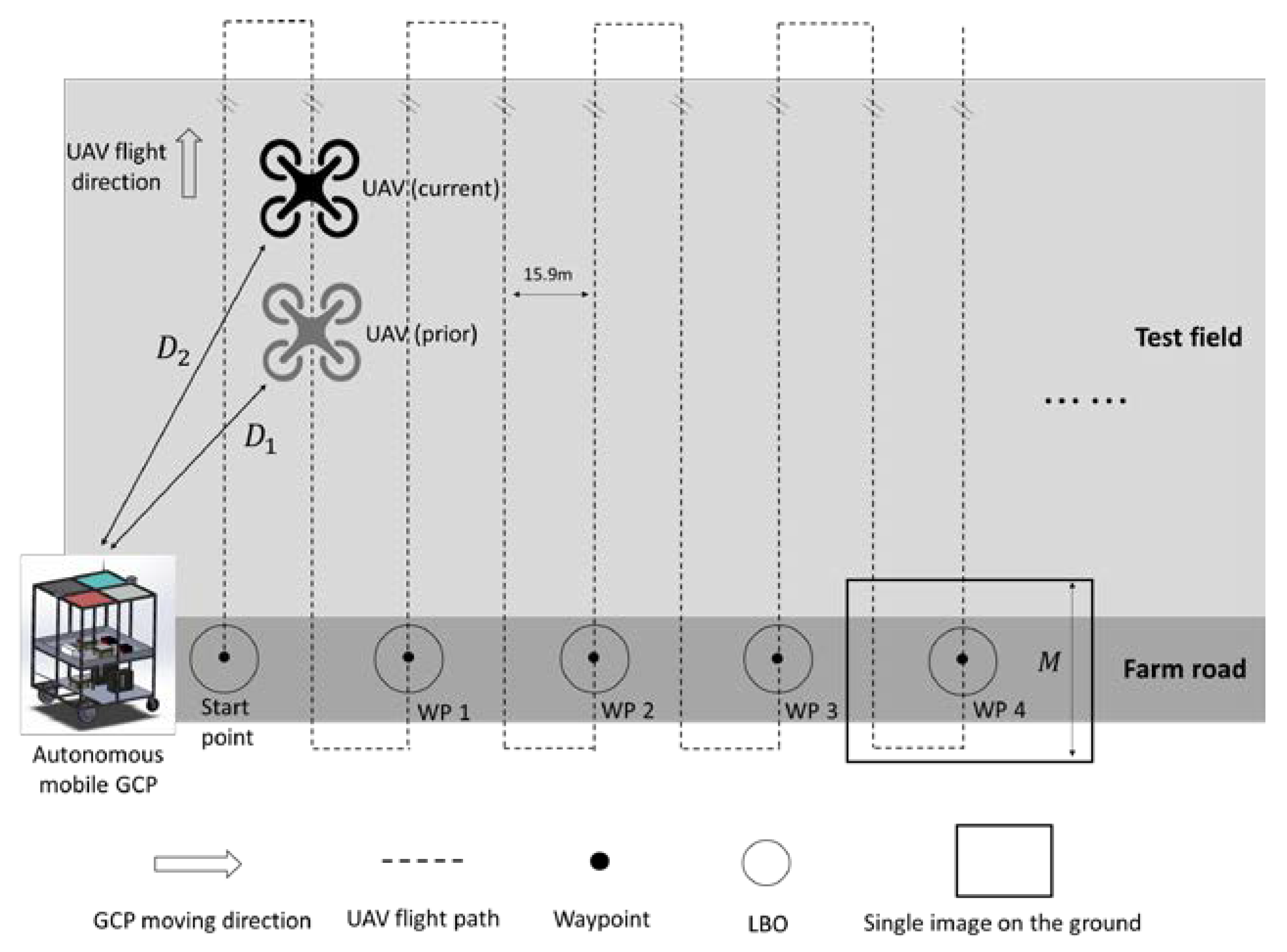
2.3. Collaboration Strategy

The autonomous mobile GCP has the potential to replace multiple conventional fixed GCPs [45,54], which have been used to improve the quality of image data and increase the efficiency of the calibration process. A collaboration strategy was proposed as shown in Figure 5. The mobile GCP was first placed close to the UAV starting point, and it subsequently navigated to the LBO of the starting point during takeoff. The decision to move towards the next target point was made based on the UAV coordinates sent continuously to the mobile GCP. The GCP control system checked whether the distance between the two platforms ( D ) exceeded a threshold value ( M ), which is the width of the ground footprint captured in the aerial imagery. The decision to move also depended on the direction of flight away from the mobile GCP, which was determined by checking whether the distance between subsequent points in the direction of flight increased continually ( D 1 < D 2 ). If all conditions were met, it was assumed the mobile GCP had been imaged by the UAV at the waypoint, and then the next waypoint should be used as a new target point. The mobile GCP reached the target point before the UAV returned and approached the mobile GCP within the threshold range M . The process was to be repeated in a cyclical manner throughout the flight.

2.4. Experimental Design

2.4.1. Preliminary Tests

Two preliminary tests were conducted with the autonomous mobile GCP. Prior to conducting field tests, the autonomous tracking was tested on flat ground to investigate whether the mobile GCP would follow a pre-defined path, and also to evaluate its performance in autonomous maneuvering. An RDDF was created for a predefined path with a U-turn that connected two 25-m long parallel paths. The trajectories of the mobile GCP as it traveled at 3 km/h were recorded to compare two path-tracking algorithms: simple waypoint tracking and look-ahead tracking. The second part of preliminary testing was to investigate the appropriate moving distance of the mobile GCP to improve UAV remote sensing data. The UAV was flown with the multispectral camera at an altitude of 60 m above ground level (AGL) and a ground speed of approximately 15 m/s. Two 61-cm square reflectance reference panels (dark gray and light gray) were manually moved along the field road with two movement patterns during UAV flights. The panels were first placed on successive waypoints, and second on only odd-numbered successive waypoints, after the UAV had flown away from the previous waypoint (Figure 5). The distances between two adjacent flight paths were 15.9 m, and the size of a single image on the ground (i.e., black-color rectangle) was 53 m × 49 m. To investigate the effects of the GCP movement on image quality in each mosaicked image, the digital numbers (DNs) extracted from the reflectance references on the mosaicked images were compared to the raw images, which included the corresponding reflectance reference panels.

2.4.2. Field Tests

The experiment was conducted within two hours of solar noon in a 0.1 km2 cotton field at the Texas A&M AgriLife research farm (headquarters at latitude 30.549635 N, longitude 96.436821 W in the WGS-84 coordinate system) near College Station, Texas, USA (Figure 6). Two UAV flights, with RGB and thermal cameras flown separately, were conducted at 45 m AGL with ground speed of roughly 17 m/s, to achieve approximate ground resolutions of 1.93 cm and 6.62 cm during the respective flights. A 75% overlap in both forward and sideward directions was achieved for both the RGB and thermal images. Mosaicking of the RGB and thermal images was performed with Pix4Dmapper (Pix4D SA, Lausanne, Switzerland) software. Two image-processing methods (conventional and a proposed new method) were implemented with ArcMap 10.3 (ESRI, Redlands, CA, USA) to evaluate the effectiveness of the autonomous mobile GCP for georeferencing, radiometric calibration, height calibration, and temperature calibration.
Conventional calibration was implemented by georeferencing the image mosaic with coordinates from the RTK-GPS system on four fixed GCPs that had been developed in our previous research [54]. These were installed semi-permanently on the ground at the corners of the test field. Consistent with the method used in our previous study, height calibration of the DSM was performed by fitting three points, extracted from the upper and lower levels of a multi-level GCP and the ground, into a linear equation. This fixed GCP, fastened to the ground on the southwest side of the field, had three 61-cm square calibration reference panels (dark, medium, and light gray) installed at both levels. Radiometric calibration of the image mosaic was implemented with a linear equation derived by fitting the average DN values to reflectance values of the calibration reference panels in each spectral band. To calibrate temperature with the conventional method, the average DN values of the fixed color panels on the multi-level GCP were extracted, and then calibration parameters were calculated by using temperatures measured with an IR thermometer (Fluke 64 MAX, Fluke, Everett, WA, USA).
The proposed calibration method involved using the mobile GCP in autonomous operation to follow a predefined path, which included six waypoints along the farm road on the southwest side of the test field. The strategy for collaboration between GCP and UAV, which was used to determine the state of the mobile GCP at each waypoint, was based on the positions of the UAV during flight. The spatial coordinates measured aboard the mobile GCP at each stopping point were used for georeferencing, and the height and reference panel reflectance values at each of these points were used for calibration. Height calibration was performed by fitting a linear equation through known height values of the ground and the reference layer of the mobile GCP. Radiometric calibration was performed based on reflectance from the dark and light gray reference panels mounted on top of the mobile GCP. To perform temperature calibration of the thermal image mosaic, the temperature reference panels installed on the top of the mobile GCP were powered on in advance for 10 min to ensure stable temperatures before UAV-based thermal image collection. The temperature control modules were set to 20 °C for the low-temperature reference and 60 °C for the high-temperature reference, to cover the full range of temperature variations that crops experience during the season. Consistent with the method used in our previous study [64], temperature calibration of the image mosaic was performed with a linear calibration equation based on pixel values extracted from the low-temperature reference and high-temperature reference. These values were the median of all pixels arranged on each temperature reference.
Accuracies of measurements obtained from the UAV-based images from the conventional and the proposed autonomous mobile GCP-based calibration methods were evaluated for georeferencing and object reflectance, height, and temperature calibrations in the image mosaic. To validate radiometric calibration, the average reflectance error for each band in the calibrated image mosaic was calculated from reflectance values of three differently colored panels (dark, medium, and light gray), which were placed on the southwest and northeast sides of the test field. Similar to the test for radiometric calibration, the average height error in the calibrated DSM was calculated based on two different heights of boxes (54.6 cm and 109.2 cm) placed near the differently colored panels. Georeferencing accuracy was validated by comparing horizontal accuracies of center point coordinates on the four boxes, as estimated from the calibrated image mosaic, with the actual coordinates measured with the RTK-GPS. The surface temperatures of the color panels extracted from the calibrated thermal image mosaic were compared with the manual temperature measurements taken around the time of UAV flight with the Fluke IR thermometer.

3. Results and Discussion

3.1. Preliminary Tests

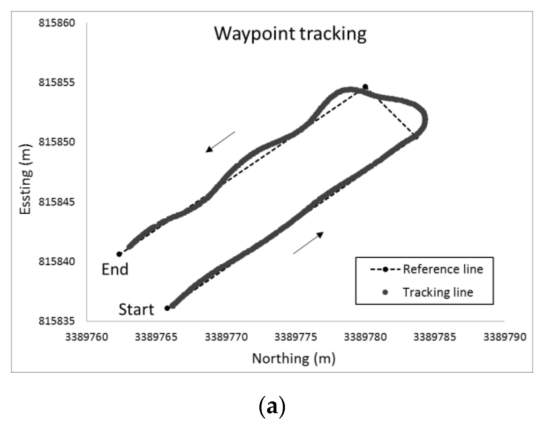
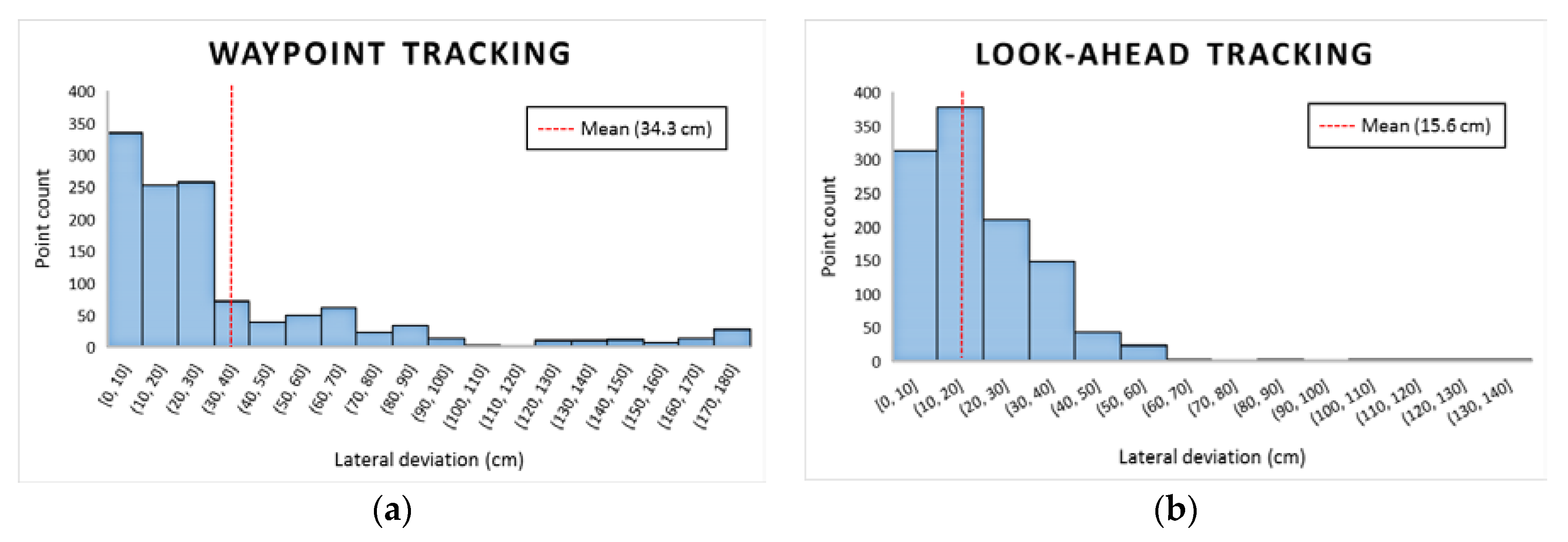
3.1.1. Evaluation of Path Tracking Accuracy

Figure 7a,b show the actual trajectories of the mobile GCP along a U-shaped path on asphalt pavement, obtained from the simple waypoint tracking and the look-ahead tracking methods, respectively. There was little difference in the trajectories between the two methods on the first straight path. However, the efficiency of look-ahead tracking became evident along the turn and the second straight path, as the mobile GCP was more stable and maintained its trajectory along the predefined path. Look-ahead tracking had a root mean square error (RMSE) in tracking that remained within an acceptable range of 20 cm along the two straight paths. In contrast, simple waypoint tracking had a much larger RMSE (Table 1). Figure 8 presents the histograms of the lateral deviations along the entire trajectory for the two tracking methods. Most of the sampling points were distributed between 0 and 20 cm for the look-ahead tracking method, with the average error in deviation being 15.6 cm. In summary, the preliminary test showed that the look-ahead tracking method performed better in path tracking and, hence, it is a better candidate for autonomous navigation of the mobile GCP for UAV remote sensing.

3.1.2. Difference of DNs Error between Image Mosaic and Single Image

Figure 9a,b show portions of the mosaicked image obtained when the two reflectance reference panels were moved along the farm road for every waypoint in the flight path and every odd numbered waypoints in the flight path, respectively. When the reflectance reference panels were compared between the two image mosaics, no apparent difference was observed. The average DN values of the reflectance reference panels from single images were compared with DN values from the mosaicked images. When the reflectance panels were moved to each waypoint (Figure 10a), the percentage differences between mosaicked and raw images were low (−1.1–0.1%). When the panels were moved only to the odd numbered waypoints (Figure 10b), the errors were −4.2–1.3%. Moving the mobile GCP to each waypoint reduced the errors possibly because having more proximal references better captured spatial variability in the field, and having more tie points during mosaicking improved the image quality and, hence, the reflectance accuracy. This preliminary test also showed that there should be no significant concern about errors that might result from moving reflectance reference panels during flights, an advance over current agricultural UAV remote-sensing research, which typically uses stationary reflectance reference panels in the field.

3.2. Field Tests

3.2.1. Collaboration between UAV and Mobile GCP

Figure 11a shows the actual trajectories of the UAV (black dots) and the autonomous mobile GCP (yellow dots) that were synchronized with the collaboration strategy mentioned previously. The mobile GCP operated autonomously, without any interruption, and traversed to predefined waypoints with a maximum lateral deviation <15 cm (RMSE = 5.8 cm). Figure 11b shows the results of heading angles and operation mode commands obtained from the mobile GCP along the farm road. There was no change in heading angle when the mobile GCP was stopped at each waypoint, and heading fluctuated from 297.3° to 317.3° when in motion. Overall the mobile GCP performed as expected, stopping or moving forward along the six waypoints when the operation commands changed from on (“1”) to off (“0”) or from off to on, respectively. The proposed path tracking algorithm and collaboration strategy worked effectively to establish communication between the UAV and the mobile GCP.

3.2.2. Evaluating the Accuracy of Image Calibration

Table 2 compares the errors in georeferencing, radiometric calibration, height calibration, and temperature calibration for the conventional and proposed methods. The coordinates of the boxes placed in the field (Figure 6), extracted from the two image mosaics, indicated that our proposed method has better georeferencing accuracy: within 10 cm of the coordinates measured with the RTK-GPS. Although the proposed method significantly reduced georeferencing errors on the southwest side of the field where the mobile GCP platform traversed, there was no noticeable improvement on the northeast side of the field farther from the mobile GCP. This result indicates the potential of the proposed method for including more GCPs to cover regions of the field too far away to benefit from a single mobile GCP.
The proposed method also performed better in terms of radiometric calibration, with error in calibration ranging from 0.115% to 2.771%, as compared to 1.364–6.556% for the conventional method. These results indicate that radiometric calibration based on the mobile GCP can more efficiently account for variation in illumination and atmospheric conditions on UAV images taken across the field, compared to those obtained with only one set of calibration panels.
The linear height calibration of the proposed method reduced errors in object height estimation (<4 cm) on both sides of the field, compared to the height estimation errors (<6 cm) that resulted from the conventional method. One point to note, however, is that shorter boxes had relatively high height estimation errors. This is consistent with the results observed in other studies [68,69] where point clouds of shorter objects and crops had higher estimation errors. Due to their proximity to the ground and relatively low pixel representation, shorter objects produce fewer image gradients to effectively distinguish them from ground pixels during SfM reconstruction. This suggests that mounting reference panels on taller mobile GCPs can improve the calibration accuracy in height estimation.
Linear calibrations for temperature in both the conventional and the proposed methods significantly improved the correlation between the ground truth measurements and the mean temperature extracted from the calibrated image pixels that corresponded to the three different color panels. Actual temperatures ranged from 43.4 °C to 52.2 °C. As expected, the proposed method had smaller errors in temperature estimation (2.0 °C–3.26 °C) due to the accurately controlled temperature reference panels on the mobile GCP, compared to the conventional method (3.4 °C–7.6 °C). This reduction in error has important implications and shows potential for the proposed method to be used for various applications, including monitoring of crop stresses, crop diseases, and soil water stress, and planning for irrigation scheduling and harvesting operations. The main advantage of the mobile GCP is that it has a specific and tight dynamic temperature range from 20 °C to 60 °C to cover temperature variations in crops, as opposed to the conventional method, which only can calibrate over a narrow range of high temperatures (41 °C–54 °C) during the summer season. More accurate temperature measurements based on the proposed method can improve on-farm decision-making. In summary, the results from the field tests validated the potential of an autonomous mobile GCP in accurate georeferencing, radiometric calibration, height calibration, and temperature calibration of UAV-based agricultural remote sensing data.

3.3. Benefits, Challenges, and Future Work

The mobile GCP proposed in this project can be beneficial in terms of both cost and technical efficiency for a range of agricultural studies, including precision management and high throughput phenotyping. The design, which was based on low-cost mechanical and electronic components, cost approximately $3600 in total. However, labor cost was not accounted for since the system was developed in the lab. As discussed in the previous sections, using a mobile GCP synchronized with the flight pattern of the UAV can reduce the time and labor involved in deploying multiple GCPs across the field, while simultaneously providing better outcomes in terms of accuracies in parameter calibration and estimation.
Some of the practical limitations that were observed with the mobile GCP during the course of the project were (1) low stability while navigating through uneven terrains due to heavy-weight of the system and low capability of suspensions, (2) maintaining stable temperatures on the cooling panel during hot summer days with the current setup, and (3) lack of coverage in parts of the field farther away from the mobile GCP’s path, which resulted in un-uniform accuracies in parameter estimation across the field. The future work will focus on overcoming the above-mentioned limitations by (1) improving the structural design of the mobile GCP in terms of stability and ruggedness, (2) attaching additional cooling units for stable cooling panel temperature, and (3) using two or more mobile GCPs based on other cooperation strategies in order to obtain more uniform coverage for accurate calibration and estimation. Additionally, we will also focus on the optimization of waypoints in order to improve the overlap between images and adapt to fields with irregular boundaries. A possible source of error in UAV remote-sensing data is camera auto exposure, which changes the exposure-time and gain settings for each image, such that reflectance values are not collected consistently across a field. For this reason, efforts are needed to enable UAV-based cameras to use consistent optimal settings throughout the flight mission.

4. Conclusions

An autonomous mobile GCP was developed for the purposes of improving UAV-based agricultural data collection efficiency and georeferencing, radiometric, height, and temperature calibration accuracies. A navigation system was developed for automatic path tracking and wireless communication between the autonomous GCP and UAV for collaboration in field operations. Look-ahead tracking (RMSE = 15.6 cm) was superior to simple waypoint tracking (RMSE = 34.3 cm) for path tracking and proved to be an excellent candidate for autonomous navigation. Moving the mobile GCP along every waypoint in the flight path gave low percentage errors (−1.1–0.1%) in radiometric calibration compared to moving along only the odd-numbered waypoints. Lastly, errors in georeferencing and radiometric, height, and temperature calibrations from the proposed mobile-GCP method were significantly lower compared to those obtained from the conventional method. Overall these results indicate that the collaboration strategy between the autonomous mobile GCP and the UAV has potential to improve accuracy and efficiency in agricultural remote sensing applications. In the future fixed exposure with the multispectral camera can be used to reduce errors in reflectance estimation [70], and more validation objects be employed to more strongly demonstrate the reliability of using autonomous mobile GCPs for agricultural remote sensing.

Author Contributions

Conceptualization: X.H. and J.A.T.; Methodology: X.H. and J.A.T.; Software: X.H. and T.W.; Validation: X.H. and V.S.; Formal analysis: X.H.; Investigation: X.H.; Resources: T.W. and V.S.; Data curation: X.H. and J.A.T.; Writing—original draft preparation: X.H.; Writing—review and editing: J.A.T., V.S. and T.W.; Supervision: J.A.T.; Funding acquisition: J.A.T. All authors have read and agreed to the published version of the manuscript.

Funding

This work was funded by Texas A&M AgriLife Research, the United Sorghum Checkoff Program–Expansion of AgriLife Research TERRA Activities to Grain Sorghum (no. CI016-16), and USDA NIFA–Enhancing Accessibility, Reliability, and Validation of Actionable Information from the UAV-Image Data (no. 191000.321646.01).

Acknowledgments

The authors would like to express their sincere gratitude to the anonymous reviewers for their very useful and valuable comments that helped significantly in improving the quality of this paper.

Conflicts of Interest

The authors declare no conflict of interest.

References

  1. Han, L.; Yang, G.; Dai, H.; Xu, B.; Yang, H.; Feng, H.; Li, Z.; Yang, X. Modeling maize above-ground biomass based on machine learning approaches using UAV remote-sensing data. Plant Methods 2019, 15, 10. [Google Scholar] [CrossRef] [PubMed] [Green Version]
  2. Shi, Y.; Thomasson, J.A.; Murray, S.C.; Pugh, N.A.; Rooney, W.L.; Shafian, S.; Rajan, N.; Rouze, G.; Morgan, C.L.; Neely, H.L. Unmanned aerial vehicles for high-throughput phenotyping and agronomic research. PLoS ONE 2016, 11, e0159781. [Google Scholar] [CrossRef] [PubMed] [Green Version]
  3. Zhang, L.; Zhang, H.; Niu, Y.; Han, W. Mapping Maize Water Stress Based on UAV Multispectral Remote Sensing. Remote Sens. 2019, 11, 605. [Google Scholar] [CrossRef] [Green Version]
  4. Näsi, R.; Honkavaara, E.; Blomqvist, M.; Lyytikäinen-Saarenmaa, P.; Hakala, T.; Viljanen, N.; Kantola, T.; Holopainen, M. Remote sensing of bark beetle damage in urban forests at individual tree level using a novel hyperspectral camera from UAV and aircraft. Urban For. Urban Green. 2018, 30, 72–83. [Google Scholar] [CrossRef]
  5. Park, J.Y.; Muller-Landau, H.C.; Lichstein, J.W.; Rifai, S.W.; Dandois, J.P.; Bohlman, S.A. Quantifying leaf phenology of individual trees and species in a tropical forest using unmanned aerial vehicle (UAV) images. Remote Sens. 2019, 11, 1534. [Google Scholar] [CrossRef] [Green Version]
  6. Leduc, M.B.; Knudby, A. Mapping wild leek through the forest canopy using a UAV. Remote Sens. 2018, 10, 70. [Google Scholar] [CrossRef] [Green Version]
  7. Ventura, D.; Bonifazi, A.; Gravina, M.; Belluscio, A.; Ardizzone, G. Mapping and classification of ecologically sensitive marine habitats using unmanned aerial vehicle (UAV) imagery and object-based image analysis (OBIA). Remote Sens. 2018, 10, 1331. [Google Scholar] [CrossRef] [Green Version]
  8. Díaz-Delgado, R.; Cazacu, C.; Adamescu, M. Rapid assessment of ecological integrity for LTER wetland sites by using UAV multispectral mapping. Drones 2019, 3, 3. [Google Scholar] [CrossRef] [Green Version]
  9. Arroyo-Mora, J.P.; Kalacska, M.; Inamdar, D.; Soffer, R.; Lucanus, O.; Gorman, J.; Naprstek, T.; Schaaf, E.S.; Ifimov, G.; Elmer, K.; et al. Implementation of a UAV–hyperspectral pushbroom imager for ecological monitoring. Drones 2019, 3, 12. [Google Scholar] [CrossRef] [Green Version]
  10. Ren, H.; Zhao, Y.; Xiao, W.; Hu, Z. A review of UAV monitoring in mining areas: Current status and future perspectives. Int. J. Coal. Sci. Technol. 2019, 6, 320–333. [Google Scholar] [CrossRef] [Green Version]
  11. Moudrý, V.; Urban, R.; Štroner, M.; Komárek, J.; Brouček, J.; Prošek, J. Comparison of a commercial and home-assembled fixed-wing UAV for terrain mapping of a post-mining site under leaf-off conditions. Int. J. Remote Sens. 2019, 40, 555–572. [Google Scholar] [CrossRef]
  12. Lee, S.; Choi, Y. Reviews of unmanned aerial vehicle (drone) technology trends and its applications in the mining industry. Geosyst. Eng. 2016, 19, 197–204. [Google Scholar] [CrossRef]
  13. Gonçalves, J.A.; Henriques, R. UAV photogrammetry for topographic monitoring of coastal areas. ISPRS J. Photogramm. 2015, 104, 101–111. [Google Scholar] [CrossRef]
  14. Balampanis, F.; Maza, I.; Ollero, A. Coastal areas division and coverage with multiple UAVs for remote sensing. Sensors 2017, 17, 808. [Google Scholar] [CrossRef] [PubMed]
  15. Laporte-Fauret, Q.; Marieu, V.; Castelle, B.; Michalet, R.; Bujan, S.; Rosebery, D. Low-Cost UAV for high-resolution and large-scale coastal dune change monitoring using photogrammetry. J. Mar. Sci. Eng. 2019, 7, 63. [Google Scholar] [CrossRef] [Green Version]
  16. Rhee, D.S.; Do Kim, Y.; Kang, B.; Kim, D. Applications of unmanned aerial vehicles in fluvial remote sensing: An overview of recent achievements. KSCE J. Civ. Eng. 2018, 22, 588–602. [Google Scholar] [CrossRef]
  17. Tamminga, A.D.; Eaton, B.C.; Hugenholtz, C.H. UAS-based remote sensing of fluvial change following an extreme flood event. Earth Surf. Proc. Land. 2015, 40, 1464–1476. [Google Scholar] [CrossRef]
  18. Carrivick, J.L.; Smith, M.W. Fluvial and aquatic applications of Structure from Motion photogrammetry and unmanned aerial vehicle/drone technology. Wiley Interdiscip. Rev. Water 2019, 6, e1328. [Google Scholar] [CrossRef] [Green Version]
  19. Salamí, E.; Barrado, C.; Pastor, E. UAV flight experiments applied to the remote sensing of vegetated areas. Remote Sens. 2014, 6, 11051–11081. [Google Scholar] [CrossRef] [Green Version]
  20. Zhang, C.; Kovacs, J.M. The application of small unmanned aerial systems for precision agriculture: A review. Precis. Agric. 2012, 13, 693–712. [Google Scholar] [CrossRef]
  21. Senthilnath, J.; Dokania, A.; Kandukuri, M.; Ramesh, K.N.; Anand, G.; Omkar, S.N. Detection of tomatoes using spectral-spatial methods in remotely sensed RGB images captured by UAV. Biosyst. Eng. 2016, 146, 16–32. [Google Scholar] [CrossRef]
  22. Kim, D.-W.; Yun, H.S.; Jeong, S.-J.; Kwon, Y.-S.; Kim, S.-G.; Lee, W.S.; Kim, H.-J. Modeling and testing of growth status for Chinese cabbage and white radish with UAV-based RGB imagery. Remote Sens. 2018, 10, 563. [Google Scholar] [CrossRef] [Green Version]
  23. Candiago, S.; Remondino, F.; De Giglio, M.; Dubbini, M.; Gattelli, M. Evaluating multispectral images and vegetation indices for precision farming applications from UAV images. Remote Sens. 2015, 7, 4026–4047. [Google Scholar] [CrossRef] [Green Version]
  24. Shi, X.; Han, W.; Zhao, T.; Tang, J. Decision support system for variable rate irrigation based on UAV multispectral remote sensing. Sensors 2019, 19, 2880. [Google Scholar] [CrossRef] [Green Version]
  25. Kelly, J.; Kljun, N.; Olsson, P.O.; Mihai, L.; Liljeblad, B.; Weslien, P.; Klemedtsson, L.; Eklundh, L. Challenges and best practices for deriving temperature data from an uncalibrated UAV thermal infrared camera. Remote Sens. 2019, 11, 567. [Google Scholar] [CrossRef] [Green Version]
  26. Araus, J.L.; Cairns, J.E. Field high-throughput phenotyping: The new crop breeding frontier. Trends Plant. Sci. 2014, 19, 52–61. [Google Scholar] [CrossRef]
  27. McCormick, R.F.; Truong, S.K.; Mullet, J.E. 3D sorghum reconstructions from depth images identify QTL regulating shoot architecture. Plant. Physiol. 2016, 172, 823–834. [Google Scholar] [CrossRef] [Green Version]
  28. Sodhi, P. In-Field Plant Phenotyping Using Model-Free and Model-Based Methods. Master’s Thesis, Carnegie Mellon University Pittsburgh, Pittsburgh, PA, USA, 2017. [Google Scholar]
  29. Batz, J.; Méndez-Dorado, M.A.; Thomasson, J.A. Imaging for high-throughput phenotyping in energy sorghum. J. Imaging 2016, 2, 4. [Google Scholar] [CrossRef]
  30. Turner, D.; Lucieer, A.; Wallace, L. Direct georeferencing of ultrahigh-resolution UAV imagery. IEEE Trans. Geosci. Remote Sens. 2014, 52, 2738–2745. [Google Scholar] [CrossRef]
  31. Eling, C.; Wieland, M.; Hess, C.; Klingbeil, L.; Kuhlmann, H. Development and evaluation of a UAV based mapping system for remote sensing and surveying applications. Int. Arch. Photogramm. Remote. Sens. Spat. Inf. Sci. 2015, 40, 233. [Google Scholar] [CrossRef] [Green Version]
  32. Mian, O.; Lutes, J.; Lipa, G.; Hutton, J.J.; Gavelle, E.; Borghini, S. Direct georeferencing on small unmanned aerial platforms for improved reliabiitily and accuracy of mapping without the need for ground control points. Int. Arch. Photogramm. Remote. Sens. Spat. Inf. Sci. 2015, 40, 397. [Google Scholar] [CrossRef] [Green Version]
  33. Wang, J.; Ge, Y.; Heuvelink, G.B.; Zhou, C.; Brus, D. Effect of the sampling design of ground control points on the geometric correction of remotely sensed imagery. Int. J. Appl. Earth Obs. 2012, 18, 91–100. [Google Scholar] [CrossRef]
  34. Hugenholtz, C.H.; Whitehead, K.; Brown, O.W.; Barchyn, T.E.; Moorman, B.J.; LeClair, A.; Riddell, K.; Hamilton, T. Geomorphological mapping with a small unmanned aircraft system (sUAS): Feature detection and accuracy assessment of a photogrammetrically-derived digital terrain model. Geomorphology 2013, 194, 16–24. [Google Scholar] [CrossRef] [Green Version]
  35. Gómez-Candón, D.; López-Granados, F.; Caballero-Novella, J.J.; Gómez-Casero, M.; Jurado-Expósito, M.; García-Torres, L. Geo-referencing remote images for precision agriculture using artificial terrestrial targets. Precis. Agric. 2011, 12, 876–891. [Google Scholar] [CrossRef] [Green Version]
  36. Agüera-Vega, F.; Carvajal-Ramírez, F.; Martínez-Carricondo, P. Assessment of photogrammetric mapping accuracy based on variation ground control points number using unmanned aerial vehicle. Measurement 2017, 98, 221–227. [Google Scholar] [CrossRef]
  37. Oniga, V.E.; Breaban, A.I.; Statescu, F. Determining the optimum number of ground control points for obtaining high precision results based on UAS images. Proceedings 2018, 2, 352. [Google Scholar] [CrossRef] [Green Version]
  38. Robert, P.C. Precision agriculture: A challenge for crop nutrition management. Plant. Soil 2002, 247, 143–149. [Google Scholar] [CrossRef]
  39. Sahota, H.; Kumar, R.; Kamal, A. A wireless sensor network for precision agriculture and its performance. Wirel. Commun. Mob. Comput. 2011, 11, 1628–1645. [Google Scholar] [CrossRef]
  40. Jiang, P.; Xia, H.; He, Z.; Wang, Z. Design of a water environment monitoring system based on wireless sensor networks. Sensors 2009, 9, 6411–6434. [Google Scholar] [CrossRef] [Green Version]
  41. Zhu, X.; Li, D.; He, D.; Wang, J.; Ma, D.; Li, F. A remote wireless system for water quality online monitoring in intensive fish culture. Comput. Electron. Agric. 2010, 71, S3–S9. [Google Scholar] [CrossRef]
  42. Hwang, J.; Shin, C.; Yoe, H. Study on an agricultural environment monitoring server system using wireless sensor networks. Sensors 2010, 10, 11189–11211. [Google Scholar] [CrossRef] [PubMed]
  43. Chaudhary, D.; Nayse, S.; Waghmare, L. Application of wireless sensor networks for greenhouse parameter control in precision agriculture. Int. J. Wirel. Mob. Netw. 2011, 3, 140–149. [Google Scholar] [CrossRef]
  44. Stentz, A.; Dima, C.; Wellington, C.; Herman, H.; Stager, D. A system for semi-autonomous tractor operations. Auton. Robot. 2002, 13, 87–104. [Google Scholar] [CrossRef]
  45. Han, X.; Thomasson, J.A.; Xiang, Y.; Gharakhani, H.; Yadav, P.K.; Rooney, W.L. Multifunctional ground control points with a wireless network for communication with a UAV. Sensors 2019, 19, 2852. [Google Scholar] [CrossRef] [PubMed] [Green Version]
  46. Noguchi, N.; Will, J.; Reid, J.; Zhang, Q. Development of a master–slave robot system for farm operations. Comput. Electron. Agric. 2004, 44, 1–19. [Google Scholar] [CrossRef]
  47. Johnson, D.A.; Naffin, D.J.; Puhalla, J.S.; Sanchez, J.; Wellington, C.K. Development and implementation of a team of robotic tractors for autonomous peat moss harvesting. J. Field Robot. 2009, 26, 549–571. [Google Scholar] [CrossRef] [Green Version]
  48. Blackmore, S.; Have, H.; Fountas, S. Specification of behavioural requirements for an autonomous tractor. In Proceedings of the American Society of Agricultural and Biological Engineers, Chicago, IL, USA, 26–27 July 2002; pp. 33–42. [Google Scholar]
  49. Emmi, L.; Gonzalez-de-Soto, M.; Pajares, G.; Gonzalez-de-Santos, P. New trends in robotics for agriculture: Integration and assessment of a real fleet of robots. Sci. World J. 2014, 2014, 21. [Google Scholar] [CrossRef] [Green Version]
  50. Cooley, T.; Anderson, G.P.; Felde, G.W.; Hoke, M.L.; Ratkowski, A.J.; Chetwynd, J.H.; Gardner, J.A.; Adler-Golden, S.M.; Matthew, M.W.; Berk, A.; et al. FLAASH, a MODTRAN4-based atmospheric correction algorithm, its application and validation. In Proceedings of the IEEE International Geoscience and Remote Sensing Symposium, Toronto, ON, Canada, 24–28 June 2002; pp. 1414–1418. [Google Scholar]
  51. Iqbal, F.; Lucieer, A.; Barry, K. Simplified radiometric calibration for UAS-mounted multispectral sensor. Eur. J. Remote Sens. 2018, 51, 301–313. [Google Scholar] [CrossRef]
  52. Yang, G.; Liu, J.; Zhao, C.; Li, Z.; Huang, Y.; Yu, H.; Xu, B.; Yang, X.; Zhu, D.; Zhang, X. Unmanned aerial vehicle remote sensing for field-based crop phenotyping: Current status and perspectives. Front. Plant. Sci. 2017, 8, 1111. [Google Scholar] [CrossRef]
  53. Tagle Casapia, M.X. Study of Radiometric Variations in Unmanned Aerial Vehicle Remote Sensing Imagery for Vegetation Mapping. Master’s Thesis, Lund University, Lund, Sweden, 2017. [Google Scholar]
  54. Han, X.; Thomasson, J.A.; Bagnall, G.C.; Pugh, N.A.; Horne, D.W.; Rooney, W.L.; Jung, J.; Chang, A.; Malambo, L.; Popescu, S.C.; et al. Measurement and calibration of plant-height from fixed-wing UAV images. Sensors 2018, 18, 4092. [Google Scholar] [CrossRef] [Green Version]
  55. Geipel, J.; Link, J.; Claupein, W. Combined spectral and spatial modeling of corn yield based on aerial images and crop surface models acquired with an unmanned aircraft system. Remote Sens. 2014, 6, 10335–10355. [Google Scholar] [CrossRef] [Green Version]
  56. Madec, S.; Baret, F.; De Solan, B.; Thomas, S.; Dutartre, D.; Jezequel, S.; Hemmerlé, M.; Colombeau, G.; Comar, A. High-throughput phenotyping of plant height: Comparing unmanned aerial vehicles and ground lidar estimates. Front. Plant. Sci. 2017, 8, 2002. [Google Scholar] [CrossRef] [PubMed] [Green Version]
  57. Ishimwe, R.; Abutaleb, K.; Ahmed, F. Applications of thermal imaging in agriculture—A review. Adv. Remote Sens. 2014, 3, 128. [Google Scholar] [CrossRef] [Green Version]
  58. Gonzalez-Dugo, V.; Zarco-Tejada, P.; Nicolás, E.; Nortes, P.A.; Alarcón, J.J.; Intrigliolo, D.S.; Fereres, E.J.P.A. Using high resolution UAV thermal imagery to assess the variability in the water status of five fruit tree species within a commercial orchard. Precis. Agric. 2013, 14, 660–678. [Google Scholar] [CrossRef]
  59. Ribeiro-Gomes, K.; Hernández-López, D.; Ortega, J.F.; Ballesteros, R.; Poblete, T.; Moreno, M.A. Uncooled thermal camera calibration and optimization of the photogrammetry process for UAV applications in agriculture. Sensors 2017, 17, 2173. [Google Scholar] [CrossRef]
  60. Sagan, V.; Maimaitijiang, M.; Sidike, P.; Eblimit, K.; Peterson, K.T.; Hartling, S.; Esposito, F.; Khanal, K.; Newcomb, M.; Pauli, D.; et al. UAV-based high resolution thermal imaging for vegetation monitoring, and plant phenotyping using ici 8640 p, flir vue pro r 640, and thermomap cameras. Remote Sens. 2019, 11, 330. [Google Scholar] [CrossRef] [Green Version]
  61. DeJonge, K.C.; Taghvaeian, S.; Trout, T.J.; Comas, L.H. Comparison of canopy temperature-based water stress indices for maize. Agric. Water Manag. 2015, 156, 51–62. [Google Scholar] [CrossRef]
  62. Aubrecht, D.M.; Helliker, B.R.; Goulden, M.L.; Roberts, D.A.; Still, C.J.; Richardson, A.D. Continuous, long-term, high-frequency thermal imaging of vegetation: Uncertainties and recommended best practices. Agric. For. Meteorol. 2016, 228, 315–326. [Google Scholar] [CrossRef] [Green Version]
  63. Gómez-Candón, D.; Virlet, N.; Labbé, S.; Jolivot, A.; Regnard, J.L. Field phenotyping of water stress at tree scale by UAV-sensed imagery: New insights for thermal acquisition and calibration. Precis. Agric. 2016, 17, 786–800. [Google Scholar] [CrossRef]
  64. Han, X.; Thomasson, A.; Siegfried, J.; Raman, R.; Rajan, N.; Neely, H. Calibrating UAV-based thermal remote-sensing images of crops with temperature controlled references. In Proceedings of the American Society of Agricultural and Biological Engineers, Boston, MA, USA, 7–10 July 2019; p. 1900662. [Google Scholar]
  65. Han, X.; Kim, H.J.; Moon, H.C.; Woo, H.J.; Kim, J.H.; Kim, Y.J. Development of a path generation and tracking algorithm for a Korean auto-guidance tillage tractor. J. Biosyst. Eng. 2013, 38, 1–8. [Google Scholar] [CrossRef]
  66. Zhang, Q.; Qiu, H. A dynamic path search algorithm for tractor automatic navigation. Trans. ASAE 2004, 47, 639–646. [Google Scholar] [CrossRef]
  67. Han, X.Z.; Kim, H.J.; Kim, J.Y.; Yi, S.Y.; Moon, H.C.; Kim, J.H.; Kim, Y.J. Path-tracking simulation and field tests for an auto-guidance tillage tractor for a paddy field. Comput. Electron. Agric. 2015, 112, 161–171. [Google Scholar] [CrossRef]
  68. Holman, F.H.; Riche, A.B.; Michalski, A.; Castle, M.; Wooster, M.J.; Hawkesford, M.J. High throughput field phenotyping of wheat plant height and growth rate in field plot trials using UAV based remote sensing. Remote Sens. 2016, 8, 1031. [Google Scholar] [CrossRef]
  69. Chang, A.; Jung, J.; Maeda, M.M.; Landivar, J. Crop height monitoring with digital imagery from Unmanned Aerial System (UAS). Comput. Electron. Agric. 2017, 141, 232–237. [Google Scholar] [CrossRef]
  70. Bagnall, C.; Thomasson, A.; Sima, C.; Yang, C. Quality assessment of radiometric calibration of UAV image mosaics. In Proceedings of the Autonomous Air and Ground Sensing Systems for Agricultural Optimization and Phenotyping III, Orlando, FL, USA, 15–19 April 2018; p. 1066404. [Google Scholar]
Figure 1. Individual components of the improved accuracy remote sensing system that comprises an autonomous mobile GCP, the Matrice 100 UAV, and a base station.
Inventions 05 00012 g001
Figure 2. The architecture of the navigation control system, consisting of a high-level controller to regulate navigation and a low-level controller to regulate differential speed steering.
Inventions 05 00012 g002
Figure 3. Schematic diagram of the look-ahead tracking method for locating subsequent target points on the path and determining corresponding steering angles (nomenclature: W P = waypoint; M = target point; A = imaginary point; A = current location; L t = look-ahead distance; θ 1 = new waypoint angle; θ 2 = heading angle).
Inventions 05 00012 g003
Figure 4. View of the modified RTK-GPS system onboard the UAV, consisting of a GPS module, Arduino controller, a GPS antenna, a STM32 microcontroller, and two XBee radio devices.
Inventions 05 00012 g004
Figure 5. Collaboration strategy between the UAV and the autonomous mobile GCP on a farm field.
Inventions 05 00012 g005
Figure 6. Distribution of the autonomous mobile GCP, multi-level GCP, fixed GCP, and validation objects at the experiment field at Texas A&M AgriLife Research Farm.
Inventions 05 00012 g006
Figure 7. Trajectories of the autonomous mobile GCP obtained from two different path-tracking methods, the waypoint tracking method (a) and look-ahead tracking method (b), following a U-shape path on the ground.
Inventions 05 00012 g007aInventions 05 00012 g007b
Figure 8. The histograms of lateral deviations from the waypoint tracking (a) and look-ahead tracking (b) methods.
Inventions 05 00012 g008
Figure 9. View of the reflectance reference panels moved in succession along the farm road for every waypoint (a) and only odd numbered waypoints (b).
Inventions 05 00012 g009
Figure 10. Comparison of the percentage error of the DNs on the reflectance reference panels obtained with two different moving patterns of the GCP along the farm road for every waypoint (a) and only odd-numbered waypoints (b).
Inventions 05 00012 g010
Figure 11. Trajectories of the UAV and the autonomous mobile GCP performing remote sensing in the field (a) and results of the heading angle and operation mode command recorded with the autonomous GCP during the flight (b).
Inventions 05 00012 g011
Table 1. Comparison of RMSEs between the waypoint tracking and look-head tracking methods.
Simple Waypoint TrackingLook-Ahead Tracking
Line 118.1 cm14.5 cm
Line 244.5 cm19.0 cm
Table 2. Accuracy improvements results between conventional method and proposed method from the georeferencing, radiometric calibration, height calibration, and temperature calibration.
ItemFieldLocationCalibration Error
Conventional MethodProposed Method
Position (m)Southwest sideShorter box0.3270.052
Taller box0.2400.082
Northeast sideShorter box0.3210.435
Taller box0.3570.471
Reflectance (%)Southwest sideBlack tileR: 2.398R: 0.896
G: 2.995G: 1.160
B: 3.541B: 1.838
Gray tileR: 5.774R: 0.735
G: 4.920G: 0.115
B: 4.242B: 0.290
White tileR: 3.502R: 2.586
G: 4.510G: 2.771
B: 3.299B: 2.134
Northeast sideBlack tileR: 2.252R: 1.747
G: 2.085G: 0.108
B: 6.556B: 1.031
Gray tileR: 5.983R: 0.902
G: 3.486G: 0.976
B: 3.915B: 0.558
White tileR: 2.420R: 1.522
G: 4.304G: 2.245
B: 1.364B: 0.199
Height (m)Southwest sideShorter box0.06260.0408
Taller box0.02580.0149
Northeast sideShorter box0.04970.0409
Taller box0.04280.0308
Temperature (°C)Southwest sideBlack tile8.7420.761
Gray tile9.5161.357
White tile4.1361.435
Northeast sideBlack tile7.5672.240
Gray tile7.2592.036
White tile3.4063.621

