Article

Near-Field Simulations of Film Cooling with a Modified DES Model

Department of Mechanical Engineering, The Pennsylvania State University, University Park, PA 16802, USA
*
Author to whom correspondence should be addressed.
Inventions 2020, 5(1), 13; https://doi.org/10.3390/inventions5010013
Submission received: 29 January 2020 / Revised: 1 March 2020 / Accepted: 4 March 2020 / Published: 10 March 2020
(This article belongs to the Special Issue Heat transfer and Thermal Managements of Innovative Systems)

Abstract

:
Modeling the heat transfer characteristics of highly turbulent flow in gas turbine film cooling is important for providing better insights and engineering solutions to the film cooling problem. This study proposes a modified detached eddy simulation (DES) model for better film cooling simulations. First, spatially varying anisotropic eddy viscosity is found from the results of the large eddy simulation (LES) of film cooling. Then the correlation for eddy viscosity anisotropy ratio has been established based on the LES results and is proposed as the modification approach for the DES model. The modified DES model has been tested for the near-field film cooling simulations under different blowing ratios. Detailed comparisons of the centerline and 2D film cooling effectiveness indicate that the modified DES model enhances the spanwise spreading of the temperature field. The DES model leads to deviations of 62.4%, 39.8%, and 33.5% from the experimental centerline effectiveness under blowing ratios of 0.5, 1.0, and 1.5, respectively, while the modified DES reduces the deviations to 51.5%, 26.7%, and 28.9%. The modified DES model provides a promising approach for film cooling numerical simulations. It embraces the advantage of LES in resolving detailed vortical structure dynamics with a moderate computational cost. It also significantly improves the original DES model on the spanwise counter rotating vortex pair (CRVP) spreading, mixing, and effectiveness prediction.

1. Introduction

Gas turbines provide power to various applications such as power generation, aero-engines, land and sea-based transportation, and mechanical drives [1]. The turbine inlet temperature has a predominant effect on the gas turbine efficiency and power output. In today’s gas turbine industry, the gas turbine air inlet temperatures can be as high as 1600–2000 °C [2,3], which is much higher than the melting temperature of turbine blade and nozzle guide vane materials. Thus, beyond the protection from proper blade coating, the delicate internal cooling [4] and external film cooling [5] designs are used to cool the turbine blade and vane and protect them from damage. The lifetime of the turbine vane and turbine blade is also heavily dependent on the blade temperature as high metal temperatures induce higher thermal stress. Therefore, gas turbine heat transfer and cooling research play a critical role in improving the gas turbine’s performance and durability [6]. For film cooling, a secondary flow of cooler air from the compressor is injected from rows of multiple holes on the vanes, blades, and end walls in order to form a coolant protective film on the surface of these components. The protection from high-temperature combustion gas not only takes effect for the immediate region of injection, but also downstream [7]. Flat plate film cooling experimental studies [6,8,9] provide opportunities to investigate film cooling flow under different conditions with relatively simple experimental setups. Computational fluid dynamics (CFD) has provided the possibility of studying the fundamental turbulent flow mechanisms in many applications [10,11,12,13]. With adequate CFD simulations, the underlying fluid flow mechanisms in film cooling flow can be studied. Meanwhile, the effort, time, and cost of gas turbine film cooling development can be significantly reduced by CFD simulations.
Evidence from both experiments and modeling shows that the eddy viscosity in the complex film cooling flow field is not isotropic. In an early study by Compton and Eaton [14], detailed near-wall measurements of velocity and Reynolds stress profiles were made in a three-dimensional turbulent boundary layer. It was found that, throughout most of the boundary layer, the eddy viscosity is anisotropic, even with no film cooling. Kaszeta and Simon [15] measured eddy viscosity distribution in film cooling flows. Triple-sensor anemometry was used to document all three instantaneous velocity components. The ratio of eddy viscosity in the spanwise direction to that in the wall-normal direction was presented. The anisotropic eddy viscosity profile was clearly observed.
Recently, Coletti et al. [16] obtained the full three-dimensional velocity field and concentration fields and thereby obtained the Reynolds Stresses in cross planes by Particle Image Velocimetry (PIV). It was observed that the eddy viscosity is strongly anisotropic and non-homogeneous. The wall-normal eddy viscosity is particularly low in the leeward shear layer, corresponding to upstream-directed acceleration about the leeward edge of the jet, which is critical to the CRVP formation. Anisotropic eddy viscosity for film cooling has also been evidenced by simulation results with large eddy simulation (LES) [17,18]. In a study by Acharya et al. [19], the eddy viscosities in different directions were obtained by dividing the stresses by the corresponding rate of strain obtained from LES results. It was found that the isotropic eddy viscosity assumption is not correct. The spanwise eddy viscosity near the surface is significantly larger than the wall-normal eddy viscosity. In a recent study by Ling and Templeton [17], the anisotropic eddy viscosity model was specifically discussed, using DES and LES models for various flow fields. The Reynolds-averaged Navier–Stokes equations (RANS) accuracy and certainty under different flow configurations were discussed. For the film cooling flow field, anisotropic eddy viscosity could be visualized directly in the flow field, and the anisotropy is especially significant in the near-wall region.
RANS models the turbulent transport instead of fully resolving the turbulence development and movement. As RANS relies on the turbulence model, the eddy viscosity used in RANS is highly anisotropic in many flow regions, so the RANS model can result in unsatisfactory predictions of many flow fields [17,19]. The DES model is a hybrid of RANS and LES that is used for solving high Reynolds number separated flows [20,21]. RANS is applied in the boundary layer, while LES is used to simulate the separated regions in the flow. Many aerospace engineering problems are solved by the DES model [22,23,24]. The DES method predicts the structure of major vortices and heat transfer characteristics. At the same time, it can significantly shorten the computational time compared to LES on the same mesh set, especially when LES uses a much denser mesh for accurate predictions [25]. Roy et al. [26] modeled flat plate film cooling with DES. The results showed that more dynamic flow structures were resolved with DES compared to the results from RANS. A flat plate and leading-edge film cooling simulation by Sakai et al. [27] clearly showed that RANS underpredicts the spanwise spreading of film cooling jets compared to the measured data and DES results. This shows the importance of the DES model in practical applications and makes it very useful to gas turbine designers.
With respect to the film cooling problem, anisotropic eddy viscosity modifications have been made to the RANS model to improve its simulation accuracy for jets in crossflow. The well-developed enhanced spanwise eddy viscosity approach, which was originally proposed to create better RANS film cooling simulations, was successfully adopted as a modification to the DES model in Yu and Yavuzkurt [25].
Based on the spanwise enhancement of eddy viscosity, recent studies attempted to make three-directional eddy viscosity corrections to RANS models. Ling et al. [28] extracted the turbulent diffusivity, turbulent viscosity, and turbulent Prandtl number from high-quality LES results. The gradient diffusion hypothesis (GDH), generalized GDH (GGDH), and higher-order GDH (HOGGDH) were scrutinized, and their predicted scalar fluxes were compared with LES-predicted scalar fluxes to inspect the scalar flux anisotropy for those models. Then the LES-calculated velocity field and Reynolds stresses were fed into the RANS model via GDH and HOGGDH as closures. Milani et al. [29] then built a machine learning approach for calibrating the turbulence diffusivity for the film cooling flows. Based on the GDH, an improvement to RANS was proposed through applying a machine learning approach to interpret the turbulent diffusivity field for RANS. It was found that this approach significantly improved the film cooling effectiveness prediction for RANS. In a following study [29], the machine learning approach was calibrated and validated with more datasets. In addition, the machine learning approach was analyzed in terms of film cooling flows.
Except for the centerline and spanwise film cooling effectiveness data, the new experimental dataset, which includes the 2D effectiveness provided by various recent experimental methods, can be used for model comparison and validation. For the film cooling effectiveness measurements, the methods of infrared (IR) thermography [30,31], temperature-sensitive paint (TSP) [32], and pressure-sensitive paint (PSP) [33,34,35,36] can be used to obtain 2D distributions for film cooling effectiveness.
A complete review of the PSP mass transfer analogy in film cooling effectiveness measurement was made by Han and Rallabandi [36]. Several specific adoptions of PSP in film cooling are introduced here. For flat plate film cooling, Wright et al. [37] assessed the validity and accuracy of the steady state PSP, TSP, and IR measurement in 2D effectiveness measurements. They pointed out that PSP is an outstanding technique for the measurement of film cooling effectiveness. Using PSP, the effects of unsteady wake and coolant density were studied by Rallabandi et al. [38]. High-resolution 2D film cooling effectiveness contours were given in their study, and a comprehensive parametric study of Strouhal number and density ratio was made. In a recent study, 2D film cooling effectiveness behind a single row of holes was measured using fast PSP under a range of blowing ratios by Cai et al. [33]. The instantaneous film cooling effectiveness indicated three types of oscillating structures, corresponding to low, medium, and high blowing ratios. The time-averaged measurements resulted in a base dataset on film cooling effectiveness that can be used to study and validate the modified DES under different blowing ratios.
This study has focused on improvements to turbulence models for better simulations of film cooling flow structure and heat transfer. Specifically, modifying the DES model for better predictions is the major motivation of this study. To explore the use of the DES model as a reliable and efficient approach for film cooling simulations, a three-direction eddy viscosity ratio correlation has been established based on LES film cooling simulation data post-processing and mathematical analysis. Then, the three-directional eddy viscosity modification has been implemented in the DES model. Simulations are then carried out for near-field film cooling with the modified model. The results are analyzed and compared with the experimental data to demonstrate the benefits of the three-directional eddy viscosity modified DES model.

2. Computational Methods

Unsteady Reynolds-averaged Navier–Stokes equations (URANS), DES, and LES turbulence models are used in this study. The governing equations for general incompressible flow are:
ρ t + x i ( ρ u ¯ i ) = 0
ρ u ¯ i t + ρ u ¯ j u ¯ i x j = p ¯ x i + x j ( μ u ¯ i x j ρ u i u j ¯ )
T ¯ t + u ¯ j T ¯ x j = x j ( α T ¯ x j u j T ¯ ) .
For the URANS model, a realizable k ε model [34] is used. The Boussineq hypothesis assumes that the turbulent shear stress is of similar form as the viscous shear stress:
u i u j ¯ = ν t ( U ¯ i x j + U ¯ j x i ) 2 3 k δ i j .
Transport equations for turbulent kinetic energy k and its dissipation rate ε are solved in this model in order to obtain eddy viscosity ν t = C μ k 2 ε . The realizable k ε model [34] uses a modified formulation for the eddy viscosity based on the realizability constraints, which means that the model satisfies the positivity of normal Reynolds stresses and Schwarz’s inequality for turbulent shear stresses. Thus, the model is ensured to be consistent with turbulent flow physics.
C μ = 1 A 0 + A S k u * ε
The formulations of A 0 , A S and u * can be found in Shih et al.’s study [34].
C 1 = max [ 0.43 , η η + 5 ] ,   C 2 = 1.9
The transport equations for turbulent kinetic energy k and its dissipation rate ε are:
k t + u ¯ j k x j = u i u j ¯ u ¯ i x j + x j [ ( ν + ν t σ k ) k x j ] ε
ε t + u ¯ j ε x j = x j [ ( ν + ν t σ ε ) ε x j ] + C 1 S ε C 2 ε 2 k + ν ε ,
where
C 1 = max [ 0.43 , η η + 5 ] ,   C 2 = 1.9 .
In this study, DES with realizable k ε model is used. DES uses the same background RANS model with a different length scale depending on the local grid size [35].
l D E S = min ( l R A N S , l L E S ) ,   l R A N S = k 3 / 2 ε ,   l L E S = C D E S Δ max ,   Δ max = max ( Δ x , Δ y , Δ z )
The DES model is similar to the realizable k ε model except for the dissipation term in the k equation.
k t + u j k x j = u i u j ¯ u i x j ε D E S + x j [ ( ν + ν t σ k ) k x j ] ,   ε D E S = k 3 / 2 l D E S
The DES model transforms into the realizable k ε model if the l R A N S is smaller than l L E S , where the ε is solved by its transport equation. When l R A N S is larger than l L E S , the k equation returns to subgrid-scale version. Thus, the subgrid-scale version of the model takes effect, which is similar to the formulation in LES. A typical value of C D E S is 0.65. The l L E S is grid-dependent.
For the LES model, a velocity field that contains only large-scale components of the velocity [23] is solved as a function of time and space. Such a velocity field is produced by filtering the instantaneous velocity field. After applying the filter function, the momentum equation becomes:
ρ u ~ i t + ρ ( u ~ i u ~ j ) x j = p x i + x j ( μ u ~ i x j ) + τ i j x j .
In the Smagorinsky‒Lilly model, the subgrid-scale Reynolds stress is assumed to follow a form similar to the Boussinesq hypothesis, which is proportional to the local rate of strain for the resolved flow:
τ i j = 1 3 τ k k δ i j 2 μ e S ~ i j ,
where μ e is the subgrid-scale eddy viscosity, and S ~ i j is the strain rate of the large-scale flow field:
μ e = C s Δ 2 | S ~ | ,   | S ~ | = ( S ~ i j S ~ i j ) 1 / 2 .

3. The Development of a Three-Directional Eddy Viscosity Modification

3.1. Anisotropic Eddy Viscosity Validation in a Three-Dimensional Boundary Layer Flow

In an early study by Compton and Eaton [14], detailed near-wall measurements of velocity and Reynolds stress profiles were made in a three-dimensional turbulent boundary layer. Throughout most of the boundary layer, the eddy viscosity is anisotropic. A simulation of the three-dimensional turbulent boundary layer is carried out using the LES model to validate the anisotropic eddy viscosity evidence.
Figure 1 shows the test section used in the experiment. In the rear part of the test section, a wedge was placed to turn the flow streamlines. The turning angles were between 0 and 30° in the spanwise direction. A fairing is placed at the top of the test section to alleviate the favorable pressure gradient introduced by the wedge. The probes were placed in the rear of the test section in order to acquire aerodynamic data in the turning flow.
Figure 2 and Figure 3 show the meshes used in the current simulation. A structured multiblock mesh is used in this study. The meshing tool used is ANSYS ICEM. Denser mesh is assigned at the near-wall region, and the y+ of the first grid is ensured to be smaller than 1. The total length of the test section is 3.658 m. In order to save computational time, the whole test section is first simulated using a realizable k ε model with a 5 million mesh. A uniform velocity profile is applied to develop a turbulent boundary layer from the very beginning of the test section. Then the time-averaged velocity profiles are extracted at a section 2.675 m downstream. The remaining test section is simulated using the LES model through a 4 million mesh (shown in Figure 3), where the extracted velocity profiles are implemented as inlet boundary conditions. Random vortex perturbations are superimposed on the time-averaged velocity profile to consider the turbulence fluctuations. The time step used for the simulation is 1.0 × 10⁻⁶ s. The time step meets the CFL condition to make sure that the fluid from a given mesh cell propagates only to its immediate neighbors within one time step. The CFL has the form C = u Δ t Δ x 1 . The time step needs to be carefully chosen such that C < 1 is valid everywhere in the computational domain. For example, a given mesh cell has u = 2.6033 m / s and cell length Δ x = 2 × 10 4 m , the time step Δ t = 2 × 10 6 m / s results in C = 0.026 < 1 , which satisfies the CFL condition.
ANSYS Fluent version 19.1 (Canonsburg, PA, USA) is used to solve the URANS and LES models. For URANS model, realizable k ε model [34] is used. The SIMPLEC pressure‒velocity coupling algorithm is employed. The computational variables, such as pressure, momentum, turbulent kinetic energy, and turbulent dissipation rate, use a second-order upwind scheme for spatial discretization. For the LES model, the Smagorinsky‒Lilly model is employed as a subgrid-scale model. The second-order upwind scheme is used for spatial gradients like pressure and energy terms. Bounded central differencing scheme is used for momentum terms. Two flow-through times are run before data sampling. Then the averaged quantities are received after approximately four flow-through times. The difference between every 1000 time steps is less than 1% for averaged quantities U 3 ¯ / x 2 and U 1 ¯ , which indicates temporal convergence.
If isotropic eddy viscosity assumption is valid in the three-dimensional boundary layer flow, the angles of stress γ τ = tan 1 ( u 2 u 3 ¯ u 1 u 2 ¯ ) and strain γ g = tan 1 ( U 3 ¯ / x 2 U 1 ¯ / x 2 ) should be equal to each other. Figure 4 shows the comparison for angles of stress and strain obtained in the experiment and LES simulation at x = 0.4445 m, z = 0.0. From the experimental data, it can be observed that the angle of stress γ τ and strain γ g do not show agreement. After y+ of 100, the angle of stress remains positive, while the angle of strain decreases to a negative value. Similar behavior is captured by the LES model. On the edge of the boundary layer, u 2 u 3 ¯ and u 1 u 2 ¯ are close to 0; the angles of stress γ τ and strain γ g from the LES simulation show more deviation compared to the predictions within the boundary layer. It is found that the LES provides an appropriate estimation of the anisotropic eddy viscosity feature of the flow. Thus, it is believed that the LES simulations for film cooling will provide an adequate reference for anisotropic eddy viscosity correlation.

3.2. Method Used for LES Data Post-Processing to Obtain Anisotropic Eddy Viscosity

The LES resolves most of the turbulence structures in film cooling flows; thus, it does not need eddy viscosity, as it is used in RANS turbulence models. However, if an analogy between the LES data and RANS data is made, then the anisotropic eddy viscosity distributions for the flow field calculated by LES can be directly calculated and analyzed. Based on the analysis, correlations in three directions are developed for a three-directional anisotropy ratio. The method used in LES data post-processing is introduced here.
The instantaneous LES results are averaged over about 2 flow-through times. The LES results directly give only time-averaged data like U ¯ i , U ¯ i x j , while for quantities such as the Reynolds Stress u i u j ¯ and the kinetic energy k , additional calculations are needed. Then, if more information for the turbulent flow needs to be extracted, further data post-processing is needed. To extract anisotropic eddy viscosity, which is needed in the present study, a similar approach is used to extract Reynolds stresses, turbulent kinetic energy, and eddy viscosity from DNS [39].
The U i U j ¯ term can be derived as follows in turbulent flows:
U i U j ¯ = ( U i ¯ + u i ) ( U j ¯ + u j ) ¯ = ( U i ¯ U j ¯ + U i ¯ u j + U j ¯ u i + u i u j ) ¯ = U i ¯ U j ¯ + u i u j ¯ .
Then, the Reynolds stress u i u j ¯ can be calculated as:
u i u j ¯ = U i U j ¯ U i ¯ U j ¯ .
For realistic data post-processing, the terms U i U j ¯ , U ¯ i U ¯ j , and U ¯ i x j are obtained from instantaneous data sampling. This means averaging instantaneous results over a period of time, through the custom field function in ANSYS Fluent. Specifically, for the averaged data, the eddy viscosity of interest in vertical and spanwise direction can be found from Equation (17):
u 1 u 2 ¯ = ν t , x y ( U ¯ 1 x 2 + U ¯ 2 x 1 ) ,   u 1 u 3 ¯ = ν t , x z ( U ¯ 1 x 3 + U ¯ 3 x 1 ) .
It is worth mentioning that, in order to calculate the full tensor of eddy viscosity, the turbulent kinetic energy needs to be used as Equation (4) indicates. However, since the anisotropic eddy viscosities in the vertical and spanwise directions from Equation (16) are the focus of this study, the turbulent kinetic energy does not need to be used. In the following sections, the eddy viscosity with respect to vertical and spanwise directions are defined as ν t , y and ν t , z to succinctly represent ν t , x y and ν t , x z . Thus, the spanwise and vertical anisotropy ratio f a n i s o t r o p y , which represents the anisotropy of eddy viscosity, will be defined as follows:
f a n i s o t r o p y = ν t , z ν t , z .

3.3. Post-Processing of LES Results and Analysis of Anisotropic Eddy Viscosity

For direct visualization of the anisotropic eddy viscosity effects, the LES and URANS results are compared with identical case setup and mesh. For providing high-quality LES results, a 5 million mesh is used for running the LES and URANS simulation study under a blowing ratio of 2.0 and density ratio of 1.0, considering the near-field region of film cooling. The case setup is based on Sinha et al. [40]’s experiment, the same as was done in Yu and Yavuzkurt [25]. The only difference is that the LES and URANS both used a denser mesh. The averaged values such as velocity gradients and Reynolds stresses from LES and URANS are calculated and compared in several locations. For LES, 100,000 time steps of results are averaged, which corresponds to 10 flow-through time (calculated based on 15D downstream distance). For URANS, an isotropic eddy viscosity assumption has been adopted in the model as usual; the post-processing for the eddy viscosity is only for double-checking how the URANS model works in film cooling and for providing a direct comparison with the LES results. The goal of the comparison is to find the shortcomings of RANS with respect to isotropic eddy viscosity assumption. Regarding the URANS model, the eddy viscosity can be calculated in the k ε model as:
ν t , i s o t r o p i c = C μ k 2 ε .
Thus, in the post-processing of URANS results, the velocity gradients and eddy viscosity from the time-averaged data are extracted, and the Reynolds stresses are calculated as shown in Equation (16). In Figure 5 and Figure 6, the strain rate, Reynolds stress, eddy viscosity and dimensionless temperature obtained from LES and URANS results are compared in the z/D = 0.1 plane, which is near the film cooling wall. The isotropic eddy viscosity distribution post-processed from URANS can be seen in Figure 6. It is found that this isotropic eddy viscosity ν t , i s o t r o p i c is more like ν t , y in the LES result. On the other hand, URANS significantly underestimates the ν t , z both around the hole and in the near-field region after the hole in a comparison shown in Figure 6. Therefore, the URANS model underestimates u 1 u 3 ¯ in the spanwise region, compared with the LES model, as observed in Figure 5 and Figure 6. The URANS model has been blamed for underpredicting the spanwise spreading of CRVP and therefore higher centerline effectiveness. Figure 7 shows the spanwise profiles of film cooling effectiveness obtained using the URANS and LES models. At x/D = 15, centerline effectiveness is overpredicted for the URANS model, while spanwise spreading of the jet is underpredicted compare to LES results and experimental data. The present study explains the underlying reasons for this. The underestimation of u 1 u 3 ¯ leads to the underprediction of the turbulent diffusion in the spanwise direction, and results in predicting an insufficient spanwise spreading of the jet and overprediction of the centerline effectiveness.
Figure 8 and Figure 9 show the front view of the strain rate, the Reynolds stress, the eddy viscosity and the dimensionless temperature distributions obtained by LES and RANS at x/D = 5 plane. Both the URANS and LES models show negative values on the left and positive values on the right side of the jet for U 3 x 1 + U 1 x 3 and u 1 u 3 ¯ terms. Due to the counter rotating vortex pair, both U 3 x 1 and u 3 are negative on the left and positive on the right in the given coordinate system. In many regions, the absolute value of U 1 x 3 is smaller than that of U 3 x 1 within the film cooling jet, which makes the U 3 x 1 + U 1 x 3 term generally follow the sign of U 3 x 1 . u 1 is positive on both sides of the jet, so u 1 u 3 ¯ tends to follow the sign of u 3 .
It is found that URANS underestimates the high value of Reynolds stress close to the wall. The isotropic eddy viscosity, as expected, is quite uniform in the URANS results. On the other hand, it is seen in Figure 8 that the eddy viscosities ν t , y and ν t , z are both highly dynamic in the LES results, and the contours of ν t , y and ν t , z do not follow a similar pattern. This leads to a nonuniform distribution of the anisotropy ratio f a n i s o t r o p y = ν t , z / ν t , y , as plotted in Figure 8. Firstly, the anisotropy ratio is not always 1 in the cooling jets; positive and negative values can be observed, which is similar to the turbulent behavior observed in Kaszeta and Simon’s experiment [15], which indicates that the stress does not follow the direction of the mean strain in some regions in such a complex flow field. Secondly, it is found that the anisotropy ratio is high close to the wall and decreases to 1 in the jet.
The dimensionless temperature at planes of y/D = 0.05, y/D = 0.5, and y/D = 1.0 from LES results are shown in Figure 10, Figure 11 and Figure 12. ν t , y and ν t , z are very different in the flow field at y/D = 0.05, as shown in Figure 10. The anisotropy ratio f a n i s o t r o p y is more than 5 in most of the region after the hole. As indicated in Figure 11, at y/D = 0.5, ν t , y and ν t , z tend to be similar in many locations. Right after the hole, the anisotropy ratio is around 1. Between x/D = 6 and 8, a higher-value region is observed for the anisotropy ratio. For y/D = 1.0, the anisotropy ratio distribution is more uniform after the film cooling hole, compared to the distribution in Figure 10 and Figure 11.

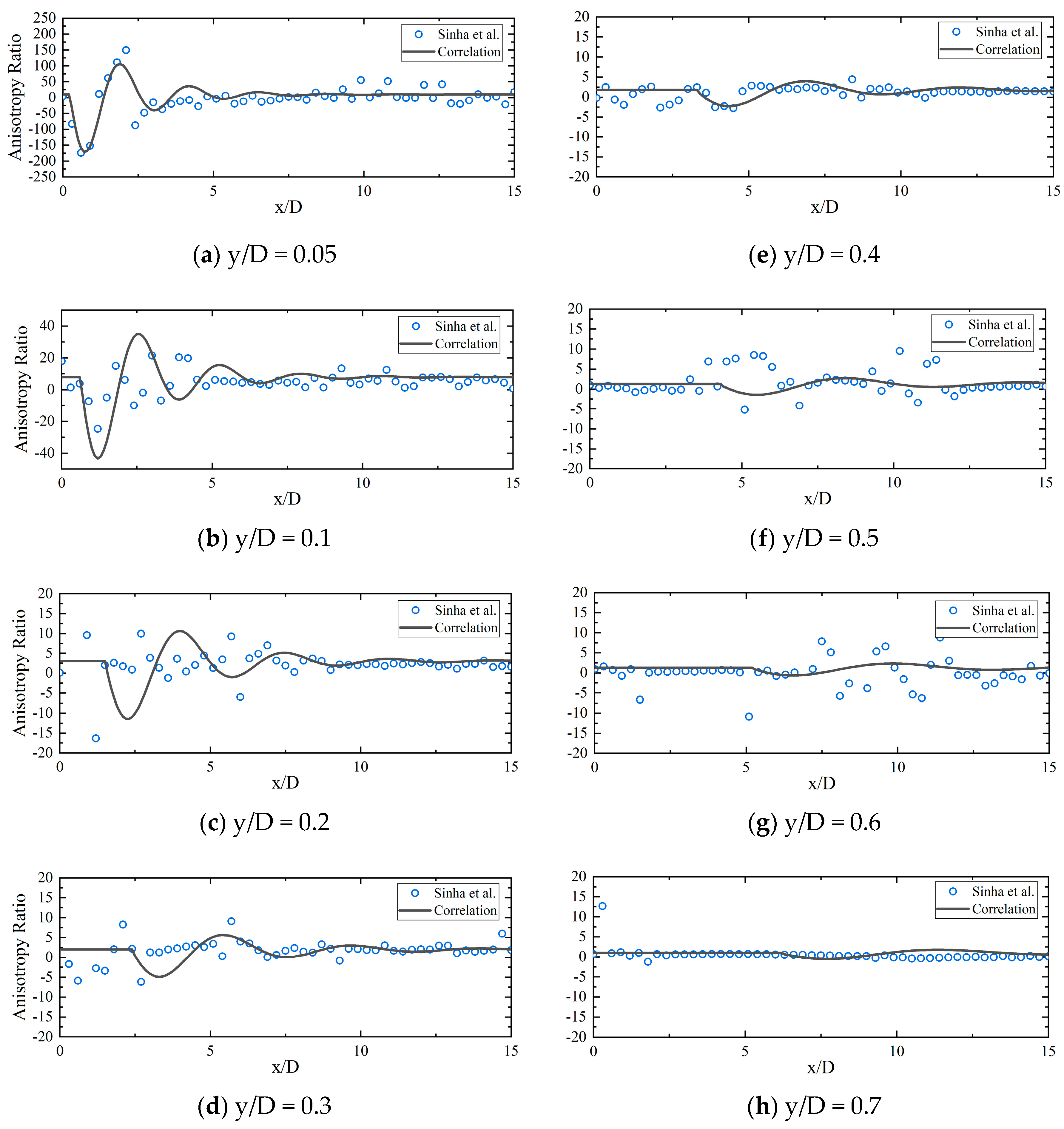
3.4. Three-Directional Anisotropy Ratio Correlation Development

To capture the strongly anisotropic eddy viscosity effect in film cooling flows, a mathematical correlation is developed to represent the anisotropy ratio f a n i s o t r o p y distributions in all three directions. As introduced above, the anisotropy ratio is large near the wall, and decreases along the wall-normal direction, as expected. As the distance to the wall decreases, u 2 decays much faster than u 3 due to the impermeable wall, which results in the eddy viscosity in the vertical direction ( ν t , y ) decreasing. Figure 13 further illustrates this point. In Figure 13, vertical lines are drawn at many different locations after the film cooling hole, and the anisotropy ratios are plotted against log y+. It is found that, before y+ of 300, the anisotropy ratio decreases with y+. After y+ of 300, the anisotropy ratio returns to a constant around 1.0, as would be expected. To follow the trend of vertical distribution of the anisotropy ratio, a correlation is proposed. The correlation assumes the log of anisotropy ratio follows a linear formula with log of y+ before y+ of 300, which can be expressed as follows:
log ν t , z ν t , y = a + b log y + ,
while the correlation returns to a constant value of 1.0 after y+ of 300. The best fitting of values a and b is obtained with all the data points, as shown in Figure 13. Thus, a correlation of f a n i s o t r o p y in the vertical direction has been obtained as follows:
f a n i s o t r o p y , y = { exp ( 3.77815 1.39985 log y + ) , y + < 300 1.0 , y + 300 .
The values given by the correlation are also plotted in Figure 13. The correlation is representative of the y-direction distribution of the anisotropy ratio.
Large oscillations of anisotropy ratio are found after y+ of 1000. The freestream turbulence intensity in the experiment is about 0.2%. Far from the wall, the Reynolds stresses become extremely small, so the anisotropy ratios are not stable in this region.
For developing the anisotropy ratio distribution in the streamwise direction, its distribution in the x direction is analyzed first. The streamwise direction distributions at various y locations are plotted in Figure 14. It can be observed in Figure 14 that the anisotropy ratio follows a damping function shape in the relatively near-field region, but approaches a small constant value of 1 far downstream. Meanwhile, at higher y locations, the damping function is initiated at a location slightly further downstream. The strong damping region seems to originate from the strong jet and crossflow interaction regions, and closely follows the trajectory of the cooling jet. The cooling jet exits the film cooling hole at y/D of 0, then the trajectory of the jet goes higher and interacts with the mainstream at higher locations as it goes farther downstream.
To capture this trend of streamwise direction distributions for anisotropy ratio, a damping dynamic system function is proposed as the fundamental formula for the correlation. A typical damping dynamic system function is defined as:
g = 1 1 β e ξ x sin ( 1 ξ 2 x + θ ) ,
where ξ is the damping ratio, and phase angle θ is defined as:
θ = tan 1 ( 1 ξ 2 ξ ) .
As seen in Figure 14, since the anisotropy ratio would first decrease then increase in the x direction, the basic formula for the damping function is modified to be:
g = g + 1 = 1 β e ξ x sin ( β x + θ ) .
For performing the function transformations to a formula that is suitable for fitting the data shown in Figure 14, four parameters, a , b , c , d are used as follows:
f a n i s o t r o p y , x = a g + b ,   x = x c d .
After the fitting of the damping ratio and the transformation parameters of a , b , c , d , a correlation of the streamwise direction distribution of the anisotropy ratio has been obtained as follows:
log ( a ) = 0.16345 1.82552 log ( y / D )
c = 0.29794 + 1.2163 ( y / D )
log ( d ) = 0.97036 + 1.07698 log ( y / D ) .
b is determined by the anisotropy ratio function in the vertical direction.
The anisotropy ratio given by the correlation has been plotted in Figure 14 as the solid line. It can be seen that, with a singular correlation, the anisotropy ratios capture well the values and trends of streamwise anisotropic eddy viscosity distributions at different y locations.
For the spanwise anisotropic eddy viscosity distributions, as shown in Figure 15, a two-peak type of distribution has been found.
To represent the two peaks’ shape anisotropic distribution in the spanwise direction, the following formula has been proposed:
f a n i s o t r o p y , z = 3 2 ( 1 2 π σ 2 e ( z / d μ ) 2 2 σ 2 + 1 2 π σ 2 e ( z / d + μ ) 2 2 σ 2 ) .
The formula is composed of two classic Gauss distributions, symmetric around the centerline of z. The averaged value of the anisotropy ratio correlation in the z direction is 1. This correlation does not change the averaged anisotropy ratio; it only changes the shape of the value. Through fitting the mean value for the distribution μ and the variance σ 2 , the spanwise direction correlation for the anisotropy ratio has been formulated as follows:
f a n i s o t r o p y , z = 3 2 ( 1 0.4 π e ( z / d 0.4 ) 2 0.4 + 1 0.4 π e ( z / d + 0.4 ) 2 0.4 ) .
Figure 15 shows the anisotropy ratio from the above correlation. It is found that the z direction correlation matches well with the trend of anisotropy ratios in different streamwise directions.
In summary, a three-directional anisotropy ratio correlation has been developed as follows:
f a n i s o t r o p y = f a n i s o t r o p y , x y f a n i s o t r o p y , z .
The anisotropy ratio correlation is then implemented into the momentum, turbulent kinetic energy, and energy equations in the URANS region of the DES model. The underprediction of eddy viscosity in the spanwise direction can be improved through the anisotropy ratio correlation. Further away from the wall, vortices are generated by the shear layer in the LES region.
For the momentum equation, eddy viscosity is multiplied by f a n i s o t r o p y in the Reynolds stress equation for the x and z directions.
u 1 u 3 ¯ = f a n i s o t r o p y ν t ( u 1 x 3 + u 3 x 1 )
In the turbulent kinetic energy equation, eddy viscosity is multiplied by f a n i s o t r o p y in the z diffusion term:
x 3 [ ( f a n i s o t r o p y ν t σ k ) k x 3 ] .
In the energy equation, eddy viscosity is multiplied by f a n i s o t r o p y in the turbulent heat flux term for the z direction:
u 3 T ¯ = f a n i s o t r o p y ν t Pr t T u 3 .

4. Modeling of the Near Field of Film Cooling with Three-Directional Eddy Viscosity Using a Modified DES Model

4.1. Computational Domain and Simulation Setup

The computational domain and test setup were based on the experimental study by Cai et al. [33]. The schematic of the experimental setup is shown in Figure 16. In Cai et al. [33]’s experiment, a test section of 40 × 40 × 200 mm was built and one row of 11 film cooling holes with a 35° inline injection angle were used. The diameter of the hole (D) is 1 mm. The distance between the neighboring hole is 3D, while the length to diameter ratio of the injection tube is around 5. The actual measurement area was a 30D long × 5D wide domain downstream, corresponding to five holes. A fast PSP technique with a frequency response of up to 6 kHz was used for the measurement. A PSP coating was deposited on the region of interest, and a high-resolution camera was used to record the luminescence intensity from the experiment. After post-processing the data with proper orthogonal decomposition (POD) analysis, instantaneous and time-averaged film cooling effectiveness fields were generated. With a constant density ratio, the film cooling effectiveness for a wide range of blowing ratios from 0.135 to 1.5 was presented and analyzed.
The computational domain was proposed accordingly. Schematics of the front and top views of the computational domain are shown in Figure 17. The computational domain for the mainstream was 36D × 20D × 3D, with a length of 6D before the hole and 30D downstream. With a mainstream velocity of 30 m/s and room-temperature conditions, three blowing ratios of 0.5, 1.0, and 1.5 under density ratio of 0.967 were simulated, corresponding to the previously introduced experiment. The freestream turbulence intensity for the cases was assumed to be 1.5%.
High-quality structured mesh, generated with ANSYS ICEM, was used in this study. As shown in Figure 18, a multiblock meshing strategy was used to comply the geometry, with “O-grid” blocking to create the mesh corresponding to the jet hole. Fine mesh is applied to the near-wall and near-field regions for capturing more turbulent structures in those regions. URANS simulation is used as a reference in a quantitative comparison of the centerline effectiveness. Mesh sensitivity testing has been performed with URANS. The simulation results yielded from 1.5 million and 2.0 million meshes showed a less than 3% difference. Thus, the 2.0 million mesh is appropriate for the URANS simulations. The DES and modified DES simulations use the same 2.0 million mesh for providing a comparison of the simulation approach. The time step is assigned to be 2.0 × 10⁻⁶ s for all the simulations. The time step meets the CFL condition to make sure that the fluid from a given mesh cell propagates only to its immediate neighbors within one time step.

4.2. Results and Discussion

Three operating conditions with a density ratio of 0.967 and blowing ratios of 0.5, 1.0, and 1.5 were studied. Simulation results were obtained with the URANS, DES, and modified DES model. The URANS results were mainly used to provide a reference for the centerline effectiveness comparison, whereas the instantaneous and time-averaged contours obtained with DES and modified DES were analyzed in detail. Figure 19 shows the side view of instantaneous dimensionless temperature contours from DES and modified DES simulations. It is seen that both the DES and modified DES models predict vortical structures, which indicates proper transformation from URANS to LES in the main flow region for the jet and mainstream interactions. As the blowing ratio increases, the momentum ratio increases, so the jet trajectory is higher. The higher trajectory enhances the mixing between the jet and mainstream. For the moderate blowing ratio of 0.5, sweeping oscillation features are seen downstream. For the higher blowing ratios of 1.0 and 1.5, the oscillations are more irregular. As the blowing ratio changes from 0.5 to 1.5, the momentum ratio increases from 0.259 to 2.327. The stronger shear between the jet and mainstream generates more eddies in high blowing ratio cases.
Figure 20 shows the front view of instantaneous dimensionless temperature contours for the three blowing ratios. The jets lift off for all three blowing ratios; the contact region between jet and blade is limited instantaneously, which means the cooling effect is not ideal near the hole. As seen in Figure 20, both models predict the asymmetric nature of the jet. The mixing between jet and mainstream is greatly enhanced for higher blowing ratios, especially for M = 1.5. This leads to insufficient cooling to the blade. The strong shear generates vortices, such that not only convection, but also advection, helps the mixing. Convection is the heat transfer due to the vortices, whereas an advection reflects the fluid transport by bulk motions, such as turbulence in the original flow and mixing between the jet and mainstream.
Figure 21 depicts the front view of time-averaged dimensionless temperature contours and velocity vectors at x/D = 5 for detailed flow structure analysis. The distance between the core of the jet and the surface increases; the averaged surface contact region decreases with increasing blowing ratio. The spanwise mixing is enhanced at higher blowing ratios. Counter-rotating vortex pairs are observed in the vector plots. The entrainment of hot gas from the mainstream to the surface is found to reduce the protective effect of the cooling jet.
Figure 22 shows the front view of time-averaged dimensionless temperature contours obtained by DES and modified DES. In Figure 22, it is seen that the spanwise mixing between the jet and mainstream is effectively enhanced by the modified DES model. The cooling jet has a higher contact area in the modified DES model, which indicates enhancement in the spanwise spreading of the CRVP. For M = 1.0 and M=1.5, the spanwise spreading of the temperature reaches the side wall at x/D = 5 and x/D = 10, which indicates that neighboring jets start to interact with each other. The modified DES model, which enhances the spanwise spreading of the CRVP and therefore the temperature diffusion, is a better approach for flat plate film cooling modeling, especially for the case of multihole film cooling modeling.
In Figure 23, the time-averaged film cooling effectiveness contours from modified DES simulations are compared with the 2D effectiveness measurements [33]. At first, similar trends could be observed in the contour for the simulation and experimental results. For M = 0.5, the modified DES results show similar film cooling effectiveness distribution before x/D = 10 compared to the measured results. After x/D = 10, the modified DES results indicated insufficient mixing of the jet and mainstream in this case. Better predictions of spanwise mixing in the downstream were observed for M = 1.0 and 1.5. For M = 1.5, the experiment shows a clear liftoff right after the hole, and the neighboring jets start to interact with each other after x/D = 10. The modified DES simulation results show similar features.
Figure 24 gives a quantitative comparison of centerline effectiveness calculated using the URANS, DES, and modified DES models with the experimental results. For M = 0.5 and M = 1.5, modified DES shows a higher centerline effectiveness compared to the DES model results, which is closer to the experimental data. The original DES model overpredicts the jets’ liftoff. The modified DES model shows better results. After x/D = 10, the modified DES model shows a lower prediction of the centerline effectiveness. As the jet reattaches to the blade surface, turbulent diffusion is more effective. URANS generally overpredicts the centerline effectiveness after the hole because it does not resolve any vortices and unsteadiness, so spanwise spreading is underestimated. A quantitative comparison of the original DES model and modified DES model has been made. Under a blowing ratio of 0.5, the DES and modified DES deviate by 62.4% and 51.5%, respectively, from the experimental data. Under a blowing ratio of 1.0, the DES and modified DES deviate by 39.8% and 26.7%, respectively, from the experimental data. Under a blowing ratio of 1.5, the DES and modified DES result in 33.5% and 28.9% deviations, respectively, from the experimental results.
Figure 25 shows the vortical structures in jet and crossflow interaction colored by dimensionless temperature from modified DES simulations. Detailed vortical structures like horseshoe, Kelvin-Helmholtz, and hairpin vortices are clearly seen in the results. It is found that the initial oscillations create the horseshoe vortices. In the near field, the rolling-up of the shear layer is predicted in the modified DES simulation, which enhances convection and advection in fluid transport. The strong shear between the jet and mainstream generates the Kelvin‒Helmholtz vortices. As the blowing ratio increases, the momentum ratio increases from 0.259 to 2.327, and more vortices are generated in higher blowing ratio cases. Another indication from Figure 25 is that more mixing is induced in the M = 1.0 and 1.5 cases, as the color is more uniform in these cases.

5. Conclusions

In this study, a three-dimensional anisotropic eddy viscosity approach is developed and used for modifying the DES model with regards to the near-field film cooling simulations. For the film cooling turbulent flow field, the jet and crossflow interactions lead to highly anisotropic and non-homogeneous eddy viscosity distribution. The spatially varied anisotropic eddy viscosity is post-processed and discussed from the point of view of the high-fidelity LES film cooling simulation results. Specifically, the Reynolds stress, eddy viscosity in different directions, and anisotropy ratio are extracted and discussed from the LES results. Then, the correlations of the anisotropy ratio in the x, y, and z directions are developed based on the anisotropy ratio distributions obtained from the LES results. The anisotropic eddy viscosity approach is proposed to be applied to the DES model for better film cooling simulations. Thus, the modified DES model is attained by implementing the three-directional anisotropic eddy viscosity correlation into the DES model. It is found that the modified DES results in better predictions in 2D and centerline effectiveness compared with the original DES model. For a quantitative comparison of the modified DES and original DES models in the centerline effectiveness prediction, the original DES yields results in 62.4%, 39.8%, and 33.5% deviations from the experimental data, respectively, while the modified DES produces 51.5%, 26.7%, and 28.9% deviations from the experimental data under blowing ratios of 0.5, 1.0, and 1.5, and a density ratio of 0.967. Better centerline effectiveness predictions of the modified DES model reflect that the modified DES enhances the spanwise spreading of the CRVP, thus improving the spanwise mixing and diffusion in film cooling simulations. Valuable predictions for the vortices’ evolution in film cooling are observed. In addition, the modified DES model matches well the 2D film cooling effectiveness experimental measurements, as well as the instantaneous and time-averaged temperature distributions.

Author Contributions

Writing–original draft, F.Y.; Writing–review & editing, S.Y. All authors have read and agreed to the published version of the manuscript.

Funding

This research received no external funding.

Conflicts of Interest

The authors declare no conflict of interest.

References

  1. Jansohn, P. Modern Gas Turbine Systems: High Efficiency, Low Emission, Fuel Flexible Power Generation; Woodhead Publishing Limited: Cambridge, UK, 2013; pp. 21–23. [Google Scholar]
  2. Hada, S.; Takata, K.; Iwasaki, Y.; Yuri, M.; Masada, J. High-efficiency gas turbine development applying 1600°C class “J” technology. Mitsubishi Heavy Ind. Tech. Rev. 2015, 52, 2–9. [Google Scholar]
  3. Ito, E.; Okada, I.; Tsukagoshi, K.; Masada, J. Development of key technologies for the next generation high temperature gas turbine. In Proceedings of the ASME Turbo Expo, Vancouver, BC, Canada, 6–10 June 2011. [Google Scholar]
  4. Han, J.C.; Ekkad, S. Recent development in turbine blade film cooling. Int. J. Rotating 2001, 7, 21–40. [Google Scholar] [CrossRef]
  5. Baldauf, S.M.; Schulz, A.; Wittig, S. High-resolution measurements of local effectiveness from discrete hole film cooling. ASME J. Turbomach 2001, 123, 758–765. [Google Scholar] [CrossRef]
  6. Han, J.C.; Dutta, S.; Ekkad, S. Gas Turbine Heat Transfer and Cooling Technology; Taylor & Francis: Boca Raton, FL, USA, 2012; pp. 225–229. [Google Scholar]
  7. Goldstein, R.J.; Jin, P.; Olson, R.L. Film cooling effectiveness and mass/heat transfer coefficient downstream of one row of discrete holes. ASME J. Turbomach. 1999, 121, 225–232. [Google Scholar] [CrossRef]
  8. Walters, D.K.; Leylek, J.H. A systematic computational methodology applied to three-dimensional film-cooling flowfield. ASME J. Turbomach. 1997, 199, 777–785. [Google Scholar] [CrossRef]
  9. Walters, D.K.; Leylek, J.H.; Buck, F.A. Film cooling on a modern HP turbine blade: Part II–compound-angle round holes. In Proceedings of the ASME Turbo Expo, Amsterdam, The Netherlands, 3–6 June 2002. [Google Scholar]
  10. Akbarzadeh, M.; Rashidi, S.; Karimi, N.; Ellahi, R. Convection of heat and thermodynamic irreversibilities in two-phase, turbulent nanofluid flows in solar heaters by corrugated absorber plates. Adv. Powder Technol. 2018, 29, 2243–2254. [Google Scholar] [CrossRef] [Green Version]
  11. Shirvan, K.M.; Ellahi, R.; Mirzakhanlari, S.; Mamourian, M. Enhancement of heat transfer and heat exchanger effectiveness in a double pipe heat exchanger filled with porous media: Numerical simulation and sensitivity analysis of turbulent fluid flow. Appl. Therm. Eng. 2016, 109, 761–774. [Google Scholar] [CrossRef]
  12. Sarafraz, M.M.; Pourmehran, O.; Yang, B.; Arjomandi, M.; Ellahi, R. Pool boiling heat transfer characteristics of iron oxide nano-suspension under constant magnetic field. Int. J. Therm. Sci. 2020, 147, 106131. [Google Scholar] [CrossRef]
  13. Ray, A.K.; Vasu, B.; Bég, O.A.; Gorla, R.S.; Murthy, P.V.S.N. Homotopy semi-numerical modeling of non-Newtonian nanofluid transport external to multiple geometries using a revised Buongiorno Model. Inventions 2019, 4, 54. [Google Scholar] [CrossRef] [Green Version]
  14. Compton, D.A.; Eaton, J.K. Near-wall measurements in a three-dimensional turbulent boundary layer. ASME J. Fluid Mech. 1997, 350, 189–208. [Google Scholar] [CrossRef]
  15. Kaszeta, R.W.; Simon, T.W. Measurement of eddy diffusivity of momentum in film cooling flows with streamwise injection. ASME J. Turbomach. 1999, 122, 178–183. [Google Scholar] [CrossRef]
  16. Coletti, F.; Benson, M.J.; Ling, J.; Elkins, C.J.; Eaton, J.K. Turbulent transport in an inclined jet in crossflow. Int. J. Heat Fluid Flow 2013, 43, 149–160. [Google Scholar] [CrossRef]
  17. Ling, J.; Templeton, J. Evaluation of machine learning algorithms for prediction of regions of high Reynolds averaged Navier Stokes uncertainty. Phys. Fluids 2015, 27, 085103. [Google Scholar] [CrossRef]
  18. Dow, E.; Wang, Q. Uncertainty quantification of structural uncertainties in RANS simulations of complex flows. In Proceedings of the AIAA Computational Fluid Dynamics Conference, Honolulu, HI, USA, 27–30 June 2011. [Google Scholar]
  19. Acharya, S.; Tyagi, M.; Hoda, A. Flow and heat transfer predictions for film cooling. Ann. N. Y. Acad. Sci. 2001, 934, 110–125. [Google Scholar] [CrossRef] [PubMed]
  20. Kapadia, S.; Roy, S.; Heidmann, J. Detached eddy simulation of turbine blade cooling. In Proceedings of the 36th AIAA Thermophysics Conference, Orlando, FL, USA, 23–26 June 2003. [Google Scholar]
  21. Spalart, P.R.; Streett, C. Young-person’s guide to detached-eddy simulation grids. NASA CR-2001-211032.
  22. Squires, K.D.; Forsythe, J.R.; Morton, S.A.; Strang, W.Z.; Wurtzler, K.E.; Tomaro, R.F.; Grismer, M.J.; Spalart, P.R. Progress on detached-eddy simulation of massively separated flows. In Proceedings of the 40th AIAA Aerospace Sciences Meeting & Exhibit, Reno, NV, USA, 14–17 January 2002. [Google Scholar]
  23. Fröhlich, J.; Terzi, D.V. Hybrid LES/RANS methods for the simulation of turbulent flows. Prog. Aerosp. Sci. 2008, 44, 349–377. [Google Scholar] [CrossRef]
  24. Spalart, P.R. Detached-eddy simulation. Annu. Rev. Fluid Mech. 2009, 41, 181–202. [Google Scholar] [CrossRef]
  25. Yu, F.; Yavuzkurt, S. Simulation of film cooling flow structure and heat transfer in the near field of cooling jets with a modified DES model. In Proceedings of the ASME SHTC, Bellevue, WA, USA, 12–15 July 2019. [Google Scholar]
  26. Roy, S.; Kapadia, S.; Heidmann, J.D. Film cooling analysis using des turbulence model. In Proceedings of the ASME Turbo Expo, Atlanta, GA, USA, 16–19 June 2003. [Google Scholar]
  27. Sakai, E.; Takahashi, T.; Funazaki, K.I.; Salleh, H.B.; Watanabe, K. Numerical study on flat plate and leading edge film cooling. In Proceedings of the ASME Turbo Expo, Orlando, FL, USA, 8–12 June 2009. [Google Scholar]
  28. Ling, J.; Ryan, K.J.; Bodart, J.; Eaton, J.K. Analysis of turbulent scalar flux models for a discrete hole film cooling flow. J. Turbomach. 2016, 138, 011006. [Google Scholar] [CrossRef]
  29. Milani, P.M.; Ling, J.; Saez-Mischlich, G.; Bodart, J.; Eaton, J.K. A machine learning approach for determining the turbulent diffusivity in film cooling flows. J. Turbomach. 2018, 140, 021006. [Google Scholar] [CrossRef] [Green Version]
  30. Gritsch, M.; Colban, W.; Schär, H.; Döbbeling, K. Effect of hole geometry on the thermal performance of fan-shaped film cooling holes. J. Turbomach. 2005, 127, 718–725. [Google Scholar] [CrossRef]
  31. Schroeder, R.P.; Thole, K.A. Adiabatic effectiveness measurements for a baseline shaped film cooling hole. In Proceedings of the ASME Turbo Expo, Düsseldorf, Germany, 16–20 June 2014. [Google Scholar]
  32. Zuniga, H.A.; Kapat, J.S. Effect of increasing pitch-to-diameter ratio on the film cooling effectiveness of shaped and cylindrical holes embedded in trenches. In Proceedings of the ASME Turbo Expo, Orlando, FL, USA, 8–12 June 2009. [Google Scholar]
  33. Cai, T.; Peng, D.; Yavuzkurt, S.; Liu, Y.Z. Unsteady 2-D film-cooling effectiveness behind a single row of holes at different blowing ratios: Measurements using fast-response pressure-sensitive paint. Int. J. Heat Mass Transfer 2018, 120, 1325–1340. [Google Scholar] [CrossRef]
  34. Shih, T.; Liou, W.; Shabbir, A.; Yang, Z.; Zhu, J. A New k-epsilon Eddy-Viscosity Model for High Reynolds Number Turbulent Flows—Model Development and Validation. Comput. Fluids 1995, 24, 227–238. [Google Scholar] [CrossRef]
  35. Fluent, ANSYS. 12.0 Theory Guide; Ansys Inc: Canonsburg, PA, USA, 2009.
  36. Han, J.C.; Rallabandi, A. Turbine blade film cooling using PSP technique. FHMT 2010, 1, 013001. [Google Scholar] [CrossRef]
  37. Wright, L.M.; Gao, Z.; Varvel, T.A.; Han, J.C. Assessment of steady state PSP, TSP, and IR measurement techniques for flat plate film cooling. In Proceedings of the ASME Summer Heat Transfer Conference collocated with the ASME Pacific Rim Technical Conference and Exhibition on Integration and Packaging of MEMS, NEMS, and Electronic Systems, San Francisco, CA, USA, 17–22 July 2005. [Google Scholar]
  38. Rallabandi, A.P.; Li, S.J.; Han, J.C. Unsteady Wake and Coolant Density Effects on Turbine Blade Film Cooling Using Pressure Sensitive Paint Technique. J. Heat Transf. 2012, 134, 081701. [Google Scholar] [CrossRef]
  39. Moin, P.; Mahesh, K. Direct numerical simulation: A tool in turbulence research. Annu Rev. Fluid Mech. 1998, 30, 539–578. [Google Scholar] [CrossRef] [Green Version]
  40. Sinha, A.K.; Bogard, D.G.; Crawford, M.E. Film-cooling effectiveness downstream of a single row of holes with variable density ratio. ASME J. Turbomach. 1991, 113, 442–449. [Google Scholar] [CrossRef]
Figure 1. Test section used in the experiment. Modified from Compton and Eaton [14] (dimensions in inches).
Inventions 05 00013 g001
Figure 2. Mesh for the whole test section.
Inventions 05 00013 g002
Figure 3. Mesh for the rear part of the test section.
Inventions 05 00013 g003
Figure 4. Comparison of angles of stress and strain at x = 0.4445 m, z = 0.0 obtained from LES model results and experimental data [14].
Inventions 05 00013 g004
Figure 5. Top view of time-averaged strain rates, u 1 u 2 ¯ , u 1 u 3 ¯ Reynolds stresses, eddy viscosity in y, z direction, anisotropy ratio, and film cooling effectiveness at y/D = 0.1 plane obtained using LES.
Inventions 05 00013 g005
Figure 6. Top view of time-averaged strain rate, u 1 u 2 ¯ , u 1 u 3 ¯ Reynolds stresses, eddy viscosity, and film cooling effectiveness at y/D = 0.1 plane obtained using URANS.
Inventions 05 00013 g006
Figure 7. Spanwise distribution of film cooling effectiveness obtained from URANS and LES models at x/D = 15 for DR = 2, M = 1.
Inventions 05 00013 g007
Figure 8. Front view of time-averaged strain rate, u 1 u 2 ¯ , u 1 u 3 ¯ Reynolds stress, eddy viscosity, and film cooling effectiveness obtained using LES for x/D = 5 plane.
Inventions 05 00013 g008
Figure 9. Front view of time-averaged strain rate, u 1 u 2 ¯ , u 1 u 3 ¯ Reynolds stress, eddy viscosity, and film cooling effectiveness obtained using URANS for x/D = 5 plane.
Inventions 05 00013 g009
Figure 10. Top view of time-averaged strain rate, u 1 u 2 ¯ , u 1 u 3 ¯ Reynolds stresses, eddy viscosity in y, z direction, anisotropy ratio, and film cooling effectiveness obtained using LES for y/D = 0.05 plane.
Inventions 05 00013 g010
Figure 11. Top view of time-averaged strain rate, u 1 u 2 ¯ , u 1 u 3 ¯ Reynolds stresses, eddy viscosity in y, z direction, anisotropy ratio, and film cooling effectiveness obtained using LES for y/D = 0.5 plane.
Inventions 05 00013 g011
Figure 12. Top view of time-averaged strain rate, u 1 u 2 ¯ , u 1 u 3 ¯ Reynolds stresses, eddy viscosity in y, z direction, anisotropy ratio, and film cooling effectiveness obtained using LES for y/D = 1.0 plane.
Inventions 05 00013 g012
Figure 13. Anisotropy ratio correlation in the vertical direction.
Inventions 05 00013 g013
Figure 14. Anisotropy ratio correlation in streamwise direction.
Inventions 05 00013 g014
Figure 15. Anisotropy ratio correlation in spanwise direction.
Inventions 05 00013 g015
Figure 16. Schematic of the experimental setup from Cai et al. [33] and the computational domain used in this study.
Inventions 05 00013 g016
Figure 17. Schematic of the front and top view of the computational domain.
Inventions 05 00013 g017
Figure 18. Mesh for plenum, film cooling tubes, and mainstream.
Inventions 05 00013 g018
Figure 19. Side view of instantaneous dimensionless temperature contours for M = 0.5, 1.0, and 1.5 in the center plane obtained using DES and modified DES models.
Inventions 05 00013 g019
Figure 20. Front view of instantaneous dimensionless temperature contours at (a) x/D = 5, (b) x/D = 10, (c) x/D = 15 obtained by the DES and modified DES models.
Inventions 05 00013 g020
Figure 21. Front view of time-averaged dimensionless temperature contours overlaid with time-averaged velocity vectors at x/D = 5 obtained using modified DES.
Inventions 05 00013 g021
Figure 22. Front view of time-averaged dimensionless temperature contours at (a) x/D = 5, (b) x/D = 10, (c) x/D = 15 obtained using the DES and modified DES models.
Inventions 05 00013 g022aInventions 05 00013 g022b
Figure 23. Top view of time-averaged film cooling effectiveness contours for (a) M = 0.5, (b) M = 1.0, (c) M = 1.5 obtained using the modified DES model and Cai et al. [33].
Inventions 05 00013 g023aInventions 05 00013 g023b
Figure 24. Comparison of centerline effectiveness from the URANS, DES, and modified DES models with the experimental results [33] for (a) M = 0.5, (b) M = 1.0, and (c) M = 1.5.
Inventions 05 00013 g024aInventions 05 00013 g024b
Figure 25. Vortices generated during jet and crossflow interaction, colored by dimensionless temperature, obtained using the modified DES model.
Inventions 05 00013 g025

