Temperature Distribution through a Nanofilm by Means of a Ballistic-Diffusive Approach

Abstract

As microelectronic devices are important in many applications, their heat management needs to be improved, in order to prolong their lifetime, and to reduce the risk of damage. In nanomaterials, heat transport shows different behaviors than what can be observed at macroscopic sizes. Studying heat transport through nanofilms is a necessary tool for nanodevice thermal management. This work proposes a thermodynamic model incorporating both ballistic, introduced by non-local effects, and diffusive phonon transport. Extended thermodynamics principles are used in order to develop a constitutive equation for the ballistic behavior of heat conduction at small-length scales. Being an irreversible process, the present two-temperature model contains a one-way transition of ballistic to diffusive phonons as time proceeds. The model is compared to the classical Fourier and Cattaneo laws. These laws were not able to present the non-locality that our model shows, which is present in cases when the length scale of the material is of the same order of magnitude or smaller than the phonon mean free path, i.e., when the Knudsen number $Kn\le O\left(1\right)$. Moreover, for small $Kn$ numbers, our model predicted behaviors close to that of the classical laws, with a weak temperature jump at both sides of the nanofilm. However, as $Kn$ increases, the behavior changes completely, the ballistic component becomes more important, and the temperature jump at both sides of the nanofilms becomes more pronounced. For comparison, a model using Fourier’s and Cattaneo’s laws with an effective thermal conductivity has shown, with reasonable qualitative comparison for small Knudsen numbers and large times.

1. Introduction

An increasing attention towards nanotechnology has yielded new developments concerning transport phenomena in nanomaterials. It is well known that heat transfer at micro- and nanoscales shows different behaviors from that at macroscales [1,2]. Thermal management is important, due to the miniaturization of electronic devices, which necessitates more attention, to prevent overheating [3]. Local hotspots can reduce remarkably the lifetimes of such electronic devices, and even cause damage to those devices [4,5]. Other studies that investigate thermal management of devices at the nanoscale include the cooling of microfluidic electronic systems [6], enhancing the thermal conductance of 2D materials [7], and improving the efficiency of thermoelectric devices [8], to mention a few. Modelling can provide useful information [9], in order to attain the aforementioned objectives, whether they be sought after or refrained from. Quite some modelling work has been performed in analyzing thermal management in nanofilms or devices at the nanoscale. Works on phonon transport in silicon nanofilms [10,11] make use of numerical methods for predicting thermal conductance. More specific numerical methods are also employed, such as non-equilibrium molecular dynamics [12], the often-used phonon Boltzmann equation [13], and also phonon hydrodynamics [14]. These studies do not make the distinction between the different types of phonon carriers. Indeed, as the characteristic size of the system becomes of the order of magnitude of the phonon mean free path, ballistic features begin to play a role. To account for the ballistic effects, some studies proposed ballistic-diffusive phonon transport via Monte Carlo simulations [15,16]. Other works regarded the ballistic-type of phonon transport as an introduction of a non-local effect, obtaining via the phonon Boltzmann equation the Guyer–Krumhansl equation [17,18,19]. Whilst these works appeared to provide quite correct predictions (and as will be mentioned later, our model will give comparable results), these works either demand a high computing cost [15,16], or they lack the distinction between the diffusive and ballistic components [17,18,19]. Although they do not make an explicit distinction between the ballistic and diffusive components, this does not necessarily mean that the model is incorrect (it can indeed predict correctly); such a distinction can provide more information on the behavior of the phonons. The model that we propose in this work contains both non-local effects, and makes distinctions between the diffusive and ballistic components. Furthermore, it will be developed from thermodynamic principles (and not from numerical nor kinetic bases), which makes it easily connectable to other physical phenomena, such as mass transport, electric current, and so on [1]. In a greater framework, this work would fit easily without great adaptations nor high computing efforts.

Whether heat transport is of diffusive of a ballistic nature depends mainly on the size of the system. A typical way to make a rough quantitative distinction between these two heat transport mechanisms is the so-called Knudsen number $Kn\equiv \mathcal{l}/L$, where $\mathcal{l}$ denotes the mean free path of the carriers in question (phonons in case of heat transfer) and $L$ a characteristic dimension of the system under study. For large Knudsen numbers (typically larger than one), the heat transport is referred to as ballistic, i.e., dominated by phonon collisions with the walls. If the Knudsen number is much smaller than one, heat transport is simply diffusive, i.e., dominated by phonon–phonon collisions inside the system, and described by Fourier’s law. For small-length systems (of the order of magnitude of the mean free path of the carrier or smaller), as well as for high-frequency processes (of which the inverse is of the order of magnitude of the relaxation time of the carrier or smaller), Fourier’s law is no longer valid. These observations justify the need to propose a constitutive law that generalizes Fourier’s law, emanating from extended well-known established thermodynamic laws. Although there are various ways by which this can be achieved [20,21,22], we prefer to present a solution that is easily connectable with existing balance equations, and recognizable with more simplified constitutive equations. The classical Fourier law:

$$\mathit{q}=-\lambda \nabla T,$$

(1)

relating the heat flux vector $\mathit{q}$ to the temperature gradient $\nabla T$, with $\lambda$ denoting the thermal conductivity, is not applicable at short time periods and small spatial scales. In order to account for high frequencies, Fourier’s law has been generalized by Cattaneo [23] under the form:

$$\tau {\partial }_t\mathit{q}+\mathit{q}=-\lambda \nabla T,$$

(2)

with $\tau$ designating the relaxation time of the heat flux and ${\partial }_t$ the partial time derivative. Nonetheless, Cattaneo’s relation cannot be used for nanosystems. For this, we propose an extended, generalized constitutional equation for heat conduction, which is valid for nanosystems, systems with high frequencies, and systems with large relaxation times. For this, we use Extended Non-Equilibrium Thermodynamics [1,24], proposing a procedure that can be easily generalized to other transport phenomena, such as electrical conduction and matter diffusion, but we limit ourselves here to heat transport. Applied to heat transport, the theory has as main characteristic to upgrade the heat flux, and higher-order heat fluxes to the rank of independent variables as the internal energy (temperature). The obtained result will then be of use for describing ballistic heat transport, when we propose a two-temperature model, in order to describe heat transport through a thin slab. At the end, a comparison is made with Fourier’s and Cattaneo’s laws, adapted with a developed effective thermal conductivity.

2. Methods: Constitutional Equation for Ballistic Heat Transport

For rigid material, we can define an entropy function $𝓈$. Let us assume that this entropy $𝓈\left(u,\mathit{q}\right)$ is depending on both the internal energy $u$ and the heat flux vector $\mathit{q}$. The corresponding Gibbs equation in a rigid conductor (i.e., $d_t\equiv {\partial }_t$) at rest writes as:

$${\partial }_t𝓈\left(u,\mathit{q}\right)=T^{-1}{\partial }_{t}u-{\gamma }_1\mathit{q}.{\partial }_t\mathit{q},$$

(3)

wherein $𝓈$ and $u$ are measured per unit volume, ${\gamma }_1$ is a phenomenological coefficient assumed to be independent of $\mathit{q}$, and a dot stands for the scalar product. The coefficient ${\gamma }_1$ will be identified later on, where it will be shown to be related to the relaxation time $\tau$ and the thermal conductivity $\lambda$. It should be noted that (3) does not take into account any terms that allow for coping with non-local effects, which are dominant at small length scales. To take them into account, it is suggested to introduce a hierarchy of fluxes ${\mathit{Q}}^{\left(1\right)}$, ${\mathit{Q}}^{\left(2\right)}$,..., ${\mathit{Q}}^{\left(n\right)}$ with ${\mathit{Q}}^{\left(1\right)}$ being identical to the heat flux vector $\mathit{q}$, where ${\mathit{Q}}^{\left(2\right)}$ (a tensor of rank two) is the flux of $\mathit{q}$, ${\mathit{Q}}^{\left(3\right)}$ the flux of ${\mathit{Q}}^{\left(2\right)}$, and so on. Up to the $N^{th}$-order flux, the generalized Gibbs equation can then be written as:

$${\partial }_t𝓈\left(u,\mathit{q},{\mathit{Q}}^{\left(1\right)},\dots ,{\mathit{Q}}^{\left(n\right)}\right)=T^{-1}{\partial }_{t}u-{\gamma }_1\mathit{q}·{\partial }_t\mathit{q}-{\gamma }_2{\mathit{Q}}^{\left(2\right)}⨂{\partial }_t{\mathit{Q}}^{\left(2\right)}-\dots -{\gamma }_n{\mathit{Q}}^{\left(n\right)}⨂{\partial }_t{\mathit{Q}}^{\left(n\right)},$$

(4)

wherein the symbol $⨂$ denotes the inner product of the corresponding tensors, and $n=2,3,\dots N$. Moreover, the time evolution of the entropy is governed by a general balance equation, which can be written as:

$${\eta }^s={\partial }_t𝓈+\nabla ·{\mathit{J}}^s\ge 0,$$

(5)

wherein ${\mathit{J}}^s$ stands for the entropy flux and ${\eta }^s$ for the rate of entropy production per unit volume, which is positive definite to fulfil the second law of thermodynamics. In order to deduce an expression for ${\eta }^s$, we use (4) for ${\partial }_t𝓈$, and we need a constitutive relation for ${\mathit{J}}^s$ in terms of the set of variables established earlier. It is natural to expect that ${\mathit{J}}^s$ is not simply given by the classical expression $T^{-1}\mathit{q}$ [25], but that it will depend on all the higher order fluxes up to order $n$, namely:

$${\mathit{J}}^s=T^{-1}\mathit{q}+{\beta }_1{\mathit{Q}}^{\left(2\right)}·\mathit{q}+\dots +{\beta }_{n-1}{\mathit{Q}}^{\left(n\right)}⨂{\mathit{Q}}^{\left(n-1\right)},$$

(6)

with ${\beta }_n$ designating the phenomenological coefficients. We substitute in (5) the expressions of ${\partial }_t𝓈$ and ${\mathit{J}}^s$ by (4) and (6), respectively. We then replace derivative ${\partial }_{\mathrm{t}}\mathrm{u}$ by the energy conservation law, ${\partial }_{t}u=-\nabla ·\mathit{q}$, which leads to the expression for the entropy production:

$${\eta }^s=-\left(-\nabla T^{-1}+{\gamma }_1{\partial }_t\mathit{q}-{\beta }_1\nabla ·{\mathit{Q}}^{\left(2\right)}\right)·\mathit{q}\dots -{\displaystyle \sum }_{n=2}^N{\mathit{Q}}^{\left(n\right)}⨂\left({\gamma }_n{\partial }_t{\mathit{Q}}^{\left(n\right)}-{\beta }_n\nabla ·{\mathit{Q}}^{\left(n+1\right)}-{\beta }_{n-1}\nabla {\mathit{Q}}^{\left(n-1\right)}\right)\ge 0$$

(7)

The above is a bilinear expression in fluxes and forces (the quantities between parentheses), which suggests the following hierarchy of linear flux–force relations:

$$\nabla T^{-1}-{\gamma }_1{\partial }_t\mathit{q}+{\beta }_1\nabla ·{\mathit{Q}}^{\left(2\right)}={\nu }_1\mathit{q}$$

(8)

$${\beta }_{n-1}\nabla {\mathit{Q}}^{\left(n-1\right)}-{\gamma }_n{\partial }_t{\mathit{Q}}^{\left(n\right)}+{\beta }_n\nabla ·{\mathit{Q}}^{\left(n+1\right)}={\nu }_n{\mathit{Q}}^{\left(n\right)}(n=2,3,\dots N)$$

(9)

It is the purpose to replace the set of relations (8)–(9) by one single constitutive equation that takes into account all the $N^{th}$ order fluxes. For the sake of clarity, we will make the development up to the fourth order, and generalize afterwards. The fourth order flux equation ($n=4$ in Equation (9)) is given by:

$${\beta }_3\nabla {\mathit{Q}}^{\left(3\right)}-{\gamma }_4{\partial }_t{\mathit{Q}}^{\left(4\right)}+{\beta }_4\nabla ·{\mathit{Q}}^{\left(5\right)}={\nu }_4{\mathit{Q}}^{\left(4\right)}$$

(10)

Let us now take the divergence ($\nabla$) of (10), substituting it subsequently in (9), with $n=3$, and omitting any flux, $n>4$. This gives:

$${\beta }_2\nabla {\mathit{Q}}^{\left(2\right)}-{\gamma }_3{\partial }_t{\mathit{Q}}^{\left(3\right)}+\frac{{\beta }_3}{{\nu }_4}\left({\beta }_3\nabla ·\nabla {\mathit{Q}}^{\left(3\right)}-{\gamma }_4\nabla ·{\partial }_t{\mathit{Q}}^{\left(4\right)}\right)={\nu }_3{\mathit{Q}}^{\left(3\right)}$$

(11)

Applying again operator divergence on (11), substituting it on its turn in (9) but with $n=2$ and repeating the same operation until arriving at Equation (9) with $n=1$ (the latter of which is equivalent to Equation (8)), the final result is:

$$\begin{gathered} \nabla T^{-1}-{\gamma }_1{\partial }_t\mathit{q}+\frac{{\beta }_1}{{\nu }_2}\left({\beta }_1\nabla ·\nabla \mathit{q}-{\gamma }_2\nabla ·{\partial }_t{\mathit{Q}}^{\left(2\right)}+\frac{{\beta }_2}{{\nu }_3}\left({\beta }_2\nabla ·\nabla ·\nabla {\mathit{Q}}^{\left(2\right)}-{\gamma }_3\nabla ·\nabla ·{\partial }_t{\mathit{Q}}^{\left(3\right)} \\ +\frac{{\beta }_3}{{\nu }_4}\left({\beta }_3\nabla ·\nabla ·\nabla ·\nabla {\mathit{Q}}^{\left(3\right)}-{\gamma }_4\nabla ·\nabla ·\nabla ·{\partial }_t{\mathit{Q}}^{\left(4\right)}\right)\right)\right)={\nu }_1\mathit{q} \end{gathered}$$

(12)

This relation may be viewed as a generalization of Fourier’s and/or Cattaneo’s relation, up to the fourth-order flux ${\mathit{Q}}^{\left(4\right)}$. However, the use of higher order fluxes is not very convenient from a practical point of view, since their physical meaning, being not directly measurable, is not clear. This calls for proposing a more suitable representation, wherein all the high-order fluxes have been expressed solely in the heat flux.

Therefore, the purpose is to express Equation (12) exclusively in terms of the more physical quantities, the temperature $T$ and the classical heat flux $\mathit{q}$. The higher-order fluxes ${\mathit{Q}}^{\left(n\right)}$ are eliminated by making use of the very definition of the high-order flux, namely:

$${\partial }_t{\mathit{Q}}^{\left(n\right)}=-\nabla ·{\mathit{Q}}^{\left(n+1\right)}(n=1,2,3,\dots N)$$

(13)

In virtue of (13) and after some rearrangements, Equation (12) can be rewritten as:

$$\begin{array}{ll}\frac{{\gamma }_1}{{\nu }_1}{\partial }_t\mathit{q}+\mathit{q}=& -\frac{1}{{\nu }_1{T}^2}\nabla T+\frac{1}{{\nu }_1}\frac{{\beta }_1}{{\nu }_2}{\beta }_1{\nabla }^2\mathit{q}+\frac{1}{{\nu }_1}\frac{{\beta }_1}{{\nu }_2}{\gamma }_2{\partial }_t{\partial }_t\mathit{q}-\frac{1}{{\nu }_1}\frac{{\beta }_1}{{\nu }_2}\frac{{\beta }_2}{{\nu }_3}{\beta }_2{\partial }_t{\nabla }^2\mathit{q}\\ & -\frac{1}{{\nu }_1}\frac{{\beta }_1}{{\nu }_2}\frac{{\beta }_2}{{\nu }_3}{\gamma }_3{\partial }_t{\partial }_t{\partial }_t\mathit{q}+\frac{1}{{\nu }_1}\frac{{\beta }_1}{{\nu }_2}\frac{{\beta }_2}{{\nu }_3}\frac{{\beta }_3}{{\nu }_4}{\beta }_3{\partial }_t{\partial }_t{\nabla }^2\mathit{q}\\ & +\frac{1}{{\nu }_1}\frac{{\beta }_1}{{\nu }_2}\frac{{\beta }_2}{{\nu }_3}\frac{{\beta }_3}{{\nu }_4}{\gamma }_4{\partial }_t{\partial }_t{\partial }_t{\partial }_t\mathit{q}\end{array}$$

(14)

By extending the exercise to higher-order fluxes with $n=N$ (where theoretically, $N\to \infty$, but practically often not necessary), we obtain the following general equation governing heat conduction in rigid bodies:

$$\begin{gathered} \frac{{\gamma }_1}{{\nu }_1}{\partial }_t\mathit{q}+\mathit{q}=-\frac{1}{{\nu }_1{T}^2}\nabla T+\frac{1}{{\nu }_1}{{\displaystyle \sum }}_{n=1}^N\left(\left({{\displaystyle \prod }}_{i=1}^n\frac{{\beta }_i}{{\nu }_{i+1}}\right){\left(-1\right)}^{n+1}{\beta }_n\frac{{\partial }^{n-1}}{\partial t^{n-1}}{\nabla }^2\mathit{q}+ \\ \left({{\displaystyle \prod }}_{i=1}^n\frac{{\beta }_i}{{\nu }_{i+1}}\right){\left(-1\right)}^{n+1}{\gamma }_{n+1}\frac{{\partial }^{n+1}}{\partial t^{n+1}}\mathit{q}\right) \left(n=1,2,3,\dots ,N\right), \mathrm{with}N\in {\mathbb{N}}^{+} \end{gathered}$$

(15)

Setting ${\gamma }_1={\beta }_1=0$, Equation (8) reduces to Fourier’s law, from which it follows that ${\nu }_1=\frac{1}{\lambda T^2}$. Comparing the unities in (8) indicates that the dimension of the ratio ${\gamma }_1/{\nu }_1$ is that of time ($t$), so that $\left[{\gamma }_1\right]=\left[t\right]\left[{\nu }_1\right]$. Defining the time unit as the heat flux ($\mathit{q}$) and relaxation time ${\tau }_1$, one has ${\gamma }_1={\tau }_1{\nu }_1=\frac{{\tau }_1}{\lambda T^2}$. As the heat flux $\mathit{q}$ is expressed in W/m², the unity of ${\mathit{Q}}^{\left(2\right)}$ is W/(m·s), according to (13): $\left[{\mathit{Q}}^{\left(n+1\right)}\right]=\frac{\left[L\right]}{\left[t\right]}\left[{\mathit{Q}}^{\left(n\right)}\right]$, where [$L$] is a unity in length. As a direct consequence of the property that ${\mathit{Q}}^{\left(2\right)}$ is the flux of $\mathit{q}$, one has in (8) that $\frac{{\beta }_1}{{\gamma }_1}=-1$ or ${\beta }_1=-{\gamma }_1=-{\tau }_1{\nu }_1$. For further application, we neglect higher orders of the relaxation times, i.e., ${\tau }_2={\tau }_3=\dots ={\tau }_n=0$, which means that the phenomenological coefficients ${\beta }_n$ and ${\gamma }_n$, with $n\ge 2$, and ${\nu }_n$, and $n\ge 3$ (note that although ${\beta }_2$ and ${\gamma }_2$ are related to ${\tau }_2$, ${\nu }_2$ is rather related to ${\tau }_1$), can be omitted. Equation (15) becomes:

$$\tau {\partial }_t\mathit{q}+\mathit{q}=-\lambda \nabla T+{\mathcal{l}}^2{\nabla }^2\mathit{q}$$

(16)

We can see clearly differences between (16) and the conventional constitutional laws for heat transport (1) and (2), but also some similarities. For systems where its characteristic size is much larger than the mean free path $\mathcal{l}$, Equation (16) reduces to Cattaneo’s equation. This corresponds also to neglecting any higher order of heat fluxes (reducing the whole deduction in this section to only Equations (3) and (5), with ${\mathit{J}}^s=T^{-1}\mathit{q}$). If, furthermore, the changes in the heat flux occur in a time span that is much larger than the relaxation time, we obtain Fourier’s law. Other well-known methods that are used, as those mentioned in the Introduction, comprise the phonon–Boltzmann equation, the Monte Carlo simulations, and Molecular Dynamics. The Monte Carlo simulations and Molecular Dynamics methods do not require higher-order variables, but they demand high computing times, and are not flexible for modelling various scales at a time, although efforts have been performed in performing multi-scale molecular dynamics [26]. Solving the phonon–Boltzmann equation also asks for a high computational time. These are issues that are not a problem for the model presented in this work. However, the definition of the ballistic and diffusive temperatures is not well-defined, which limits direct interpretation. This can be circumvented by noticing that the ballistic and diffusive temperatures are actually defined through their respective internal energies. Assuming that the total internal energy is a measure for the real temperature, the evaluation of the total temperature becomes, therefore, correct. Assuming also that the ballistic and diffusive internal energies sum up linearly to obtain the total internal energy, allows for an interpretation of the contribution of the ballistic and diffusive phonon regimes via the internal energies. The present development could, of course be extended by introducing non-linear heat fluxes. However, such an extension, albeit theoretically not an issue, would be numerically cumbersome to perform, also inducing also boundary conditions that may not be well defined. Non-linear contributions of the heat flux (at first and higher orders) could be important when the length scale becomes much smaller than the mean free path of the phonons. Nevertheless, for most materials, a linear heat flux consideration still gives satisfactory results [1,27], making it very reasonable and consistent to use linear heat fluxes for predicting material properties in several applications.

3. Temperature Distribution in Nanoscaled Materials

We have discussed that, depending on the size, the type of heat transfer can be either ballistic or diffusive. In order to appreciate the contribution of both the ballistic and diffusive parts of the heat flux, we propose a two-temperature model.

3.1. Two-Temperature Model

In order to find the temperature distribution, we need to assume the coexistence of two kinds of heat carriers: diffusive phonons which undergo multiple collisions within the core of the system, and ballistic phonons originating at the boundaries and experiencing collisions with the walls. This representation is called the ballistic-diffusion model. As such, the internal energy and the heat flux are decomposed into a ballistic and a diffusive component, which gives $u =u_b+u_d$ and $\mathit{q} ={\mathit{q}}_b+{\mathit{q}}_d$, where the indexes $b$ and $d$ refer to ballistic and diffusive contributions, respectively. The space of state variables is constituted by the quantities $u_d$, $u_b$,${\mathit{q}}_d$ and ${\mathit{q}}_b$. Let us introduce the diffusive and ballistic temperatures $T_d$ and $T_b$, defined respectively by $T_d=u_d/c_d$ and $T_b=u_b/c_b$, where $c_d$ and $c_b$ stand for the heat capacity per unit volume, and are positive quantities to guarantee the stability of the equilibrium state. Stating that $c_d=c_b=c$, leading to the total temperature being defined by $T= u/c$, or equivalently, $T= T_d+T_b$. Although the quantities $T_d$ and $T_b$ bear some analogy with the classical definition of the temperature, it should however, be realized that, strictly speaking, these quantities do not represent temperatures in the usual sense, but must be considered as a measure of the internal energies.

After having defined the state variables, we specify their behavior in the course of time and space. The evolutions of the internal energies $u_d$ and $u_b$, are governed by the classical energy balance laws:

$$\frac{\partial u_d}{\partial t}=-\nabla ·{\mathit{q}}_d+r_d$$

(17)

$$\frac{\partial u_b}{\partial t}=-\nabla ·{\mathit{q}}_b+r_b$$

(18)

while the total internal energy $u= u_d+u_b$ satisfies the first law of thermodynamics:

$$\frac{\partial u}{\partial t}=-\nabla ·\mathit{q}+r$$

(19)

The quantities $r_d$, $r_b$, and $r$ designate source terms, which may be either positive or negative. In virtue of (19), one has to satisfy $r_d+r_b=r$. In the absence of energy sources ($r=0$), one simply has that $r_d=-r_b$. Based on kinetic theory considerations [25], it is shown that:

$$r_b=-u_b/{\tau }_b$$

(20)

where the minus sign indicates that ballistic carriers can be converted into diffusive ones, but that the inverse is not possible. Moreover, ${\tau }_b$ is the relaxation time of the ballistic energy flux ${\mathit{q}}_b$. Now, the evolution equation for the fluxes are to be developed. Concerning the diffusive phonons, it is assumed that they satisfy Cattaneo’s equation, to cope with their high frequency properties. As a consequence, we are allowed to write:

$${\tau }_d\frac{\partial {\mathit{q}}_d}{\partial t}+{\mathit{q}}_d=-{\lambda }_d\nabla T_d$$

(21)

wherein the relaxation time ${\tau }_d$ and the thermal conductivity coefficient ${\lambda }_d$ are positive quantities to meet the requirements of the stability of equilibrium and the positivity of the entropy production, respectively [23,28]. However, expression (21) is not able to describe the ballistic regime, which is mainly influenced by non-local effects, as most of the ballistic carriers cross the system without experiencing collisions, except with the boundaries. As shown before [17,18,28], this situation is satisfactorily described by Equation (16):

$${\tau }_b\frac{\partial {\mathit{q}}_b}{\partial t}+{\mathit{q}}_b=-{\lambda }_b\nabla T_b+{\mathcal{l}}_b^2{\nabla }^2{\mathit{q}}_b$$

(22)

where it is reminded that ${\mathcal{l}}_b$ is identified by the mean free path of the phonons, with the subscript indicating that (only in the present section) a distinction is made between ballistic and diffusive contributions for the mean free path to account for the same distinction for the heat flux. Note that the terms involving the space derivatives of the heat flux vector account for the non-local effects, and they are important when the spatial scale of variation of the heat flux is comparable to the mean free path of the heat carriers. Expressions (17), (18), (21), and (22) provide the basic set of eight scalar evolution equations for the eight unknowns $u_d$, $u_b$, ${\mathit{q}}_d$, and ${\mathit{q}}_b$. Eliminating the fluxes, using the aforementioned definitions and balance equations, we obtain two equations for the diffusive and ballistic contributions of the phonons in terms of internal energies.

Thin films are defined here as films, of which the thickness $L$ may be of the same order of magnitude, or even smaller than the mean free path $\mathcal{l}$ of the phonons. Heat capacity and thermal conductivity are assumed to be constant, and to take the same values for the diffusive and ballistic phonons ($\lambda =\frac{1}{3}c{v}_{d,b}{\mathcal{l}}_{d,b}$), while internal energy sources are absent ($r=0$). Initially, the system is at uniform energy $u_0$, or using an equivalent terminology, at the “quasi-temperature” $T_0$, related to $u_0$ by $u_0=c{T}_0$. Often, for thin films in real applications, the other dimensions are much larger, so that we can neglect their effect and consider only a one-dimensional model, with coordinate $z$. At $t=0$, the lower surface $z=0$ is suddenly brought to the “quasi- temperature” $T_l=T_0+\Delta T$, while the upper surface $z=L$ is kept at “quasi-temperature” $T_0$, equal to the so-defined reference temperature. For further purpose, we introduce the Knudsen numbers $K{n}_i={\mathcal{l}}_i/L$ ($i=d,b$), which can be given the more general form:

$$K{n}_i^2=\frac{3\lambda {\tau }_i}{c{L}^2} \left(i=d,b\right)$$

(23)

It is convenient to use dimensionless quantities for numerical simulations, using the following scalings (the asterisks denoting the dimensionless parameters):

$$\begin{array}{c}{t}^{*}=t/{\tau }_b\\ z^{*}=z/L\\ {\theta }_d=\frac{u_d-u_d\left(z=L\right)}{c\Delta T}\\ {\theta }_b=\frac{u_b-u_b\left(z=L\right)}{c\Delta T}\\ \theta =\frac{u-cT\left(z=L\right)}{c\Delta T}\end{array}\}$$

(24)

with ${\theta }_d$, ${\theta }_b$, and $\theta$ ($={\theta }_d+{\theta }_b$) designating the non-dimensional energies (or temperatures) associated with the diffusive, ballistic, and total energies, respectively. Note that $u_d\left(z=L\right)$ and $u_b\left(z=L\right)$ are chosen, such that they are taken as reference values (the sum of which corresponds to the aforementioned $u_0$), which are in the dimensionless form equal to zero, i.e., ${\theta }_d\left(z=L\right)={\theta }_b\left(z=L\right)=0$ (as seen later). The new evolution equations for the dimensionless temperature distributions now take the form:

$$\frac{K{n}_d^2}{K{n}_b^2}\left(\frac{{\partial }^2{\theta }_d}{\partial t^{*}{}^2}-\frac{\partial {\theta }_b}{\partial t^{*}}\right)-\frac{K{n}_b^2}{3}\frac{{\partial }^2{\theta }_d}{\partial z^{*}{}^2}+\frac{\partial {\theta }_d}{\partial t^{*}}-{\theta }_b=0$$

(25)

$$\frac{{\partial }^2{\theta }_b}{\partial t^{*}{}^2}+2\frac{\partial {\theta }_b}{\partial t^{*}}-\frac{4K{n}_b^2}{3}\frac{{\partial }^2{\theta }_b}{\partial z^{*}{}^2}-K{n}_b^2\frac{{\partial }^3{\theta }_b}{\partial t^{*}\partial z^{*}{}^2}+{\theta }_b=0$$

(26)

3.2. Boundary and Initial Conditions

The purpose is to solve for ${\theta }_d\left(z^{*},t^{*}\right)$ and ${\theta }_b\left(z^{*},t^{*}\right)$. At $t=0$, the sample is at uniform temperature $T_0$, which implies that the total energy is given by $u\left(z, 0\right)=u_d\left(z, 0\right)+u_b\left(z, 0\right)=c{T}_0$. However, it is reasonable to suppose that at short times, the ballistic phonons are dominant, so that the initial energy will be essentially of ballistic nature, leading to $u_b\left(z, 0\right)=c{T}_0$, or in dimensionless notation:

$$\begin{array}{c}{\theta }_b\left(z^{*},0\right)=0\\ {\theta }_d\left(z^{*},0\right)=0\end{array}\}.$$

(27)

Throughout the sample, at time $t=0$, the heat flux $\mathit{q}$ is also zero; as a consequence of the energy balance (17), (18), it is checked that initially, $\frac{\partial \theta \left(z^{*},t^{*}\right)}{\partial t^{*}}=0$. This result remains, in particular, satisfied under the assumptions:

$$\begin{array}{c}{\frac{\partial {\theta }_d\left(z^{*},t^{*}\right)}{\partial t^{*}}|}_{t^{*}=0}=0\\ {\frac{\partial {\theta }_b\left(z^{*},t^{*}\right)}{\partial t^{*}}|}_{t^{*}=0}=0\end{array}\}.$$

(28)

The formulation of the boundary conditions is a more delicate problem. Their importance has to be underlined, because in nanomaterials, their influence is felt throughout the whole system. To satisfy the conditions $\theta \left(0,t^{*}\right)=1$ and $\theta \left(1,t^{*}\right)=0$, the simplest tentative would be to suppose that, at $z^{*}=0$, ${\theta }_b\left(0,t^{*}\right)=1$, together with ${\theta }_d\left(0,t^{*}\right)=0$, while at $z^{*}=1$, the temperatures of both the ballistic and diffusive constituents would be zero. However, such expressions are too simple, and do not, in particular, cope with temperature jumps, due to thermal boundary resistance. This is the reason for why we have considered the following boundary conditions for the ballistic carriers:

$$\begin{array}{c}{\theta }_b\left(0,t^{*}\right)=a\\ {\theta }_b\left(1,t^{*}\right)=0\end{array}\}.$$

(29)

The quantity $a$, which represents the temperature jump of the ballistic phonons at the face $z^{*}=0$ at $t^{*}=0$, is taken as being equal to ½. This value may be understood statistically. Since the temperature boundary condition at $z^{*}=0$ actually represents an internal energy boundary condition, it can be said that the ballistic phonons that are generated at the heated face are formed by half of the carriers at the initial internal energy ${\theta }_b=0,$ and the other half at the value ${\theta }_b=1$, corresponding to the energy at the face where the temperature is suddenly increased. A discussion on this result can be found in [25], where it was mentioned that, by solving Boltzmann’s equation, ${\theta }_b\left(0,t^{*}\right)=\frac{1}{2}$ at the heated boundary $z^{*}=0$. A posteriori, it is shown later on that this value leads to results, which match satisfactorily well with other different approaches. Concerning the diffusive carriers, we assume that both of the interfaces are black phonon emitters and absorbers, implying that the boundaries are made of incident diffusive carriers only. Combining Cattaneo’s equation [23] and Marshak’s boundary condition [29,30] for black body thermal radiation, one obtains for $z^{*}=1,0$:

$$\frac{K{n}_d^2}{K{n}_b^2}\frac{\partial {\theta }_d}{\partial t^{*}}+{\theta }_d=\frac{2}{3}K{n}_d\frac{\partial {\theta }_d}{\partial z^{*}}$$

(30)

$$\frac{K{n}_d^2}{K{n}_b^2}\frac{\partial {\theta }_d}{\partial t^{*}}+{\theta }_d=-\frac{2}{3}K{n}_d\frac{\partial {\theta }_d}{\partial z^{*}} \left(z^{*}=1\right)$$

(31)

where the factor ${\left(K{n}_d/K{n}_b\right)}^2$ stems from the non-equality of the relaxation times.

3.3. Comparison with Fourier and Cattaneo Laws

The solutions are compared with those stemming from the combination of the dimensionless Fourier and Cattaneo laws (1)–(2) with the energy balance (19), with r = 0:

$$\frac{\partial {\theta }_f}{\partial t^{*}}-\frac{K{n}_d^2}{3}\frac{{\partial }^2{\theta }_f}{\partial z^{*}{}^2}=0$$

(32)

$$\frac{{\partial }^2{\theta }_c}{\partial t^{*}{}^2}+\frac{\partial {\theta }_c}{\partial t^{*}}-\frac{K{n}_d^2}{3}\frac{{\partial }^2{\theta }_c}{\partial z^{*}{}^2}=0$$

(33)

with ${\theta }_f$ and ${\theta }_c$ being the dimensionless Fourier and Cattaneo temperatures. Since no ballistic-diffusion transitions are considered in these latter laws, the boundary conditions (29)–(31) are not used. Instead, the classical (for the example considered in this paper) boundary conditions are used: ${\theta }_f\left(0,t^{*}\right)={\theta }_c\left(0,t^{*}\right)=1$ and ${\theta }_f\left(1,t^{*}\right)={\theta }_c\left(1,t^{*}\right)=0$. The same initial conditions as for the two-temperature model are used.

3.4. Numerical Method

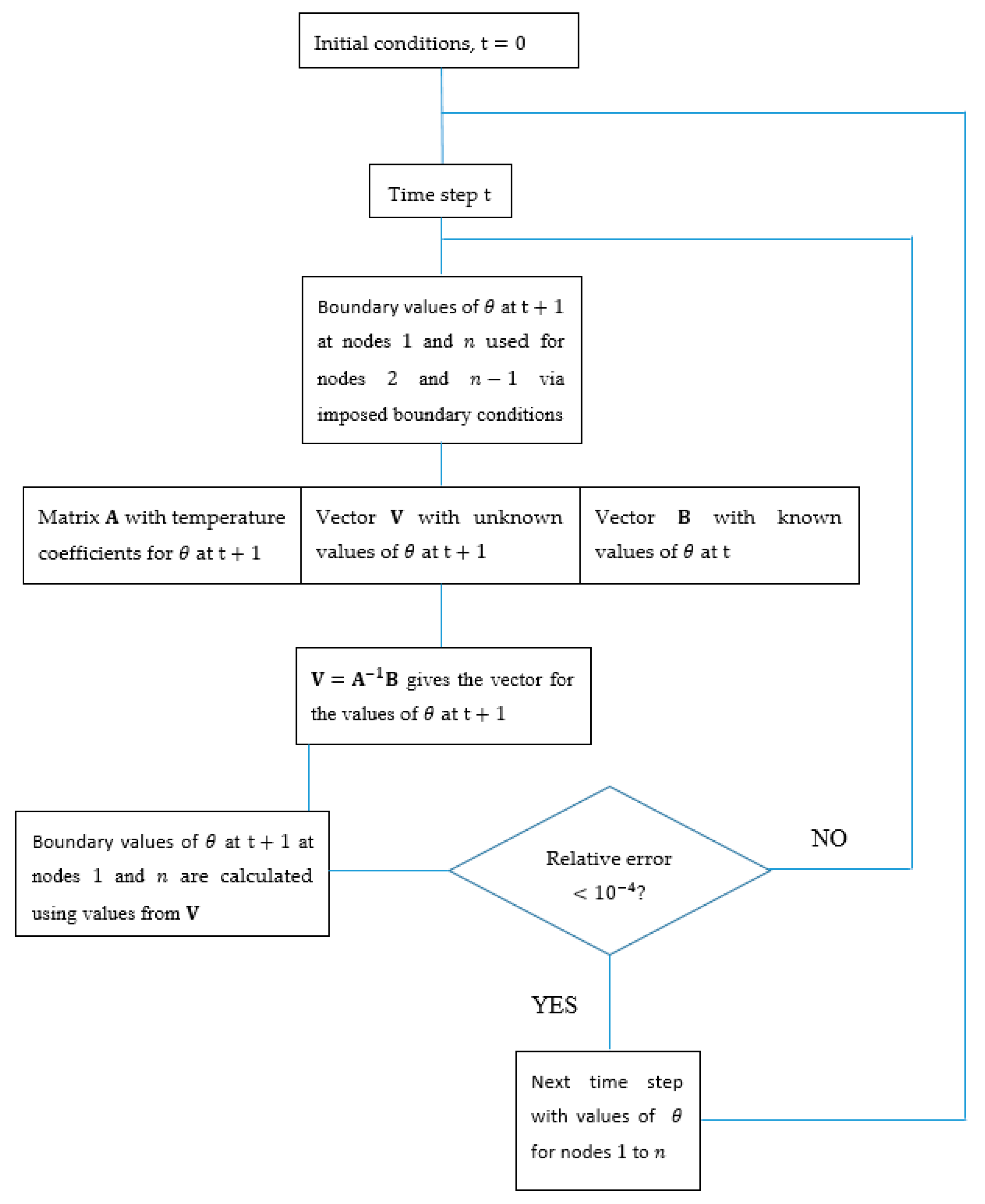
The model is solved by using a semi-implicit difference method for the spatial discretization and the forward Euler method for the temporal discretization for each time step $t^{*}$. At the beginning of the simulation, the initial conditions are imposed. At a certain time $t^{*}$, the equations for the temperatures are written in matrix form, $A\ast V=B$, where $A$ is a matrix of dimension $\left(\mathrm{n}-2\right)\times \left(\mathrm{n}-2\right)$ ($\mathrm{n}$ being the number of nodes in the discretized spatial domain, and two nodes being dedicated to the boundary conditions; the bulk equations are thus discretized on $\left(\mathrm{n}-2\right)$ nodes), containing the coefficients of the temperatures at time $t^{*}+1$, $V$, a vector of dimension $\left(\mathrm{n}-2\right)$ containing the unknown temperature values at the spatial nodes at time $t^{*}+1,$ and $B$ being a vector of dimension $\left(\mathrm{n}-2\right),$ containing the known temperature values at time $t^{*}$. Due to the spatial gradients in the bulk equations, the values at nodes $2$ and $\mathrm{n}-1$ depend on the boundary values at nodes $1$ and $\mathrm{n}$, respectively. The vector $V$ is calculated as $V=A^{-1}B$. The boundary condition for the ballistic temperature at the hot side is imposed and held at that value at each time step. The boundary condition for the ballistic temperature at the cold side as well as the boundary conditions of the diffusive temperature at both sides at time $t^{*}+1$ are then obtained through the bulk values at time $t^{*}+1$. This procedure is repeated until the relative errors of the bulk and boundary values of both the ballistic and diffusive temperatures between the previous and present loops become smaller than ${10}^{-4}$. The obtained values at time $t^{*}+1$ are stocked in the output matrix, and used as the known values for the next time step $t^{*}+2$. This procedure is outlined in a schematic form in Figure 1.

4. Results

4.1. Temperature Distribution of the Two-Temperature Model

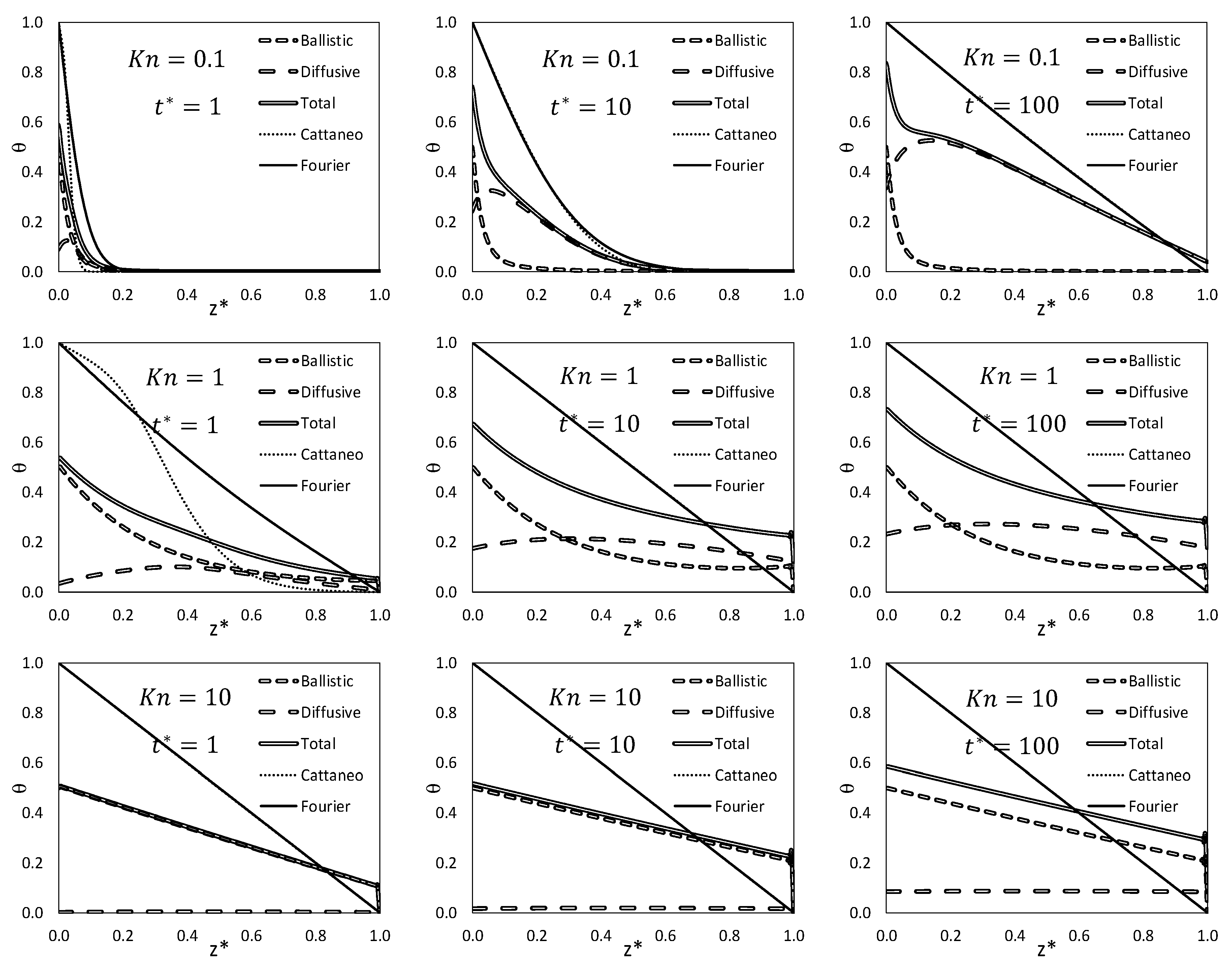
The model described in the previous section has been solved using Mathematica. In Figure 2, the non-dimensional temperature profiles are shown for $K\mathrm{n}=0.1$, $1$ and $10$, where $K{\mathrm{n}}_{\mathrm{d}}=K{\mathrm{n}}_{\mathrm{b}}=K\mathrm{n}$. These values for $K\mathrm{n}$ are chosen, since they all represent cases where both the diffusive and ballistic regimes are present, with a dominant diffusive regime for $K\mathrm{n}=0.1$, and a dominant ballistic one for $K\mathrm{n}=10$. The results are presented for three non-dimensional times: $t^{*}=1$, $10,$ and $100$. In order to emphasize the relative importance of the two contributions in our model, both the ballistic and diffusive components of the temperature are shown next to the non-dimensional temperature (labelled as “Total”). For comparison, the results from Fourier’s and Cattaneo’s models are presented as well. We notice that generally, the region close to the hot side ($z^{*}=0$) is mainly dominated by the ballistic component contribution, which decreases with space, while the diffusive one is increasing up to a maximum (not so discernible for $K\mathrm{n}=10$), after which one observes a decrease. This descent is the steepest for smaller $K\mathrm{n}$. As expected, the influence of the ballistic component becomes more important as $K\mathrm{n}$ is larger, whilst that of the diffusive component is dominant for smaller values of $K\mathrm{n}$. Moreover, although the ballistic component develops earlier, it appears that afterwards, the diffusion component is growing more over time than the ballistic one. This observation reflects the conversion of the ballistic internal energy into the diffusive one in time, but the reverse is not possible. We can also observe that for small $K\mathrm{n}$ values, the temperature at the cold side is close to zero, the reference value. The fact that this temperature for $K\mathrm{n}=0.1$ is not exactly zero, is due to the weak, non-zero, ballistic component that is responsible for well-known temperature jumps. These temperature jumps are more pronounced at larger $K\mathrm{n}$ values, and are clearly seen for $K\mathrm{n}=10$. Finally, it can be seen that Fourier’s and Cattaneo’s laws are qualitatively close to our model for small values of $K\mathrm{n}$ (more dominant diffusive regime), but they differ considerably for larger values of $K\mathrm{n}$ (higher ballistic contribution).

4.2. Temperature Distribution of the Fourier and Cattaneo Laws with an Effective Thermal Conductivity

Another way of studying heat conduction through nanomaterials is to use Fourier’s or Cattaneo’s law, but with an effective thermal conductivity, ${\mathsf{\lambda }}_{\mathrm{eff}}$, that takes into account the size of the material. We propose to write ${\mathsf{\lambda }}_{\mathrm{eff}}$ in the form:

$${\mathsf{\lambda }}_{\mathrm{eff}}={\mathsf{\lambda }\mathrm{f}}_{\mathrm{c}}$$

(34)

where $\mathsf{\lambda }$ stands for the bulk thermal conductivity, and the contributions linked to the size-effects of the nanoparticles are described by the correction factor, ${\mathrm{f}}_{\mathrm{c}}$. To determine ${\mathrm{f}}_{\mathrm{c}}$, it is the idea to upgrade the heat flux and its higher order fluxes to the rank of independent variables at the same footing as the energy or the temperature. This procedure has been presented in Section 2. The strength of this development is that from Equations (8) and (9); not only constitutive equations can be obtained, but they can also be used to propose effective properties. In the case of heat transfer, this concerns effective thermal conductivity. So, continuing from Equations (8) and (9), we present how this can be obtained. The physical meanings of the phenomenological coefficients are also already discussed and obtained in Section 2. We assume now that the system is described by an infinite number of flux variables, i.e., $\mathrm{N}\to \infty$. Applying the spatial Fourier transform $q\left(k,\mathrm{t}\right)={{\displaystyle \int }}_{-\infty }^{+\infty }q\left(r,\mathrm{t}\right){\mathrm{e}}^{-\mathrm{i}k𝓈r}\mathrm{d}r$ to relations (8) and (9), with $k$ as the wave-number vector and $r$ as the position vector, one is led to the following evolution equation of the Fourier-transformed heat flux:

$$\mathsf{\tau }{\mathrm{d}}_{\mathrm{t}}\widehat{q}\left(k\right)+\widehat{q}\left(k\right)=-\mathrm{i}k\mathsf{\lambda }\left(k\right)\widehat{\mathrm{T}}\left(k\right),$$

(35)

where $\mathsf{\lambda }\left(k\right)$ is wavelength-dependent thermal conductivity, taking the form of a continued fraction expansion [24,28,31], so that the correction factor (this continued fraction divided by $\mathsf{\lambda }$) finally becomes:

$${\mathrm{f}}_{\mathrm{c}}\left(k\right)=\frac{1}{1+\frac{k^2{\mathrm{l}}_1^2}{1+\frac{k^2{\mathrm{l}}_2^2}{1+\frac{k^2{\mathrm{l}}_3^2}{1+\dots }}}},$$

(36)

where $l_n$ is the correlation length of order n defined by ${\mathrm{l}}_{\mathrm{n}}^2=\frac{{\mathsf{\beta }}_{\mathrm{n}}^2}{{\mathsf{\nu }}_{\mathrm{n}}{\mathsf{\nu }}_{\mathrm{n}+1}}={\mathcal{l}}^2$, following the discussion under (15). This is reasonable if one wants to obtain constitutive relations, which was the case in Section 3 (even the first order of fluxes is, in most cases, sufficient). Furthermore, it is quite necessary to limit the order of fluxes, so that analytical solutions can be found, or numerical simulations can be performed. However, when one wants to use Fourier’s or Cattaneo’s law, it is necessary to take into account an infinite number of higher-order fluxes in the framework of an effective thermal conductivity. In that case, we need to use kinetic theories [32,33]. In case we consider heat transfer in one direction (such as through thin films), kinetic theories [32,33] stipulate that the correlation lengths should be selected as ${\mathrm{l}}_{\mathrm{n}}^2={\mathrm{a}}_{\mathrm{n}+1}{\mathcal{l}}^2$, with ${\mathrm{a}}_{\mathrm{n}}={\mathrm{n}}^2/\left(4{\mathrm{n}}^2-1\right)$, and $\mathcal{l}$ is identified as the mean free path, independent of the order of approximation. Generally, kinetic theories [32,33] also hold that the relaxation times ${\mathsf{\tau }}_{\mathrm{n}}$ ($\mathrm{n}>1$), corresponding to higher order fluxes, are limited by the first-order one, i.e., ${\mathsf{\tau }}_1$. In the limit of the latter, we take ${\mathsf{\tau }}_{\mathrm{n}}={\mathsf{\tau }}_1=\mathsf{\tau }$. In the case of nanoparticles or nanofilms, there is only one dimension, namely the radius ${\mathrm{a}}_{\mathrm{p},\mathrm{s}}$ of the spheres, or the thickness of the nanofilms. It is therefore natural to define $k=\mathrm{k}\equiv 2\mathsf{\pi }/{\mathrm{a}}_{\mathrm{p},\mathrm{s}}$. With these results in mind, and taking the stationary solution, the continued fraction (34) reduces to an asymptotic limit [32,34], leading finally to the following expression for ${\mathrm{f}}_{\mathrm{c}}$:

$${\mathrm{f}}_{\mathrm{c}}=\frac{3}{4{\mathsf{\pi }}^2{\mathrm{Kn}}^2}\left(\frac{2{\mathsf{\pi }\mathrm{Kn}}_{\mathrm{d}}}{\arctan \left(2{\mathsf{\pi }\mathrm{Kn}}_{\mathrm{d}}\right)}-1\right)$$

(37)

where the Knudsen number is defined as $Kn=\mathcal{l}/{\mathrm{a}}_{\mathrm{p},\mathrm{s}}$. Combining (34) and (37) leads to the effective thermal conductivity:

$${\mathsf{\lambda }}_{\mathrm{eff}}=\frac{3\mathsf{\lambda }}{4{\mathsf{\pi }}^2{\mathrm{Kn}}^2}\left(\frac{2{\mathsf{\pi }\mathrm{Kn}}_{\mathrm{d}}}{\arctan \left(2{\mathsf{\pi }\mathrm{Kn}}_{\mathrm{d}}\right)}-1\right)$$

(38)

With (38) instead of $\mathsf{\lambda }$, we can define effective Fourier and Cattaneo laws. Using these effective laws in combination with (19) with $r=0$, we finally obtain in dimensionless form:

$$\frac{\partial {\mathsf{\theta }}_{\mathrm{f}}}{\partial {\mathrm{t}}^{*}}-\frac{1}{4{\mathsf{\pi }}^2}\left(\frac{2{\mathsf{\pi }\mathrm{Kn}}_{\mathrm{d}}}{\arctan \left(2{\mathsf{\pi }\mathrm{Kn}}_{\mathrm{d}}\right)}-1\right)\frac{{\partial }^2{\mathsf{\theta }}_{\mathrm{f}}}{\partial {\mathrm{z}}^{*}{}^2}=0$$

(39)

$$\frac{{\partial }^2{\mathsf{\theta }}_{\mathrm{c}}}{\partial {\mathrm{t}}^{*}{}^2}+\frac{\partial {\mathsf{\theta }}_{\mathrm{c}}}{\partial {\mathrm{t}}^{*}}-\frac{1}{4{\mathsf{\pi }}^2}\left(\frac{2{\mathsf{\pi }\mathrm{Kn}}_{\mathrm{d}}}{\arctan \left(2{\mathsf{\pi }\mathrm{Kn}}_{\mathrm{d}}\right)}-1\right)\frac{{\partial }^2{\mathsf{\theta }}_{\mathrm{c}}}{\partial {\mathrm{z}}^{*}{}^2}=0$$

(40)

Figure 3 compares the total temperature from our model (from Figure 2) to the ones obtained from (39) and (40).

Figure 3 shows that, although no exact correspondence is observed, for small $Kn$ numbers and large times, the effective Cattaneo and Fourier results are qualitatively not far from our results. The temperature jumps are not represented by these effective models, and for large Kn numbers and small times, even the qualitative comparison does not hold. In general, the effective model, presented in this section, is reasonable for cases where the $Kn$ number is not too high ($Kn\le O\left(1\right)$) and the system is close to stationarity (at large times, moving slowly, and being close to their quasi-stationary state).

5. Discussion

The work started by showing principles, using Extended Non-Equilibrium Thermodynamics, in order to obtain constitutive equations that are applicable to systems at nanoscale. Since the subject of this paper is focused on heat transport, a generalized equation for heat transport is used for the purposes of considering the problem of heat conduction through a rigid nanofilm. The central assumption of the present work is that, contrary to previous approaches, the set of variables, namely the internal energy and the energy flux, is split into contributions of diffusive and ballistic natures. Heat transport is represented here as a two-component diffusion-reaction process, where ballistic particles can convert irreversibly into diffusive ones. The latter are obeying a Cattaneo equation, while the behaviors of the ballistic phonons are dictated by the aforementioned generalized Equation (16) and (22). This choice stems from the premise that non-local effects are dominating in ballistic collisions. Often, Fourier and/or Cattaneo laws are used, and are adapted by effective material properties, in order to take into account the mentioned non-local effects. Not expecting exact correspondence, it is interesting how close such an approach can be to our two-temperature model. An effective thermal conductivity is derived from our theory, and introduced into the Fourier and Cattaneo laws, for the purposes of comparison with our model. The results suggest that the comparison is reasonable for $Kn\le O\left(1\right)$ and large times.

It should be noted that one of the objectives is to demonstrate the versatility of Extended Non-Equilibrium Thermodynamics, proposing relatively simple solutions to delicate and complicated phenomena at the nanoscale level. However, it is noteworthy to mention that questions may be raised about the definitions of diffusive and ballistic temperatures at nanoscales. This is the reason for why in our development, we considered the two temperatures as measures of internal energies. As such, the diffusive and ballistic components are to be viewed as quasi-temperatures that stand for the amount of internal energy that is of either diffusive or ballistic natures. However, the total internal energy is a well-defined property, and it directly representative for the temperature.

Our approach in this work can be extended beyond the linear regime, considering the non-linear contributions of the heat flux. Nonetheless, it should be realized that this formulation forms the necessary framework for further investigations. A set of variables has been defined, but the most appropriate set of variables is not easy to define: should non-linear terms in the heat flux and their higher orders be included as well, and if so, would this contribute significantly to the correct values of the heat flux? Answering this asks for a more complex mathematical formulation that is not too complicated to formulate, but not easy to solve, nor to interpret physically. Finally, the choice of the boundary conditions is still a delicate issue, and calls for more study.

All in all, the present model presents a solid framework of investigations in heat conduction through nanoscopic materials, and it is shown to be applicable to a transient problem of heat conduction through a nanofilm. Other works, based on the theory put forward here, have proven to be validated against other works [25,30,35].

6. Conclusions

The aim of this work is to show how insight can be obtained into the ballistic and diffusive components of phonon heat transport through a nanofilm, by using extended developments from thermodynamic principles. Our model shows good agreement with other sophisticated models in the literature [25,30,35]. The importance of the ballistic and diffusive components depends on the $K\mathrm{n}$ number. For low $K\mathrm{n}$ numbers, the ballistic component is almost absent, and only persists close to the boundary on the hot side of the nanofilm. This is understandable, since the continuous heat flux passing from the heat source into the nanofilm causes a flux of incident phonons, which are transformed irreversibly almost immediately into diffusion ones. For $K\mathrm{n}$ numbers that are higher, these incident phonons evolve further into the nanofilm, and much less is converted into diffusion phonons. This causes completely different temperature profiles. For small $K\mathrm{n}$ numbers, the result is a temperature profile that is close to the ones predicted by the classical laws. For higher $K\mathrm{n}$ numbers, the temperature profiles are completely different from those from the classical Fourier and Cattaneo laws. One may also observe pronounced temperature jumps on both sides of the nanofilm. For comparison, and also because it is used rather often, the classical laws with effective thermal conductivities are also compared to our complete model. It appears that the comparison is rather satisfactory for small $K\mathrm{n}$ numbers, but not at all for higher $K\mathrm{n}$ numbers. Finally, one may state that for higher $K\mathrm{n}$ numbers, it is necessary to use non-local effects, which are explained by our model to come from the ballistic phonons that are only slightly transformed into diffusive ones.

References

- Machrafi, H.; Lebon, G. General constitutive equations of heat transport at small length scales and high frequencies with extension to mass and electrical charge transport. Appl. Math. Lett. 2016, 52, 30–37. [Google Scholar] [CrossRef] [Green Version]
- Hill, T.L. Thermodynamics of Small Systems; Dover: New York, NY, USA, 1994. [Google Scholar]
- Niemann, J.; Härter, S.; Kästle, C.; Franke, J. Challenges of the miniaturization in the electronics production on the example of 01005 components. In Tagungsband des 2. Kongresses Montage Handhabung Industrieroboter; Springer Vieweg: Berlin, Germany, 2017; pp. 113–123. [Google Scholar]
- Moore, A.L.; Shi, L. Emerging challenges and materials for thermal management of electronics. Materialstoday 2014, 17, 163–174. [Google Scholar] [CrossRef]
- Cahill, D.G.; Ford, W.K.; Goodson, K.E.; Mahan, G.D.; Majumdar, A.; Maris, H.J.; Merlin, R.; Phillpot, S.R. Nanoscale thermal transport. J. Appl. Phys. 2003, 93, 793. [Google Scholar] [CrossRef]
- Dinh, T.; Phan, H.P.; Kashaninejad, N.; Nguyen, T.K.; Dao, D.V.; Nguyen, N.T. An on-chip SiC MEMS device with integrated heating, sensing, and microfluidic cooling systems. Adv. Mater. Interfaces 2018, 5, 1800764. [Google Scholar] [CrossRef]
- Zheng, W.; Huang, B.; Li, H.; Koh, Y.K. Achieving huge thermal conductance of metallic nitride on graphene through enhanced elastic and inelastic phonon transmission. ACS Appl. Mater. Interfaces 2018, 10, 35487–35494. [Google Scholar] [CrossRef] [PubMed]
- Yang, L.; Chen, Z.G.; Dargusch, M.S.; Zou, J. High performance thermoelectric materials: Progress and their applications. Adv. Energy Mater. 2018, 8, 1701797. [Google Scholar] [CrossRef]
- Yang, N.; Xu, X.; Zhang, G.; Li, B. Thermal transport in nanostructures. AIP Adv. 2012, 2, 041410. [Google Scholar] [CrossRef] [Green Version]
- Kuleyev, I.I.; Kuleyev, I.G.; Bakharev, S.M. Phonon focusing and features of phonon transport in silicon nanofilms and nanowires at low temperatures. Phys. Status Solidi B 2015, 252, 323–332. [Google Scholar] [CrossRef]
- Terris, D.; Joulain, K.; Lacroix, D.; Lemonnier, D. Numerical simulation of transient phonon heat transfer in silicon nanowires and nanofilms J. Phys. Conf. Ser. 2007, 92, 012077. [Google Scholar] [CrossRef]
- Gao, Y.; Bao, W.; Meng, Q.; Jing, Y.; Song, X. The thermal transport properties of single-crystalline nanowires covered with amorphous shell: A molecular dynamics study. J. Non-Cryst. Solids 2014, 387, 132–138. [Google Scholar] [CrossRef]
- Kaiser, J.; Feng, T.; Maassen, J.; Wang, X.; Ruan, X.; Lundstrom, M. Thermal transport at the nanoscale: A Fourier’s law vs. phonon Boltzmann equation study. J. Appl. Phys. 2017, 121, 044302. [Google Scholar] [CrossRef]
- Guo, Y.; Wang, M. Phonon hydrodynamics for nanoscale heat transport at ordinary temperatures. Phys. Rev. B 2018, 97, 035421. [Google Scholar] [CrossRef]
- Tang, D.S.; Hua, Y.C.; Cao, B.Y. Thermal wave propagation through nanofilms in ballistic-diffusive regime by Monte Carlo simulations. Int. J. Therm. Sci. 2016, 109, 81–89. [Google Scholar] [CrossRef]
- Li, H.L.; Hua, Y.C.; Cao, B.Y. A hybrid phonon Monte Carlo-diffusion method for ballistic-diffusive heat conduction in nano- and micro-structures. Int. J. Heat Mass Transf. 2018, 127, 1014–1022. [Google Scholar] [CrossRef]
- Guyer, R.A.; Krumhansl, J.A. Solution of the linearized Boltzmann phonon equation. Phys. Rev. 1966, 148, 766–778. [Google Scholar] [CrossRef]
- Guyer, R.A.; Krumhansl, J.A. Thermal conductivity, second sound, and phonon hydrodynamic phenomena in nonmetallic Crystals. Phys. Rev. 1966, 148, 778–788. [Google Scholar] [CrossRef]
- Yu, Y.J.; Li, C.L.; Xue, Z.N.; Tian, X.G. The dilemma of hyperbolic heat conduction and its settlement by incorporating spatially nonlocal effect at nanoscale. Phys. Lett. A 2016, 380, 255–261. [Google Scholar] [CrossRef]
- Koh, Y.K.; Cahill, D.G.; Sun, B. Nonlocal theory for heat transport at high frequencies. Phys. Rev. B 2014, 90, 205412. [Google Scholar] [CrossRef]
- Tzou, D.Y. Macro to Microscale Heat Transfer: The Lagging Behaviour; Taylor and Francis: New York, NY, USA, 1997. [Google Scholar]
- Ordonez-Miranda, J.; Alvarado-Gil, J. On the stability of the exact solutions of the dual-phase lagging model of heat conduction. Nanoscale Res. Lett. 2011, 6, 327. [Google Scholar] [CrossRef] [Green Version]
- Cattaneo, C. Sulla conduzione del calore. Atti del Seminario Matematico e Fisico dell’ Universita di Modena 1948, 3, 83–101. [Google Scholar]
- Jou, D.; Casas-Vazquez, J.; Lebon, G. Extended Irreversible Thermodynamics, 4th ed.; Springer: Berlin, Germany, 2010. [Google Scholar]
- Lebon, G.; Machrafi, H.; Grmela, M.; Dubois, C. An extended thermodynamic model of transient heat conduction at sub-continuum scales. Proc. R. Soc. A 2011, 467, 3241–3256. [Google Scholar] [CrossRef] [Green Version]
- Longshaw, S.M.; Borg, M.K.; Ramisetti, S.B.; Zhang, J.; Lockerby, D.A.; Emerson, D.R.; Reese, J.M. mdFoam+: Advanced molecular dynamics in OpenFOAM. Comput. Phys. Commun. 2018, 224, 1–21. [Google Scholar] [CrossRef]
- Machrafi, H. An extended thermodynamic model for size-dependent thermoelectric properties at nanometric scales: Application to nanofilms, nanocomposites and thin nanocomposite films. Appl. Math. Model. 2016, 40, 2143–2160. [Google Scholar] [CrossRef] [Green Version]
- Lebon, G.; Jou, D.; Casas-Vazquez, J. Understanding Non-Equilibrium Thermodynamics; Springer: Berlin, Germany, 2008. [Google Scholar]
- Modest, M.F. Radiative Heat Transfer; McGraw-Hill: New York, NY, USA, 1993. [Google Scholar]
- Alvarez, F.X.; Jou, D. Boundary conditions and Evolution of Ballistic Heat transport. ASME J. Heat Transf. 2010, 132, 0124404. [Google Scholar] [CrossRef]
- Swartz, E.T.; Pohl, R.O. Thermal boundary resistance. Rev. Mod. Phys. 1981, 61, 605–668. [Google Scholar] [CrossRef]
- Hess, S. On Nonlocal Constitutive Relations, Continued Fraction Expansion for the Wave Vector Dependent Diffusion Coefficient. Z. Naturforsch. 1977, 32a, 678–684. [Google Scholar] [CrossRef]
- Machrafi, H. Heat transfer at nanometric scales described by extended irreversible thermodynamics. Commun. Appl. Ind. Math. 2016, 7, 177–195. [Google Scholar] [CrossRef] [Green Version]
- Lebon, G.; Machrafi, H. Effective thermal conductivity of nanostructures: A review. Atti della Accademia Peloritana dei Pericolanti 2019, 96, A14. [Google Scholar] [CrossRef]
- Joshi, A.A.; Majumdar, A. Transient ballistic and diffusive phonon heat transport in thin films. J. Appl. Phys. 1993, 74, 31–39. [Google Scholar] [CrossRef]
Figure 1.
Numerical scheme for . This scheme is general, and applied to all of the temperatures in this study.
Figure 2.
Non-dimensional temperature profiles as a function of distance at different times (, and , respectively) for , , and . The respective contributions of the ballistic, diffusive, and total temperatures are shown and compared to the ones obtained from Cattaneo’s and Fourier’s equations.
Figure 3.
Non-dimensional temperature profiles as a function of distance at different times (, and , respectively) for , , and . The total temperatures from Figure 2 are compared to the ones obtained from Fourier’s and Cattaneo’s equations ((39) and (40)), using the effective thermal conductivity (38).
© 2019 by the author. Licensee MDPI, Basel, Switzerland. This article is an open access article distributed under the terms and conditions of the Creative Commons Attribution (CC BY) license (http://creativecommons.org/licenses/by/4.0/).
Share and Cite
MDPI and ACS Style
Machrafi, H. Temperature Distribution through a Nanofilm by Means of a Ballistic-Diffusive Approach. Inventions 2019, 4, 2. https://doi.org/10.3390/inventions4010002
AMA Style
Machrafi H. Temperature Distribution through a Nanofilm by Means of a Ballistic-Diffusive Approach. Inventions. 2019; 4(1):2. https://doi.org/10.3390/inventions4010002
Chicago/Turabian StyleMachrafi, Hatim. 2019. "Temperature Distribution through a Nanofilm by Means of a Ballistic-Diffusive Approach" Inventions 4, no. 1: 2. https://doi.org/10.3390/inventions4010002