Thermogravitational Cycles: Theoretical Framework and Example of an Electric Thermogravitational Generator Based on Balloon Inflation/Deflation


 , ,
, ,
Abstract
:1. Introduction
2. Materials and Methods
2.1. Theory of Thermogravitational Cycles
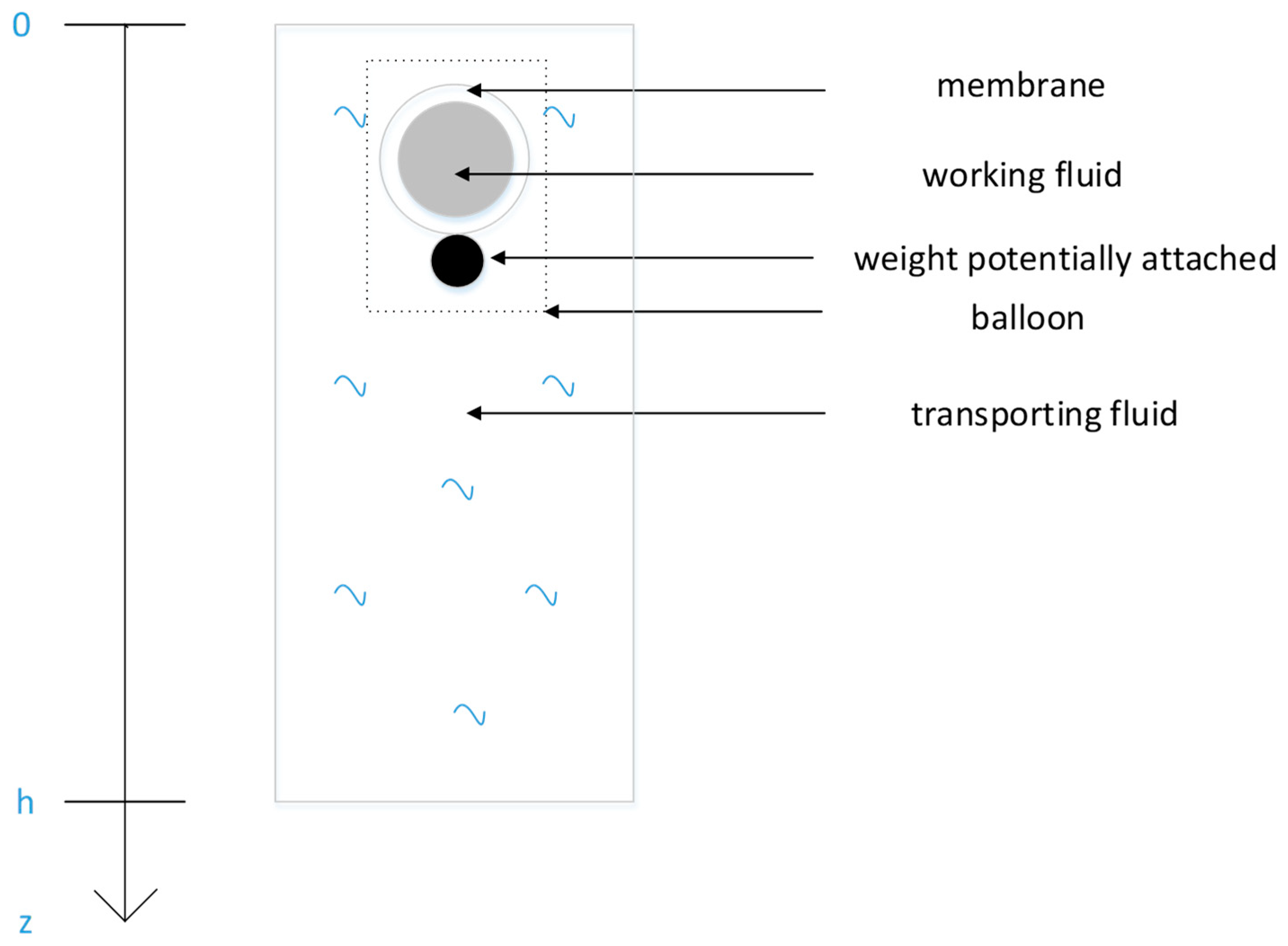
2.1.1. Concepts
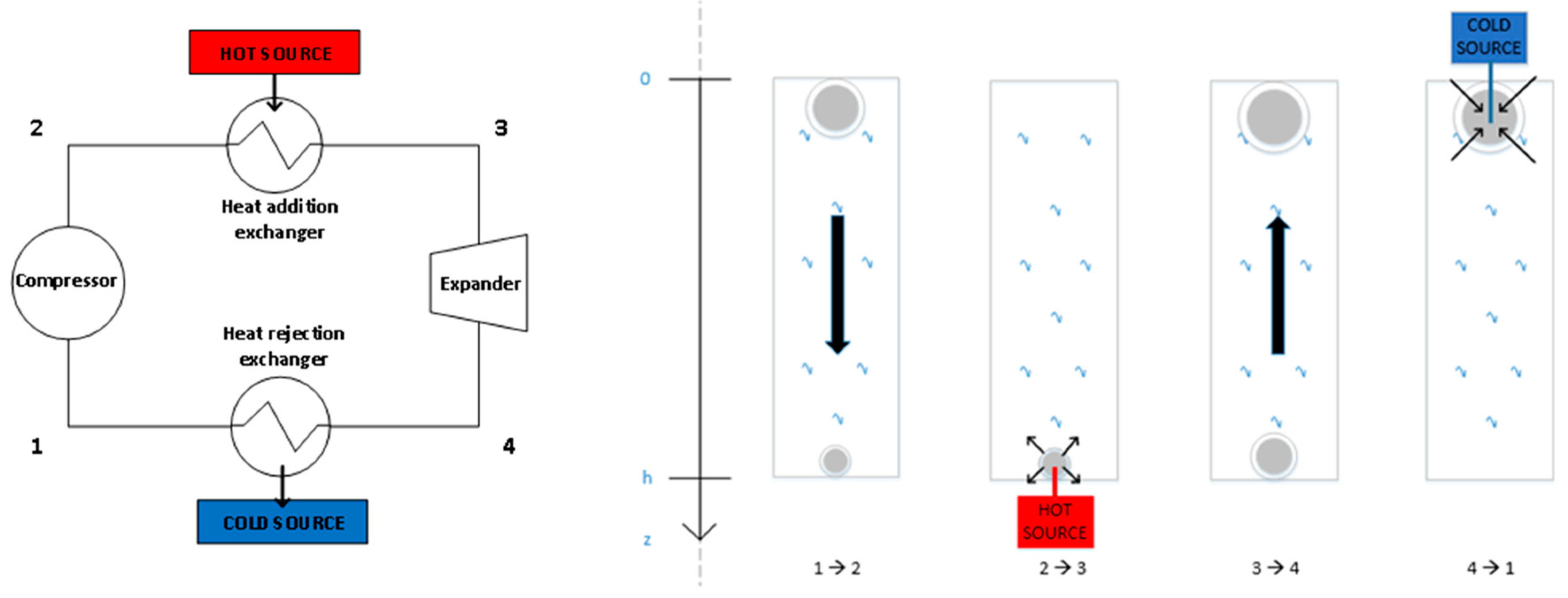
Thermogravitational Power Cycle
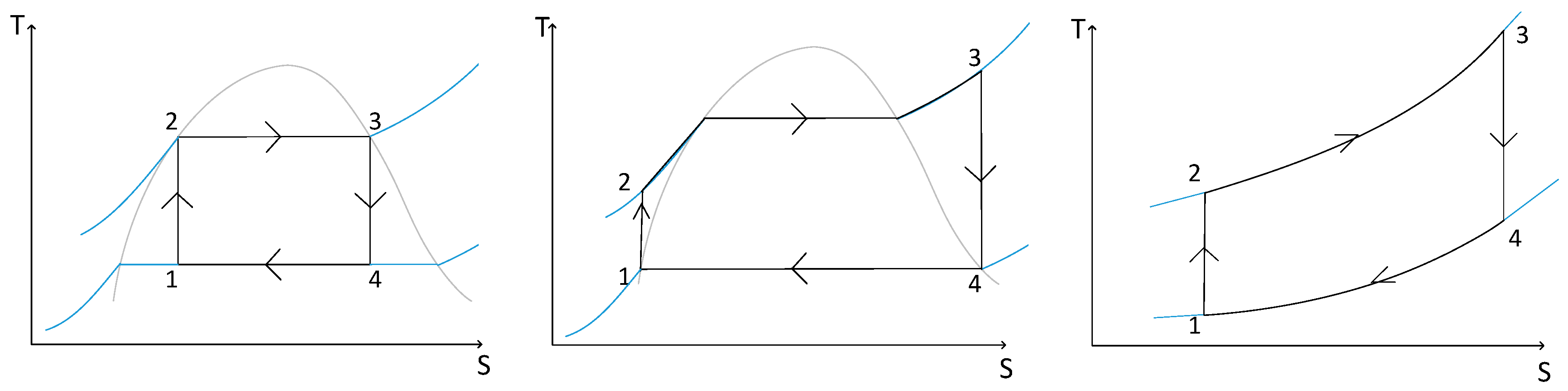
- 1→2: The balloon is originally at the column top. The working fluid is at the cold temperature and at pressure . The balloon falls towards the bottom of the column. The working fluid experiences an adiabatic compression and reaches the pressure and the temperature at the end of the compression when the balloon reaches the bottom.
- 2→3: At the column bottom, the working fluid is put in contact with the hot source at temperature where . The working fluid receives heat from the hot source and experiences an isobaric expansion at pressure .
- 3→4: The balloon rises towards the column top. The working fluid experiences an adiabatic expansion and reaches the pressure and the temperature at the end of the expansion when the balloon reaches the top.
- 4→1: At the column top, the working fluid is put in contact with the cold source at temperature where . The working fluid passes heat to the cold source and experiences an isobaric compression at pressure .
Thermogravitational Pure Power Cycle
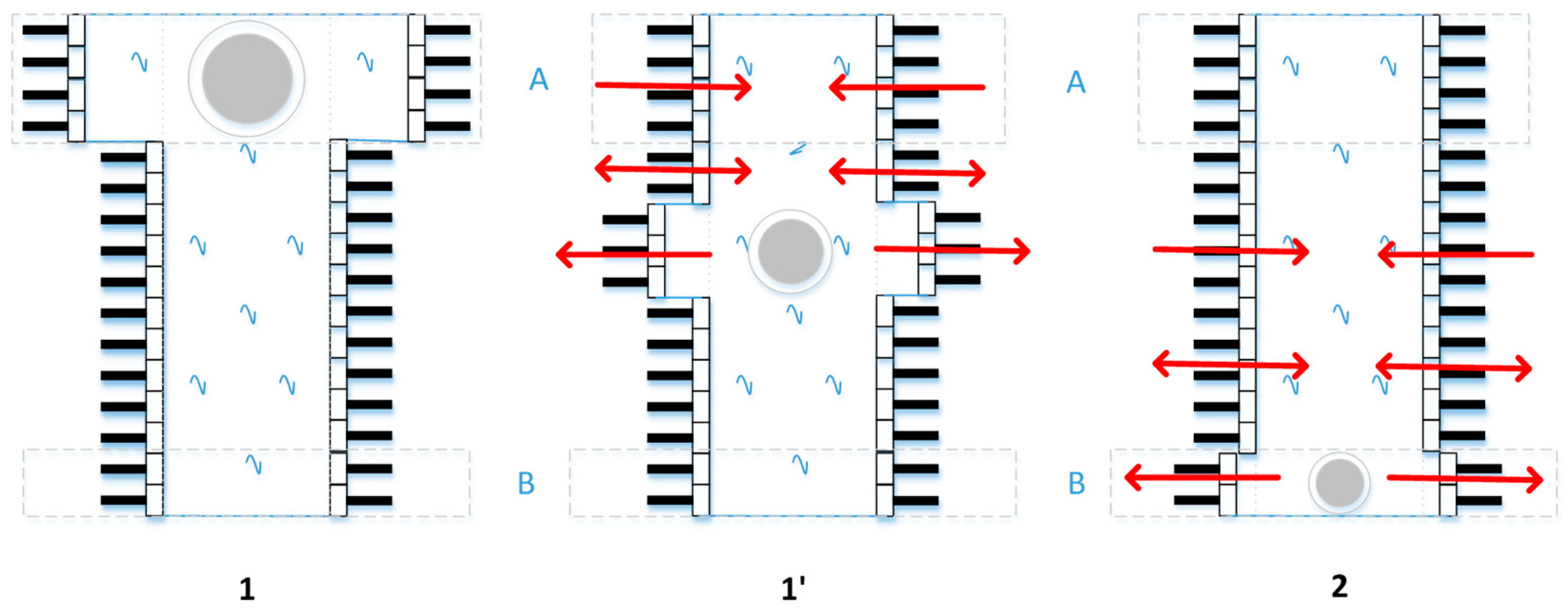
2.1.2. Side Piston Concept
- 1: the balloon has been inserted at the top of the column which was originally totally filled with the transporting fluid and the top pistons of the sub-system A have been displaced in order to accommodate the balloon volume.
- 1′: the balloon has left the top of the column and the top pistons of the sub-system A move inwards by receiving a work input.
- 2: the balloon has reached the bottom of the column. The bottom pistons of the sub-system B are displaced outwards, delivering a work output, in order to accommodate the balloon volume.
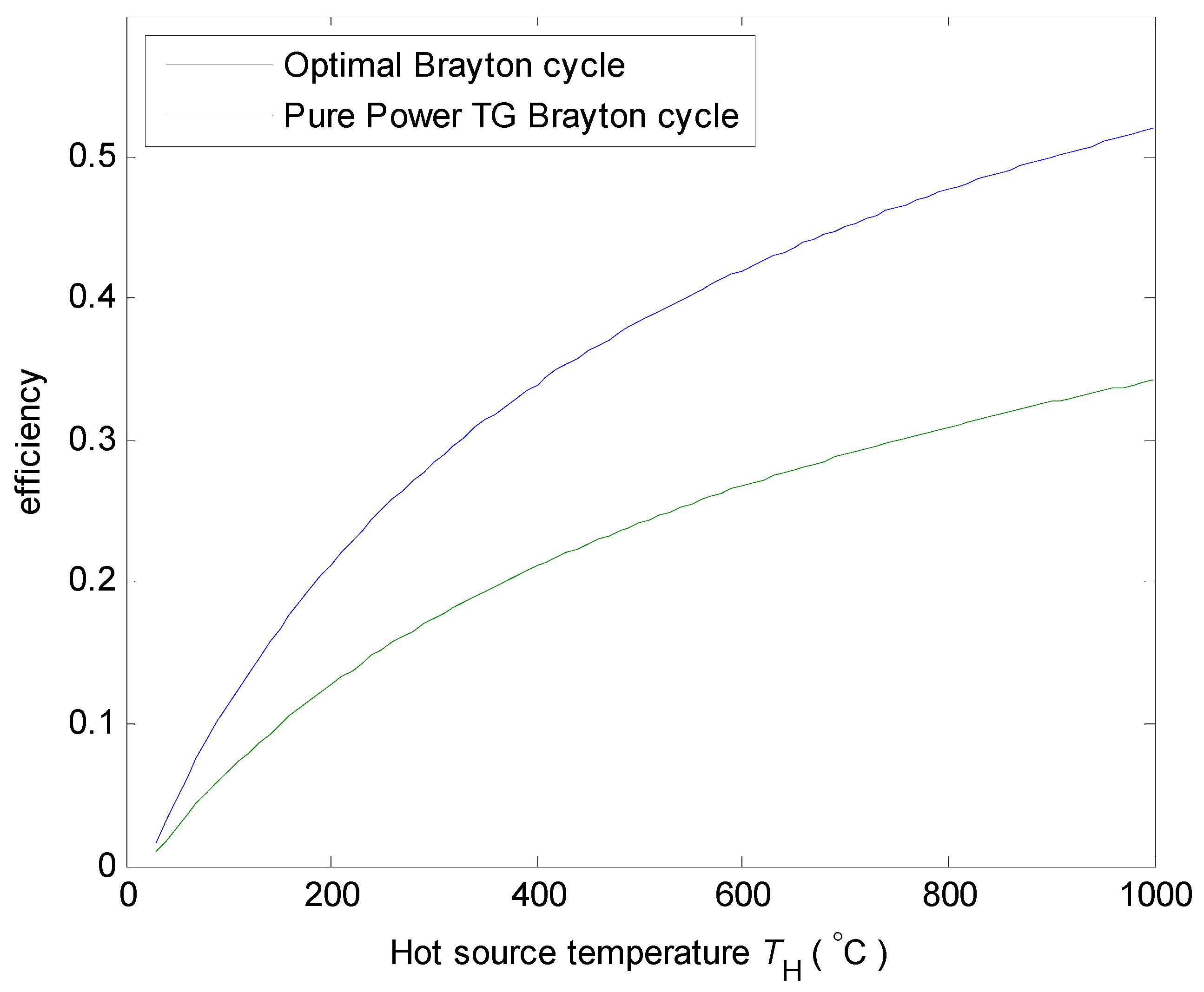
2.1.3. Ideal Thermogravitational Power Cycles
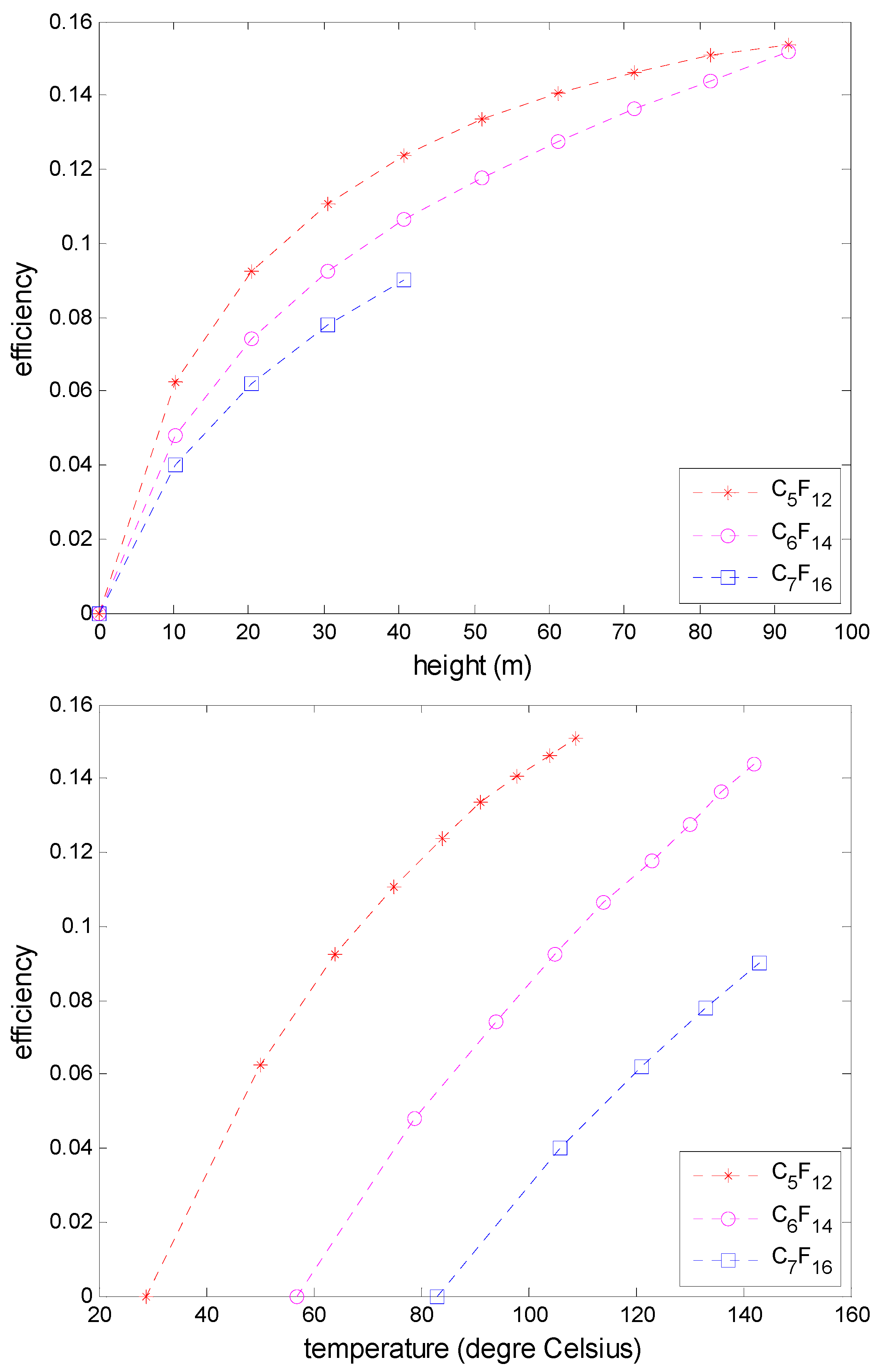
Thermogravitational Power Cycle Efficiency
Thermogravitational Phase-Change Cycles
Thermogravitational Gas Cycle
2.2. Thermogravitational Electric Generator
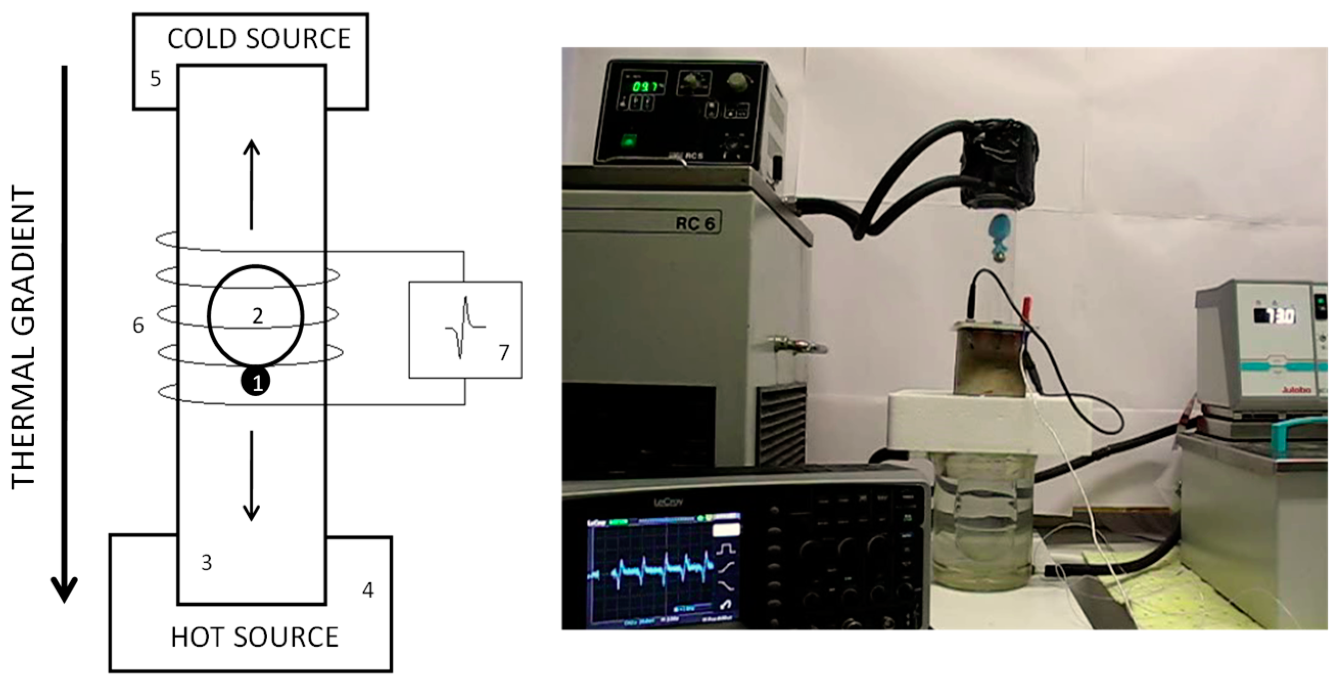
2.2.1. Experiment
2.2.2. Electrical and Mechanical Analysis
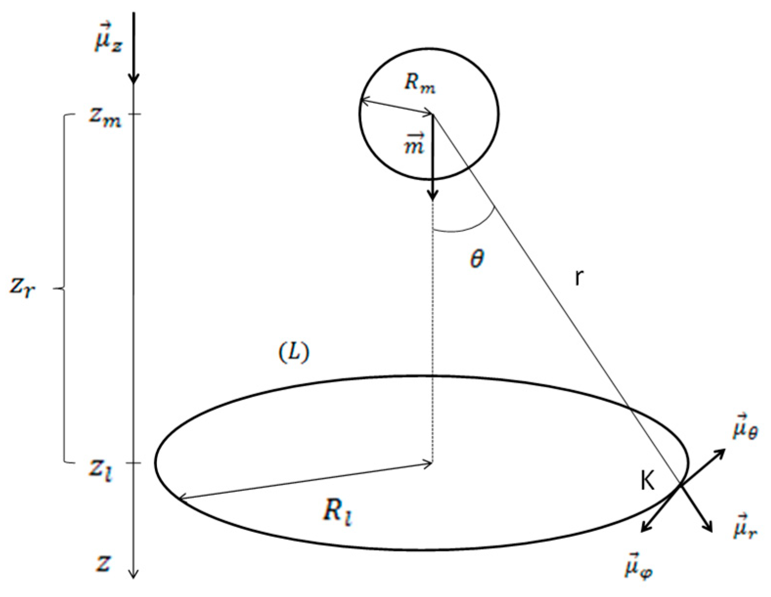
Electromotive Force Calculation
Magnetic Marble Speed and Position
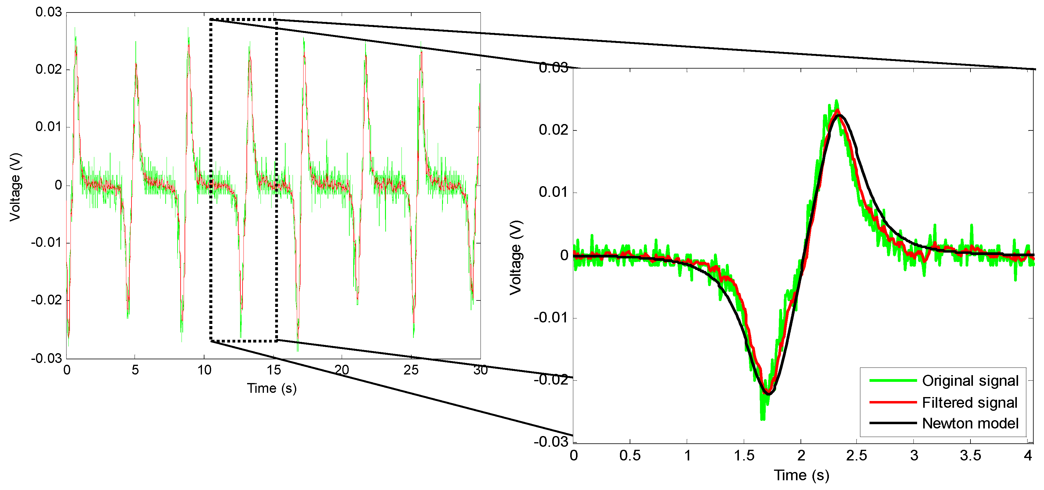
3. Results
4. Discussion
5. Conclusions
6. Patents
Supplementary Materials
Author Contributions
Funding
Acknowledgments
Conflicts of Interest
References
- Heap, R.D. Heat Pumps; E. & F. N. Spon Ltd.: London, UK, 1979. [Google Scholar]
- Hung, T.C.; Shai, T.Y.; Wang, S.K. A review of organic Rankine cycles (ORCs) for the recovery of low-grade waste heat. Energy 1997, 22, 661–667. [Google Scholar] [CrossRef]
- Borsukiewicz-Gozdur, A.; Nowak, W. Comparative analysis of natural and synthetic refrigerants in application to low temperature Clausius–Rankine cycle. Energy 2007, 32, 344–352. [Google Scholar] [CrossRef]
- Saleh, B.; Koglbauer, G.; Wendland, M.; Fischer, J. Working fluids for low-temperature organic Rankine cycles. Energy 2007, 32, 1210–1221. [Google Scholar] [CrossRef]
- Schuster, A.; Karellas, S.; Kakaras, E.; Spliethoff, H. Energetic and economic investigation of Organic Rankine Cycle applications. Appl. Therm. Eng. 2009, 29, 1809–1817. [Google Scholar] [CrossRef] [Green Version]
- Walsh, C.; Thornley, P. A comparison of two low grade heat recovery options. Appl. Therm. Eng. 2013, 53, 210–216. [Google Scholar] [CrossRef] [Green Version]
- Rhinefrank, K.; Agamloh, E.B.; von Jouanne, A.; Wallace, A.K.; Prudell, J.; Kimble, K.; Aills, J.; Schmidt, E.; Chan, P.; Sweeny, B.; et al. Novel ocean energy permanent magnet linear generator buoy. Renew. Energy 2006, 31, 1279–1298. [Google Scholar] [CrossRef]
- Etemadi, A.; Emdadi, A.; AsefAfshar, O.; Emami, Y. Electricity generation by the ocean thermal energy. Energy Procedia 2011, 12, 936–943. [Google Scholar] [CrossRef]
- Du, Y.P.; Ding, Y.L. Feasibility of small-scale cold energy storage (CES) through carbon dioxide based Rankine cycle. J. Energy Storage 2016, 6, 40–49. [Google Scholar] [CrossRef]
- Leijon, M.; Danielsson, O.; Eriksson, M.; Thorburn, K.; Bernhoff, H.; Isberg, J.; Sundberg, J.; Ivanova, I.; Sjöstedt, E.; Ågren, O.; et al. An electrical approach to wave energy conversion. Renew. Energy 2006, 31, 1309–1319. [Google Scholar] [CrossRef]
- Thorburn, K.; Bernhoff, H.; Leijon, M. Wave energy transmission system concepts for linear generator arrays. Ocean Eng. 2004, 31, 1339–1349. [Google Scholar] [CrossRef]
- Grena, R. Energy from solar balloons. Sol. Energy 2010, 84, 650–665. [Google Scholar] [CrossRef]
- Edmonds, I. Hot air balloon engine. Renew. Energy 2009, 34, 1100–1105. [Google Scholar] [CrossRef]
- Flament, C.; Houillot, L.; Bacri, J.-C.; Browaeys, J. Voltage generator using a magnetic fluid. Eur. J. Phys. 2000, 21, 145–149. [Google Scholar] [CrossRef]
- Schoenmaker, J.; Rey, J.F.Q.; Pirota, K.R. Buoyancy organic Rankine cycle. Renew. Energy 2011, 36, 999–1002. [Google Scholar] [CrossRef]
- Li, J.; Pei, G.; Li, Y.; Ji, J. Analysis of a novel gravity driven organic Rankine cycle for small-scale cogeneration applications. Appl. Energy 2013, 108, 34–44. [Google Scholar] [CrossRef]
- Moran, M.J.; Shapiro, H.N. Fundamentals of Engineering Thermodynamics, 6th ed.; John Wiley & Sons Ltd.: West Sussex, UK, 2008. [Google Scholar]
- CHEMCAD Chemstations. P & I Design Limited, Thornaby, Cleveland, UK. Available online: https://www.chemcad.co.uk (accessed on 29 November 2018).
- AIChE. Design Institute for Physical Properties. Available online: https://www.aiche.org/dippr (accessed on 29 November 2018).
- Edwards, J.E. Process Modelling Selection of Thermodynamic Methods. 2008. Available online: https://www.pidesign.co.uk/ (accessed on 22 November 2018).
- Balmer, R.T. Modern Engineering Thermodynamics; Elsevier: Amsterdam, The Netherlands, 2011. [Google Scholar]
- Product Information Fluorinert™ FC-72, 3M™ 2000. Available online: http://multimedia.3m.com/mws/media/64892O/fluorinert-electronic-liquid-fc-72.pdf (accessed on 22 November 2018).
- Kao, C.-P.C.; Sievert, A.C.; Schiller, M.; Sturgis, J.F. Double azeotropy in binary mixtures 1,1,1,2,3,4,4,5,5,5-decafluoropentane high-boiling diastereomer + tetrahydrofuran. J. Chem. Eng. Data 2004, 49, 532–536. [Google Scholar] [CrossRef]
- Reitz, J.R.; Milford, F.J.; Christy, R.W. Foundations of Electromagnetic Theory, 4th ed.; Addison-Wesley Publishing Company: Boston, MA, USA, 2008. [Google Scholar]
- Bashtovoi, V.G.; Reks, A.G. Electromagnetic induction phenomena for a nonmagnetic non-electroconducting solid sphere moving in a magnetic fluid. J. Magn. Magn. Mater. 1995, 149, 84–86. [Google Scholar] [CrossRef]
- White, F.M. Fluid Mechanics, 3rd ed.; McGraw-Hill Education: New York, NY, USA, 1994. [Google Scholar]
- Timmerman, P.; van der Weele, J.P. On the rise and fall of a ball with linear or quadratic drag. Am. J. Phys. 1999, 67, 538–546. [Google Scholar] [CrossRef]
- Aouane, K. Thermogravitational Cycles. MSc Thesis, Department of Mechanical Engineering, University College London, London, UK, 2014. [Google Scholar]
- Ozone Secretariat United Nations Environment Programme. The Montreal Protocol on Substances That Deplete the Ozone Layer; United Nations Environment Programme: Nairobi, Kenya, 2000. [Google Scholar]
- United Nations Framework Convention on Climate Change. Kyoto Protocol to the United Nations Framework Convention on Climate Change; United Nations Framework Convention on Climate Change: Kyoto, Japan, 1997. [Google Scholar]
- European Parliament. Regulation (EC) No. 842/2006 of the European Parliament and of the Council of 17 May 2006 on Certain Fluorinated Greenhouse Gases; European Parliament: Strasbourg, France, 2006. [Google Scholar]


| Disadvantages | Advantages |
|---|---|
| System is not compact: Tall columns | Possibility of wet compression/expansion to approach the Carnot efficiency |
Slow gravitational compression and expansion:
| Can operate even under very low hot source temperature, according to the specifications of the organic fluid used |
| Achieving efficient heat exchanges at the top and bottom of the column could be challenging | Possibility to have pure power cycles |
© 2018 by the authors. Licensee MDPI, Basel, Switzerland. This article is an open access article distributed under the terms and conditions of the Creative Commons Attribution (CC BY) license (http://creativecommons.org/licenses/by/4.0/).
Share and Cite
Aouane, K.; Sandre, O.; Ford, I.J.; Elson, T.P.; Nightingale, C. Thermogravitational Cycles: Theoretical Framework and Example of an Electric Thermogravitational Generator Based on Balloon Inflation/Deflation. Inventions 2018, 3, 79. https://doi.org/10.3390/inventions3040079
Aouane K, Sandre O, Ford IJ, Elson TP, Nightingale C. Thermogravitational Cycles: Theoretical Framework and Example of an Electric Thermogravitational Generator Based on Balloon Inflation/Deflation. Inventions. 2018; 3(4):79. https://doi.org/10.3390/inventions3040079
Chicago/Turabian StyleAouane, Kamel, Olivier Sandre, Ian J. Ford, Tim P. Elson, and Chris Nightingale. 2018. "Thermogravitational Cycles: Theoretical Framework and Example of an Electric Thermogravitational Generator Based on Balloon Inflation/Deflation" Inventions 3, no. 4: 79. https://doi.org/10.3390/inventions3040079