1. Introduction
Since the publication of Nakamoto’s paper in 2008 [
1], the blockchain has attracted increasing interest, both in industry and academia. Defined as a distributed ledger shared between peers, the blockchain is now one of the most discussed topics in many research areas, such as telecommunications, economics, and cryptography. Bitcoin was one of the first protocols leveraging the blockchain to allow theoretically secure transactions between nodes. These transactions are included into blocks and, to append a block to the blockchain, a user needs to solve a computationally intensive task called Proof of Work (PoW) that consists of finding a hash for the desired block that satisfies some constraints. Blocks are chained together by inserting into these a reference to the previous one. The difficulty of the PoW increases over time and is dynamically adjusted to have approximately 1 block appended to the blockchain every 10 minutes. This, on the one hand, is a mechanism that reduces the probability of tampering since, to modify the content of a block, a user needs to provide a new PoW for all the blocks between the modified one and the last discovered block. On the other hand, the PoW is one of the main bottlenecks for the scalability of Bitcoin (and, in general, blockchains based on PoW). To handle an increasing number of transactions, several solutions have been proposed, such as the adoption of different mechanisms not based on PoW [
2]. One of these alternative approaches is the Lightning Network (LN) [
3]: with LN, users create a new layer on top of an existing blockchain where payments can be quickly executed by opening payment channels, locking some funds in and utilizing these funds for the transactions. One of the key features of LN channels is that, from the outside, only the total balance of a channel is known, and not the balance available at the two ends. This is a feature introduced to increase the security of the network. Payments can also travel from two nodes not directly connected by edges, through multi-hop payments. The unknown distribution of a channel’s funds makes the problem of path finding probabilistic: the presence of a path between two nodes does not imply that a payment of a certain size can be successfully routed through it.
Probabilistic Logic Programming (PLP) [
4,
5] is a powerful formalism to represent domains with uncertain relations while retaining all the expressive power of LP, and it has been already applied to solve many different tasks, also in the context of the blockchain [
6]. The structure induced by the LN can be considered as a graph. Logic-based languages are particularly effective in representing relational data and graph structures in general. Moreover, PLP it is a well studied research field with a lot of different available inference algorithms whose correctness has been deeply analysed [
7]. For this reason, PLP is a perfect candidate to model the LN.
In this paper, we show how to leverage PLP and its recently published extensions to model the LN to compute several properties (all the models are available at:
https://bitbucket.org/machinelearningunife/ln_plp_models/src/master/, accessed 1 June 2022). With PLP it is possible, with a simple representation, to compute the probability that a payment came from a certain path or to select the optimal node placement and fund distributions to maximize the routing probability. All these models can also provide considerations regarding the security and the anonymity of the payments. The main goal of the paper is to introduce different models and discuss how they can be applied in the context of LN, and not to provide considerations on its overall structure and topology, as this has already been considered in related works [
8,
9,
10]. To test our approaches, we run some experiments on synthetic datasets that mimic the LN structure with the capacity of the channels chosen from a snapshot of the real LN.
The paper is structured as follows:
Section 2 discusses related work and
Section 3 introduces the basic concepts regarding the blockchain and the Lightning Network.
Section 4 provides an overview of Logic Programming, Probabilistic Logic Programming, and its extensions, which are applied to develop the models discussed in
Section 5. We tested the models and discuss some obtainable information in
Section 6.
Section 7 provides some final remarks and concludes the paper.
2. Related Work
There are several related works in the context of Lightning Network analysis. In [
8], the authors provide a topological analysis of the LN, identify some features such as the average shortest path between two nodes and the degree distribution, and study its robustness in case of edges or node removal. Similar considerations can be found in [
9,
10].
Several attack vectors driven by nodes and edges configurations have been analysed: in [
11], the authors studied a Denial of Service attack based on the LN routing mechanism; in [
12], the authors show the vulnerability of the LN in the case of balance lockdown (“lockdown attack”), where the funds in some edges are blocked in multi hop payments, completely freezing some nodes.
In [
13], the authors discuss how nodes anonymity is affected by the routing mechanism, and, in [
14], the authors analyse how multiple payment attempts can disclose the balance distribution of an edge.
The authors of [
15] propose a probabilistic model of the LN where each edge has an associated probability and discuss the path success probability associated with a payment. Here, we extend this model by considering, differently from [
15], multiple models to compute the probability that at least one path exists between two nodes.
Logic Programming and Probabilistic Logic Programming have already been adopted to model the LN. In [
16], the authors introduced a deterministic model, so not considering uncertainty on the nodes. This model has been extended in [
17], where the authors introduced uncertainty on the distribution of funds. The authors of [
16,
17] propose a Logic and a Probabilistic Logic model of the LN: we extend these models, also by applying new formalism, such as PRLP, POLP, and PALP, to handle an extended class of queries and tasks.
In [
18], the authors represent the LN with a percolation process [
19] and discuss the possible parameters that may influence its structure. They mainly focus on the structure of the network to describe whether a new edge will be added between two nodes, and consider deterministic connections (i.e., two nodes are connected if there is a path). We differ from this work because our focus is on the routing process and we consider probabilistic paths (with a probability dependent on the payment size). In [
20], the authors study LN transaction fees (fee base and fee rate) and suppose that the sender always selects the cheapest route. We do not include transaction fees in our models, but we consider multiple paths in our simulations. Moreover, our focus is on routing while their focus is on the study of the transaction fees and the economic incentives for the nodes. Finally, the authors of [
21] develop different mathematical models to study routing process and propose a novel routing algorithm. We differ from this work because we leverage existing tools to study the routing and do not propose new algorithms. Rather, our goal is to provide tools to extract possible information from the network.
3. Blockchain and Lightning Network
The blockchain can be considered as a distributed ledger composed of blocks chained by cryptographic functions. Every user controls one or more address, each one associated with a public-private key pair, needed to sign transactions and collect funds. Each address can store funds in the form of bitcoin (or fraction of it). Users can send transactions to other users. These typically involve a movement of funds from one or more source addresses to one or more destination addresses. Transactions are gathered by miners and inserted into a block. Each transaction has an associated fee that is collected as a reward by the miner that includes it into a block successfully appended to the blockchain. Every block also contains a reference to the previous one. In the case of Bitcoin, to append a block to the blockchain, a user must provide a solution to a computationally intensive task called Proof of Work (PoW). To solve the PoW, a user must provide a hash for a block that is smaller than a target value. Currently, this problem can only be solved through brute forcing, i.e., trying all possible hashes until a valid one is found, so it is a very challenging task. However, the effective validity of a hash is easy to check. Thanks to the chain of blocks that is created by adding blocks to the blockchain, if a malicious user wants to rewrite the content of a block, he/she needs to provide a PoW for all the next blocks up to the last discovered.
To keep the number of discovered blocks approximately constant over time, the target value is dynamically adjusted. This is a hardcoded specification, and it is one of the main limitations to scalability. Moreover, users need to wait some time before seeing their transactions included into a block since it is not guaranteed that the last executed transactions are the ones that will be included in the next block. Furthermore, due to the possibility of double spending attacks [
22], users wait for some confirmation blocks built on top of the one containing the transaction of interest.
Another factor that limits the number of manageable transactions per second is the maximum block size, set to 1Mb (
https://en.bitcoin.it/wiki/Scalability_FAQ, accessed 1 June 2022). In addition, this is a value hardcoded into the software running the Bitcoin blockchain, so it is unlikely that it will be changed in the future since it will require a backward incompatible update, and the effective benefits are still not truly clear (
https://en.bitcoin.it/wiki/Block_size_limit_controversy, accessed 1 June 2022).
Several solutions have been proposed during the years to alleviate the scalability problem: the first was Segregated Witnesses, which moved some of the information stored into a transaction out of it and introduced the concept of Virtual Size and block weight associated with a transaction. Another proposal, currently under discussion, is the adoption of Schnorr signatures [
23,
24] that will allow for aggregating the signatures required for transactions with multiple inputs controlled by the same user.
An alternative approach is given by “Layer 2” solutions, such as the Lightning Network.
Lightning Network
The Lightning Network (LN) [
3] is a “Layer 2” solution that allows for the creation of a network of peers above an underlying blockchain that supports the processing of quick payments between users. It can be theoretically implemented on top of every blockchain, but here we focus on Bitcoin. The LN works as follows: a couple of users open a bidirectional payment channel between them, through a “commitment transaction” published on the blockchain. Every channel has a certain amount of funds locked in, and this value determines its capacity. The amount of funds in a channel constitutes its balance. In the LN, we consider balances associated with edges, not nodes. Once the channel is created, users can send payments to other users without interacting with the blockchain. In this way, payments can quickly be sent between nodes, and transaction fees are not needed (however, in some cases, small fees are still required to forward a payment in the LN). Once users terminate their operations, they can close the payment channel through a “closing transaction” on the underlying blockchain that updates the balances of the two involved parties to reflect the state of the channel. The LN provides several mechanisms, such as Hashed Timelock Contracts (HTLCs) (
https://en.bitcoin.it/wiki/Hash_Time_Locked_Contracts, accessed 1 June 2022) to manage uncooperative parties.
A key property of the LN is that it allows routing payments between nodes not directly connected by a payment channel. If a node A is connected to a node B, and node B is connected to node C, A can send a multi-hop payment to C, with B forwarding to C the payment received from A. In this case, B collects some fees, composed of a fixed part (base fee) and a variable part (fee rate) that depends on the size of the payment. Thus, the more payments a node routes, the higher will be its earnings. There can be an arbitrary number of intermediate nodes. In addition, here HTLCs manage scenarios where an intermediate node refuses to forward a payment.
Another feature, introduced to increase the security and the anonymity of the users, is that the distribution of funds in a channel is unknown. That is, from the outside, only the total capacity of a channel is available, and not the distribution of funds at the two ends. Consider the following scenario: a user A opens a channel with B and A locks in 5 and B 2 satoshi, where 1 satoshi = bitcoin (These are very small quantities that are unlikely to be realistic but are used here only to explain the process); the total capacity of the channel visible from the outside is , but, from A, we can route towards B at most 5 satoshi, while from B we can route at most 2 satoshi towards A. After, for example, a payment of size 4 from A to B, the total capacity of the channel is unchanged, but the funds distribution is updated: A has 1 satoshi left while B has 6.
The uncertainty of the balance distribution of the channels makes the routing of multi-hop payments difficult since a user needs to try different paths until it succeeds. However, this trial and error process may leak information about the channel distributions, weakening the anonymity property and leading to possible attacks [
14]. For these reasons, the routing problem in the LN can be considered as a probabilistic problem. In the next sections, we discuss how the LN can be encoded using (Probabilistic) Logic Programming models, and we apply several techniques to study the routing process, to compute different probability values, and to reason about possible privacy and security issues.
4. Logic Programming Languages
Here, we introduce the basic concepts needed to understand the models we propose in the next section.
4.1. Logic Programming
Logic Programming (LP), initially proposed in 1974 [
25], is a powerful formalism to represent domains characterized by complex relationships among the involved entities. Prolog [
26] is one of the most famous languages. The basic elements of a Prolog program are
atoms,
terms, and
clauses. Each clause is composed by a
head (an atom) and a
body (a conjunction of atoms or negated atoms, called
literals) separated by the
neck operator (denoted with
:-). The meaning of a clause is: if the body is true, the head is also true. Variables start with uppercase letters while constants start with lowercase letters. With the symbol
_, we denote the anonymous variable, i.e., a variable with no name. If a term or clause does not contain variables, we call it
ground. The operation that consists of replacing variables with terms is called
substitution and it is usually indicated with the Greek letter
. A substitution that makes a term ground is called
grounding. If we consider a term
t(A,B), and a substitution
=
A/a,B/b indicating that we replace
A with
a and
B with
b, the result of the application of
to
t(A,B), denoted with
t, is
t =
t(a,b). In this case, the substitution
is also grounding since the term, after applying the substitution, does not contain variables.
To clarify the previously introduced concepts, consider the program
The first line contains the atom f(a,b), where a and b are terms. Here, f(a,b) can be considered as a fact since it indicates what is known to be true. The second line represents a clause where the head is q(A) and the body is f(A,b). The number of arguments of a term is called arity. The functor of a term is the combination of the name and the number of arguments, often compactly indicated with the notation name/arity. For this example, the two terms can be indicated with f/2 and q/1. A predicate is a set of clauses with the same functor.
To check whether a formula is true or false, we can ask a Prolog interpreter a goal that we also call query. In the previous example, we can ask the Prolog interpreter whether q(A) is true. The answer will be yes with the substitution A = a. The basic mechanism adopted in Prolog to answer queries is called SLD resolution.
We touched here only the surface of LP; for a complete treatment of the field, see [
27,
28].
Consider now a more involved scenario, as described in Example 1.
Example 1 (Deterministic Path).
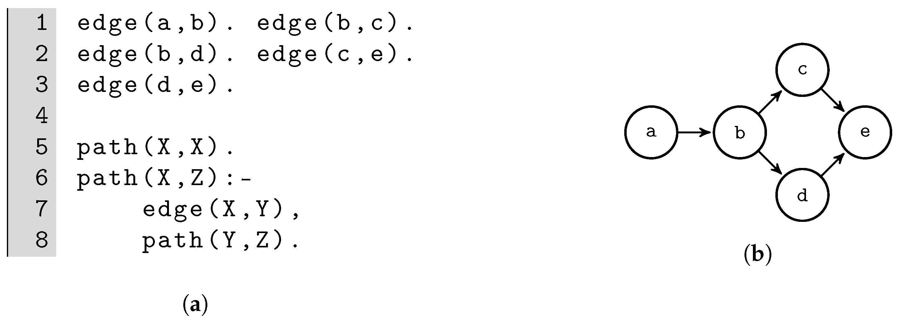
We can represent a network (graph) using a set of edge/2 facts, as shown in Figure 1a. The first rule of Figure 1a (line 5) states that there is certainly a path between X and X (the source and destination nodes coincide). The second rule (line 6) states that there is a path between X and Z if there is an edge between X and an intermediate node Y and there is a path between Y and Z. For this example, the graph does not contain closed loops and edges are directed. We can ask whether there is a path between node a and node e with the query path(a,e). The answer will be yes twice: the first path passes from node c and the second from node d. Alternatively, we can collect all the possible reachable nodes starting from a by asking path(a,X). In this case, the solutions will be X = a, X = b, X = c, X = e, X = d, X = e. Node e is present twice since it can be reachable from two different paths, as previously shown. Logic Programming, despite its expressive power, cannot deal with uncertain data. In this case, we need to adopt Probabilistic Logic Programming (PLP) that we discuss next.
4.2. Probabilistic Logic Programming
Probabilistic Logic Programming (PLP) [
4,
5] extends Logic Programming by considering uncertain information represented as
probabilistic facts. There are several existing languages such as ProbLog [
29], LPAD [
30], and PRISM [
31].
A probabilistic fact
f can be represented using either one of the two following syntaxes:
where
f is an atom and
represents its probability. The notation
is the one adopted in ProbLog [
29] while
is used in LPADs [
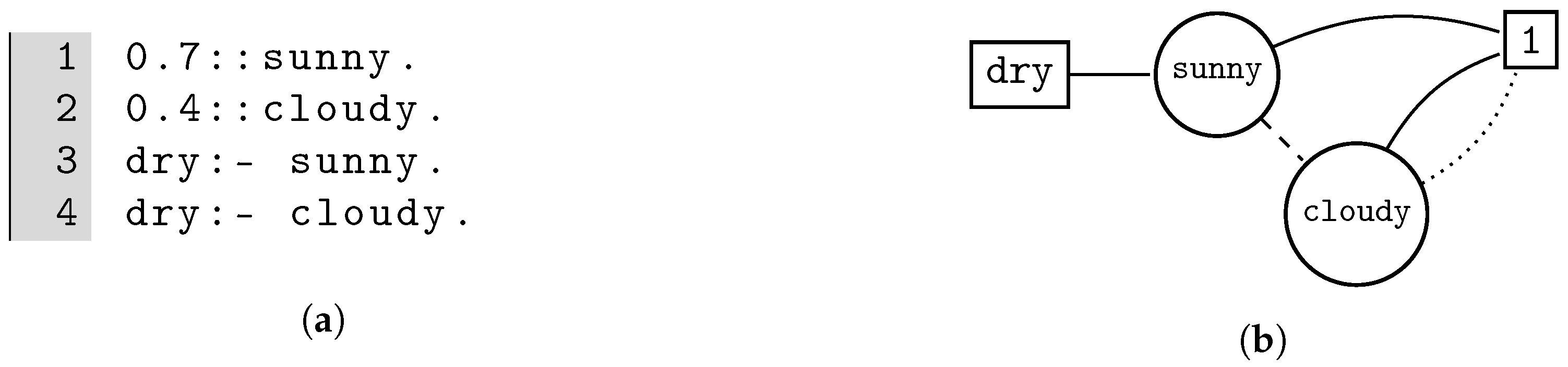
30]. For example, the program shown in
Figure 2a contains two probabilistic facts:
sunny, which is true with probability 0.7, and
cloudy, which is true with probability 0.4.
To compute the probability of a query in a probabilistic logic program (a task called
inference), we need to associate a precise meaning to a program, i.e., we need to choose a semantics for it. One of the most adopted semantics in the context of PLP is the Distribution Semantics (DS) [
32]. Following the DS, an
atomic choice indicates whether a grounding
for a probabilistic fact
f is selected. It is usually indicated with the triple
, where
. If
, the grounding is selected; otherwise, it is not. A consistent set of atomic choices (i.e., a set that does not contains both atomic choices
and
) identifies a composite choice
whose probability
can be computed with the formula
because we assume that probabilistic facts are independent. This assumption does not limit the expressive power [
4] of the language.
If a composite choice contains an atomic choice for every grounding of every probabilistic fact, it is called
total composite choice or
selection. A selection identifies a probabilistic logic program called
world, obtained by including in the program the facts that correspond to atomic choices with
. The probability of a world is the probability of the corresponding composite choice, and the sum of the probabilities of all the words of a program is equal to 1, so this way of assigning probabilities to worlds defines a probability distribution. Finally, the probability of a
query q,
, can be computed as the sum of the probability of the worlds
w where the query is true. In formula:
We consider queries composed by conjunctions of ground literals. The program in
Figure 2a has
worlds (two probabilistic facts): the first (
) where both
sunny and
cloudy are true, with an associated probability of
; the second (
) where
sunny is true and
cloudy is false, with an associated probability of
; the third (
) where
sunny is false and
cloudy is true, with an associated probability of
; the fourth (
) where both
sunny and
cloudy are false, with an associated probability of
. The query
dry is true in
,
, and
, and its probability is
. In general, the computation of the probability of a query is a #P-complete task [
33] since it involves counting all the possible solutions. To solve inference in practice, a probabilistic logic program can be converted into a different language, through
knowledge compilation [
34], in which the inference is easier. Here, we consider Binary Decision Diagrams (BDDs) as a target for the compilation.
A Binary Decision Diagram (BDD) is a rooted directed graph where each node has two outgoing edges, one associated with 1 (true, usually represented with a solid line), and one associated with 0 (false, usually represented with a dashed line). Terminal nodes can be either 0 or 1. Some BDD packages allow the definition of a third type of edge, the 0-complemented edge, usually represented with a dotted line, with the meaning that the function represented by the child must be complemented. With this third type of edge, the 0 terminal is not needed. The BDD associated with the program shown in
Figure 2a is shown in
Figure 2b. Starting from a BDD, it is possible to compute the probability of a query with a recursive algorithm [
29].
We can now extend the logic program of Example 1 to a probabilistic logic program by considering edges with an associated probability.
Example 2 (Probabilistic Path).
We can attach probabilities to the edge/2 facts of the program shown in Figure 1a. For example:The clauses for the predicatepath/2are unchanged. Now, all the edges have an associated probability, and thus the routing is probabilistic. Note that probabilistic and deterministic edges may coexist in the same program. We can compute the probability of the query path(a,e)using, for example, PITA [35], obtaining 0.3128. With systems like cplint [
36], it is possible to define
probabilistic clauses, i.e., clauses with an attached probability, with the syntax:
where, as before,
is an atom and
is a conjunction of literals.
is the probability associated with the clause. This can be encoded in ProbLog as:
where
f is an atom whose arguments are all the variables appearing in the rule.
Finally, with
flexible probabilities [
5], it is possible to define facts and clauses whose probabilities are not fixed but are computed during the program execution and may depend on input parameters. For example, in
the probability P of q/1 depends on the value of the argument A.
4.3. Probabilistic Abductive Logic Programming
Reasoning under incomplete data are a central task in abduction [
37]. In Abductive Logic Programming (ALP), atoms on which we have incomplete information are identified as
abducible. Moreover, an abductive logic program may also contain
integrity constraints (ICs) that limit the possible combination of abducibles. The goal is to find the minimal subset (here, we consider minimality in terms of set inclusion, but other alternatives are possible [
38]) of abducibles that explains a given query.
ALP inherits the main limitation of LP, namely, the impossibility to reason with uncertain data. Recently, the authors of [
39] introduced
Probabilistic Abductive Logic Programs (PALPs), where PLP is extended with the possibility to define
abducible facts with the syntax
where
a is an atom, and probabilistic integrity constraints with the syntax
where
is a conjunction of literals and
is the associated probability. The goal is to find the minimal set (in terms of set inclusion) of abducible facts
such that the joint probability of the query
q and ICs
is maximized. In formula,
where
The function is needed to remove the sets that yield the maximum joint probability but are not minimal.
Example 3 (Probabilistic abductive logic program). Consider the following probabilistic abductive logic program:
The first two lines introduce two abducible facts,aandb. The last line represents a deterministic integrity constraint () imposing thataandbcannot be both true at the same time. Given the queryq, the two sets = {a}and ={b}represent the solution of the abductive problem, both yielding a probability of 0.2 forq. Note that, if we remove the integrity constraint, the set Δ ={a,b}would have been the abductive explanation, with , but is forbidden by the IC.
4.4. Probabilistic Optimizable and Probabilistic Reducible Logic Programs
Two recently proposed extensions of PLP are Probabilistic Optimizable Logic Programs (POLP) [
40] and Probabilistic Reducible Logic Programs (PRLP) [
41]. Starting from the former, POLP extends PLP by adding
optimizable facts, with the syntax
where
and
are respectively the lower and the upper bound (
,
,
) for the probability for the fact
a. The values
and
may be omitted: in this case, they will be 0.001 and 0.999, respectively. The goal is to find the best probability assignments
to optimizable facts to optimize (minimize) an objective function
under constraints
, and then compute the probability of a query, in formula
and then compute
. If we consider the program introduced in
Figure 1 with all the edges defined as optimizable, a possible objective function could be the sum of the probabilities of all the edges, and a possible constraint could be keeping the probability of reaching
e starting from
a above a certain threshold.
Example 4 (Probabilistic Optimizable Logic Program). Consider the following Probabilistic Optimizable Logic Program:
The first two lines introduce two optimizable facts,aandb, each with a probability range between 0.3 and 0.9. If the goal is to minimize the sum of the probabilities of the two optimizable facts with the constraint that the probability ofqmust be greater than 0.3, a possible probability assignment for both facts is approximately 0.817, yielding a probability ofqof 0.3.
Similarly to POLP, PRLP extends PLP by adding
reducible facts with the syntax
where
a is a fact with associated probability
. The value
may be omitted. The goal is to find the subset with minimal cardinality
of reducible facts
such that the imposed constraints
are not violated. In the formula:
If we consider again the program discussed in Example 1 with all the edges defined as reducible, a possible constraint could be keeping the probability of reaching e starting from a above a certain threshold while removing as may edge facts as possible.
The difference between POLP and PRLP is that, in the former, the probability of the probabilistic fact can be set in the specified range, while, in the latter, the probability of the reducible facts is fixed, but reducible facts can be removed from the program (by setting their probability to 0).
Example 5 (Probabilistic Reducible Logic Program). Consider the following Probabilistic Reducible Logic Program:
The first two lines introduce two reducible facts,aandb, with an associated probability of 0.8 and 0.7, respectively. If the goal is to keep the probability ofqabove 0.15, the reducible factbcan be removed from the program: in this case, the probability ofqbecomes 0.16.
In the next section, we show how to adapt these models to describe and study the LN.
5. Lightning Network Models
The LN can be easily represented as a graph using the Prolog language [
16]. We focus here on a directed graph representation, but the discussed models can be easily extended to consider an undirected graph. Following [
15,
17], we consider a uniform distribution for the funds in a channel (i.e., its capacity)
c and define the
channel success probability (denoted as
) as the probability that a payment of size
S passes through a channel of capacity
C between two nodes. In formula,
if
and
, 0 otherwise. For example, for a payment of size
and a channel
c of capacity
, the success probability
is
. It is difficult to make further assumptions on the distribution since; as already discussed in previous sections, it is unknown. Moreover, a payment can be split across multiple channels. Given a path that connects two nodes, the
path success probability (PSP) [
15] is defined as the product of the channel success probabilities of the involved edges. We will use channel and edge interchangeably, both to identify a payment channel between two nodes.
Example 6 (Computing the path success probability with a Logic Programming model).
In [16], the authors represent each channel of the LN with a Prolog fact of the formWe can leverage this notation and easily adapt the model shown in Figure 1a to compute the path success probability, by adding an additional argument representing the capacity associated with theedge/2facts, as in [16]. To obtain the path success probability for a given path and a given payment size, the whole program of Figure 1a can be modified as follows: ![Cryptography 06 00029 i008]()
The network has the structure depicted in Figure 1b and, for simplicity, we set the total capacity for all the channels to 10. The arguments ofpath/6are the following: inpath(Source,Destination,PaymentSize,NodesInPath,InitialProbability,FinalProbability),Sourceis the source node,Destinationis the destination node, andPaymentSizeis the size of the payment that should be routed fromSourcetoDestination;NodesInPathis a list containing the nodes encountered in a path,InitialProbabilityis an accumulator for the probability (that starts from 1), andFinalProbabilityis the computed path success probability. In the first clause forpath/6(line 9), the source and destination nodes (Node) coincide, the list of nodes contains only one the current nodeNode, and the path success probability is the probabilityPaccumulated so far. Logic programming predicates are often recursive: in this example, the second clause for thepath/6predicate is the general case while the first is the base case (a path is found). Thepath/6predicate works as follows: first, it checks whether there is an edge between the current nodeSourceand an intermediate nodeIntermediate(line 11). The predicatechannelSuccessProbability/3checks whether the capacityCapacityof the selected channel is sufficient to route a payment of sizeSize(line 6) and then computes the channel success probabilityChProb. After this, the computed path probability is updated to account for the current value (line 13). Finally, the predicate is recursively called to find a path that connects the intermediate nodeIntermediateand the destination Dest.
If we consider a payment of size 2, there are two possible paths fromatoe, with an associated probability of each. We can retrieve these by asking the querypath(a,e,2,Path,1,Prob). We can likewise collect all the paths and associated probabilities in a list using the standard Prolog predicatefindall/3:
Moreover, by retrieving all the possible paths, it is easy to find the path that gives the maximum probability.
The computation of the PSP is straightforward since it considers only one path at the time, and the probability of a path is the product of the probabilities associated with all the involved edges. However, if we compute the probability to reach e starting from a, we get 0.69632 since both paths could route the payment.
In this paper, we focus on a different task than the computation of the PSP: the main goal is to provide models to reason about the probability of existence of a path that we call
path existence probability (PEP), between two nodes. As already discussed, edges in the LN can be considered as probabilistic, with an associated probability that depends on the size of the payment: if we consider a uniform distribution for the funds in a channel, payments with a small size (in terms of transferred funds) have higher probability to pass through an edge. To better see the difference between PSP and PEP, consider again the graph shown in
Figure 1b: if we fix the payment size such that every edge has an associated probability of 0.5, the PSP of both paths between
a and
e is
. However, the PEP between
a and
e is 0.21875 (given by, in compact form,
) and thus greater than the PSP of every individual path since both paths may route the same amount. This may be useful information in the context of Multi Path Payments, where payments are split and routed through multiple channels or in the case we try to route multiple times simultaneously the same amount. In these scenarios, the PEP represents the probability that
at least one of the payments succeeds. Overall, the PEP is an upper bound for the PSP: if there is only one path between two nodes, the PEP coincides with the PSP; otherwise, it is greater since it considers multiple paths together, and not only one. Finally, the computation of the PEP is more complex than the computation of the PSP since we cannot simply multiply the probability of the edges and sum the results. We now show a possible model to compute the PEP.
To account for the uncertainty distribution of the funds, we extend the previously discussed facts and predicates. First, we define a new probabilistic predicate connected/3 whose probability is defined using flexible probabilities. Its structure is:
where
P is the associated probability computed with the
channelSuccessProbability/3 predicate of Example 6. The definition of the
path/2 predicate shown in
Figure 1a is modified in:
If we consider again the network of
Figure 1a where, for simplicity, every edge has an associated capacity of 10, we can compute with PITA [
35] the probability of a path (PEP) between
a and
e that can route a payment of size 5 with the query
path(a,e,5), obtaining 0.21875. If we try to route instead a payment of size 7, with the query
path(a,e,7), we obtain 0.05157, a smaller value.
We further extend the model to consider intermittent nodes, representing a scenario where the routing of a payment through multiple edges may fail due to inactive nodes. To account for this, we can add a probabilistic fact
where p is a fixed number in . As before, we can adapt this fact to consider different probabilities for different nodes, by using flexible probabilities. The connected/3 predicate is further extended as
If we set the probability of active to 0.99, the probability of successful routing reduces: P(path(a,e,5)) = 0.21255 and P(path(a,e,7)) = 0.05006.
Finally, these predicates do not set a limit on the length of the path between two nodes. In multi-hop routing, every intermediate node between the source and the destination collects a fee. This implies that longer paths are more expensive than shorter paths. However, according to [
8], the average shortest path between two nodes is less than three steps. Here, we set the maximum length of a path to 5, to consider multiple non optimal (in terms of number intermediates nodes) paths. Longer paths have a lower associated success probability and thus provide a smaller contribution. Moreover, each additional step requires paying fees to intermediate nodes, so longer paths are also more expensive. We can easily set a limit on the length of the path by modifying the
path/3 predicate, as shown in Example 7.
Example 7 (Computation of the PEP between two nodes by considering only paths with a fixed maximum length). With the following program, it is possible to compute the probability of a path of length at most NMaxSteps that can route a payment of size Size between two nodes X and Y.
Thepath/5predicate counts the numberNStepsof encountered edges and compares it against the maximum numberNMaxStepsof allowed steps. For example, if we add the followingedge/3facts
we can compute the probability of routing a payment of size 5 betweenaandeby considering only the paths with length at most 3 withpath(a,e,5,3,0), obtaining 0.12128 (one of the two possible paths is discarded). However, if we set the maximum length to 4, the probability of the querypath(a,e,5,4,0)is 0.166465. For this example, if the maximum length is greater than 4, the probability does not increase.
5.1. Abductive Model
Abduction is a reasoning strategy applicable in scenarios with incomplete information. The proposal discussed in
Section 4.3 integrates abduction with uncertainty and makes it suitable to model the LN. For example, during the computation of the PEP, a user can impose that some edges must not be considered together. Moreover, there can be edges not publicly advertised. These two situations can be modelled with abducible facts and integrity constraints.
Let us consider the model shown in Example 7, with active probability set to 1. We can denote some edges as abducibles and insert an integrity constraint, in this way:
![Cryptography 06 00029 i016]()
The network is the one depicted in
Figure 1b. The (deterministic) integrity constraint states that the edges between
a and
b and
c and
e cannot be selected at the same time. With this program, the set of abducibles that maximizes the joint probability of the query
path(a,e,2,5,0) and the constraint is
{edge(a,b,10)}, which yields a probability of 0.2133. If we associate a probability of, for example, 0.3, to the constraint, indicating that we are unsure about the information it provides, we get the set
{edge(a,b,10),edge(c,e,10)}, yielding a probability of 0.3957. From a user perspective, identifying the most important edges can be of interest since he/she may decide whether to insert more connections to provide possible alternatives in case of attacks or nodes that decide to not forward a payment. From an attacker perspective, he/she can identify the most important edges for a given target node and try to block them, for example, with “lockdown attacks” [
12].
Note that, with this model, we can insert the constraint :- e(A,B), e(A,C), B \= C, imposing that there must not be two edges that share the same source node and set all the edges as abducible to compute the PSP. However, this constraint is computationally very expensive since it requires the generation of all the possible triples of nodes.
5.2. Optimizable Model
In our models, the funds locked in an edge directly characterize its probability, once the payment is fixed. Thus, with POLP, we can impose some constraints and consequently set the probabilities (and thus the funds) of the channels to target an objective function.
We start from the model shown in Example 7, but we set some of the edge/3 facts related to nodes as optimizable. Consider the following edges:
![Cryptography 06 00029 i017]()
The last two are optimizable and their probability can be set. The probability of the active/1 facts is set to 1. Suppose that the goal is to optimize the probability of the query path(a,e,2,5,0). The objective function requires minimizing the sum of the probabilities of edge(b,d,3) and edge(d,e,10) (i.e., the objective function is P(edge(b,d,3)) + P(edge(d,e,10))). At the same time, the probabilities of the two optimizable facts must be close (for example, with a difference less than 0.1). Furthermore, the probability of the query path(a,e,2,5,0) should be above or equal to 0.5. With all the edge/3 facts deterministic, the probability of the query is 0.565. The solution of the optimizable problem consists of assigning probability 0.4841 to both optimizable facts. As discussed before, the channel success probability is given by , where C is the capacity of the channel and S is the size of the payment. By considering some of the edge/3 facts as optimizable, we assign to them a second probability value, call it , that will be computed with the model. We can use this new value to find the optimal capacity of a channel by solving the following equation in terms of : . In this way, we get . For this example, the new funds will be for the edge between b and d and for the edge between d and e, obtaining a probability of 0.5 for the query.
With this model, it is possible to compute the optimal amount of funds to associate to edges. Moreover, if we consider instead the active/1 facts as optimizable, we can compute the optimal probability to accept or reject a payment while guaranteeing, at the same time, some probability bounds for certain paths. From the perspective of a node, this may be useful to prevent, for example, a possible subsequent imbalance in the distribution of funds in the involved channels. An imbalance in a channel requires the adoption of some mechanisms such as “rebalancing” to restore its funds to one of the two ends. Moreover, if a channel is unbalanced, a node may not be able to route payments through it, possibly reducing its earnings, and this can be a possible target for an attacker.
5.3. Reducible Model
With PRLPs, as discussed in
Section 4.4, some facts are considered “reducible” and removed from the program. The goal is to minimize the number of reducible facts kept in the program while ensuring the validity of some constraints. These types of programs can be used, for example, to spot the nodes and edges that provide a substantial contribution in the routing, or, on the other hand, nodes that can be ignored. For example, if we want to perform some analyses on certain nodes, we can first apply this model to identify the essential edges and then focus on the remaining ones, greatly simplifying and reducing the size of the considered graph. Moreover, this model can be applied as a pre-processing step for the routing of a payment or for locating the best position for a possible new connection. In this last case, we can add some edges to the LN model, with different capacities and that connect different source destination couples. Then, we can set a target probability of a successful routing, remove the not needed edges, and create only the identified ones on the real LN.
To illustrate this, we keep the model shown in Example 7 but we consider all the edges as reducibles. For example, consider the program
representing
Figure 1b. We may impose that the probability of reaching
e from
a must be greater than 0.4. With all the facts included, and the probability of the
active/1 facts set to 1, the probability of the query
path(a,e,2,5,0) is 0.5653. However, by removing
edge(b,d,3), we obtain a probability for the same query of 0.48, satisfying the constraint. Thus, the identified edge can be removed. From an attacker perspective, this can be interesting since he/she can identify the edges that a target user must preserve to route a payment of a given size, and consequently try to attack them, to disclose, for example, the balance distribution in the edges.
6. Experiments
We perform multiple experiments on a computer with Intel® Xeon® E5-2630v3 running at 2.40 GHz to illustrate some possible statistics obtainable with our models.
Following previous results [
8,
10], the Lightning Network can be considered as a
small-world and
scale-free network [
42] network since there are a few nodes with a high degree and many nodes with a low degree. Thus, for every experiment, we generated 50 random network structures (i.e., random
edge/3 facts) using the method
scale_free_graph from the “networkx” Python package [
43,
44] and averaged the results. We used the default parameters for the generation of the networks:
, the probability for adding a new node connected to a randomly existing node according to the in degree distribution, set to 0.41,
, the probability for adding an edge between two existing nodes, set to 0.54, and
the probability for adding a new node connected to an existing randomly chosen node according to the out-degree distribution, set to 0.05. The biases for choosing nodes from in-degree and out-degree distribution are, respectively, set to 0.2 and 0. We discarded the edges with the same source and destination. The average number of edges for every experiment is shown in
Table 1 and
Table 2.
We can likewise test our approach on the real Lightning Network, by taking a snapshot of it. However, the LN is in continuous change: results computed on a snapshot can be obsolete in a few weeks, even days. Moreover, since we select random source and destination nodes with distance at most 5, we will likely get a lot of disconnected pairs. The selected source–destination pair changes for every instance and every payment size. Finally, our models do not aim to perform (even if they can) an analysis of the whole LN; rather, the goal is to see how the discussed models can be applied to provide some indications regarding small subsets, since users are usually interested in contacting a small group of nodes, and it is unlikely that they will interact with all the nodes in the network.
We consider a directed graph where nodes are indexed with whole numbers and, for each fact of the form
edge (A,B,Capacity),
B >
A, to ensure acyclicity. To associate capacities to edges, we selected random capacities from a snapshot of the LN from the 12 April 2021 [
17] composed of 14,734 nodes and 44,349 channels. In this snapshot, approximately 80% of edges have less than the average capacity (2,837,035 satoshi), 72% have less than half of the average capacity, and 59% have less than a quarter of the average capacity. We tested the routing of payments of sizes 4651, 11,629, 22,258, 46,516, and 116,296 satoshi, which correspond, at the moment of writing, to approximately 2, 5, 10, 20, and 50 dollars, between 10 random pairs of nodes for every experiment. The paths go from
A to
B, with
B >
A to account for the order imposed in the generation of the edges. Note that, as in the real LN, there can be nodes connected by multiple edges.
For all the experiments, first we selected two random connected nodes that can route a payment of a certain size, i.e., connected by a path where all the edges have total capacity greater than the payment size. Then, we apply the considered model. In this way, we avoid reasoning on nodes that, even if connected, cannot route the desired amount. We do this because, if there is not a path between two nodes, clearly the probability is 0, so there is no reason to attempt a payment.
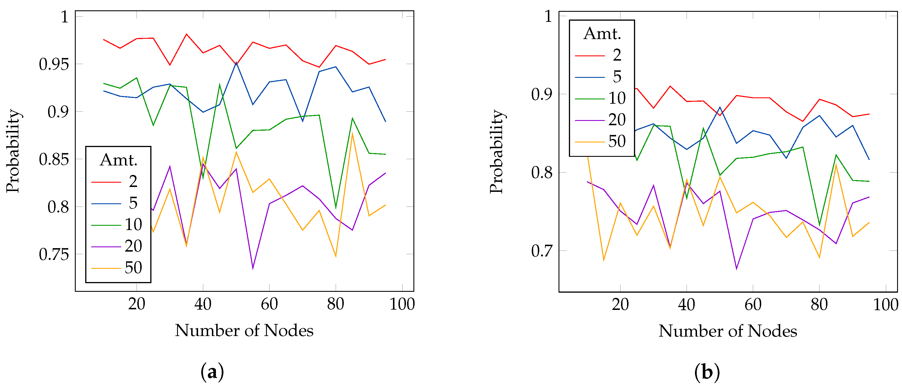
For the path existence probability experiments, we generated random network structures with a size (number of nodes) from 10 up to 100 with step 10. We plot how the PEP varies by increasing the number of nodes (and thus edges) in the networks and by increasing the payment size. We consider the same networks first with all the nodes always active (active probability set to 1) and then with an active probability of 0.95. From the results shown in
Figure 3, the PEP increasingly varies when the number of existing nodes and the size of the payments increases. This may happen because channels with a total capacity close to the payment size have a small probability to route the payment. The results on networks where each node has an active probability of 0.95 present a similar behaviour to the ones obtained with nodes always active, with a difference of at most 10% in the path existence probability.
For the abductive and optimizable models, we generated random network structures with a size (number of nodes) from 5 up to 20 with step 1. For reducible models, the network size varies between 5 and 10.
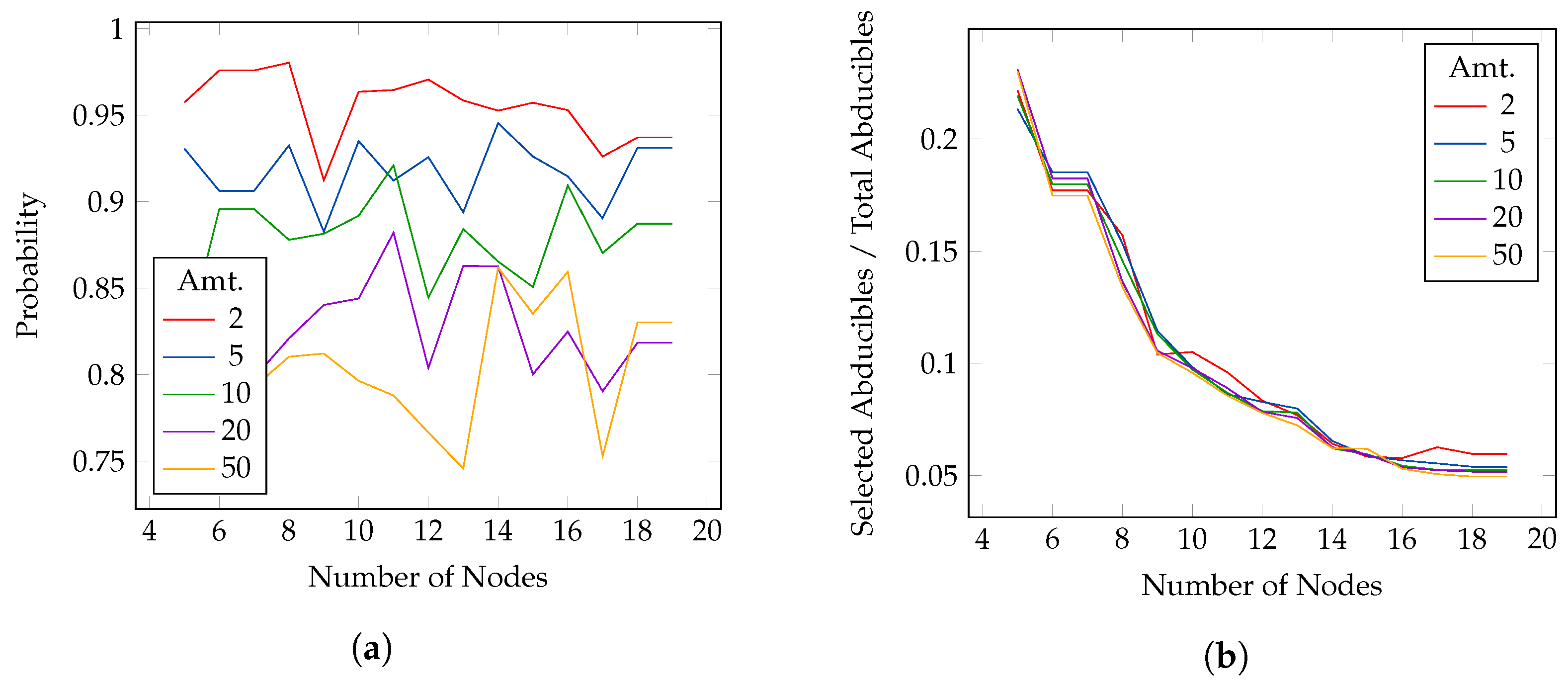
For the abductive model experiments, we randomly set half of the total edges of the networks as abducibles and insert a number of constraints equal to one quarter of the total number of edges. These constraints are deterministic and encode the incompatibility of a random pair of abducible edges each. The plots of
Figure 4a,b show respectively the variation of the PEP and of the ratio between the selected abducibles and the total abducibles involved in the computation, with an increasing number of nodes (and thus of edges) and an increasing payment size. The active probability is set to 1. The variation of the PEP, as for the previous experiments, increases by increasing the payment size. However, the number of selected abducibles to maximize the PEP decreases as the number of nodes and edges increase, meaning that few nodes are involved in the routing process. This variation is similar for all the five amounts tested. For both this and the previous experiment, there are several jumps in the computed probability values. These jumps are more evident for bigger amounts, thus indicating that the choice of the payment size and the existing connection is crucial.
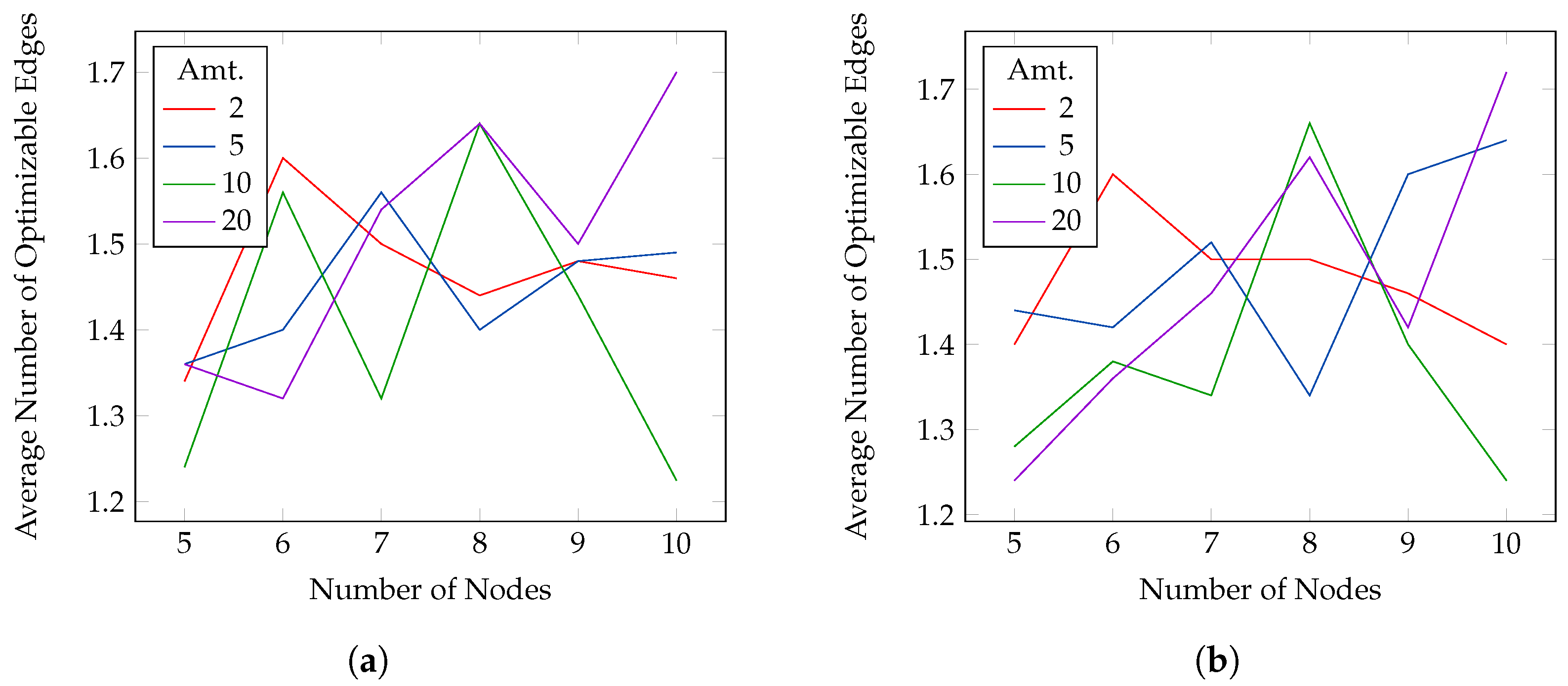
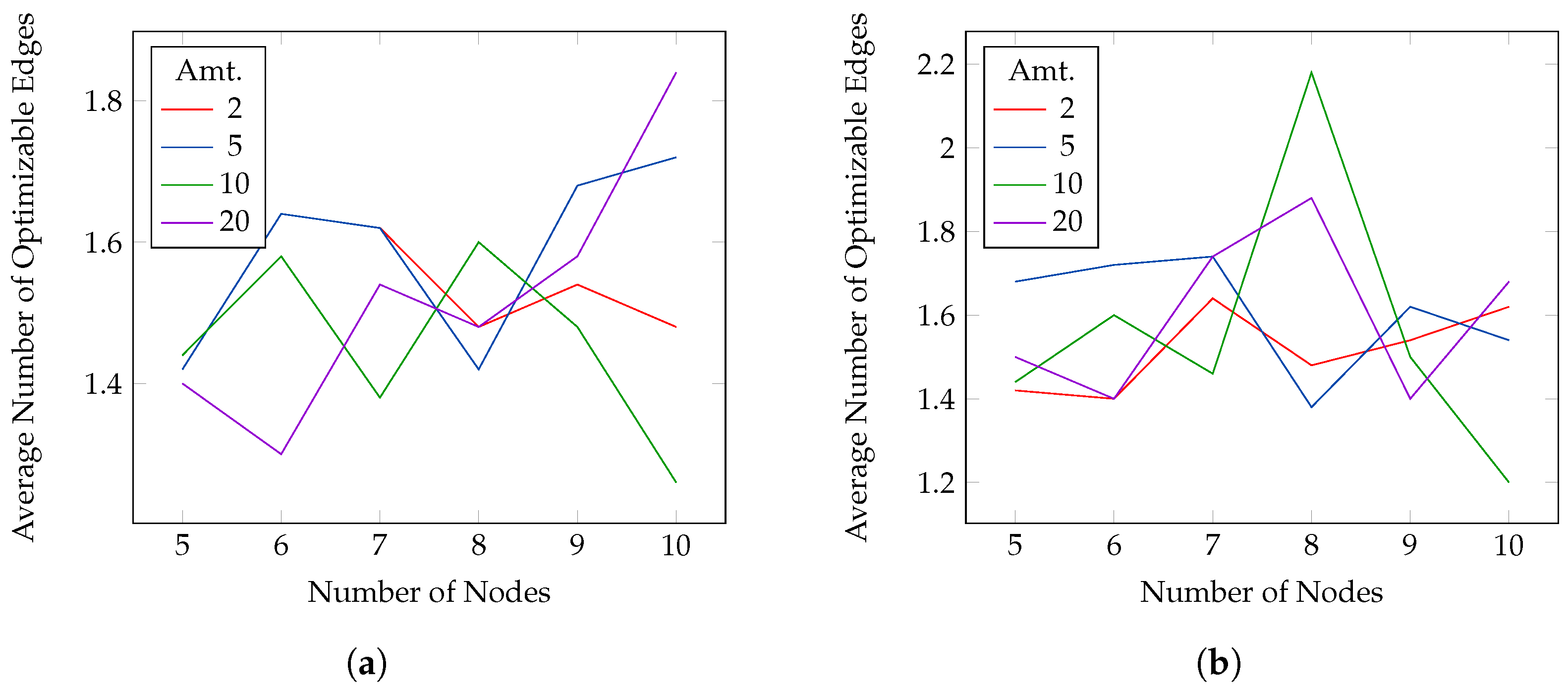
For the optimizable experiments, we consider all edges as optimizable, with probability ranges between 0.001 and 0.999. The goal is to minimize the sum of the probabilities of the edges while, at the same time, keeping the probability of path between two random pairs above 0.6, 0.7 (
Figure 5) 0.8, 0.9 (
Figure 6). The source–destination pair is the same for the four thresholds but changes for every instance and payment size. The figures show, on the
y-axis, the average number of edges involved in the optimization (i.e., with probability different from the lower bound 0.001), and on the
x-axis the number of nodes. In each figure, there are five plots, representing different payment size. For all, the active probability is set to 1. Results are similar for all the payment sizes and indicate that usually the average number of involved edges is between 1.4 and 1.6 and, at most, two edges are needed to reach the desired probability. When the probability threshold increases, the number of edges slightly increases but not drastically.
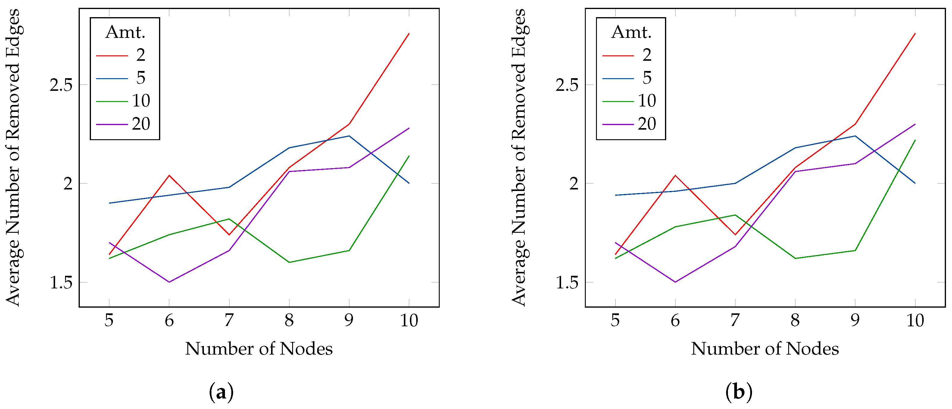
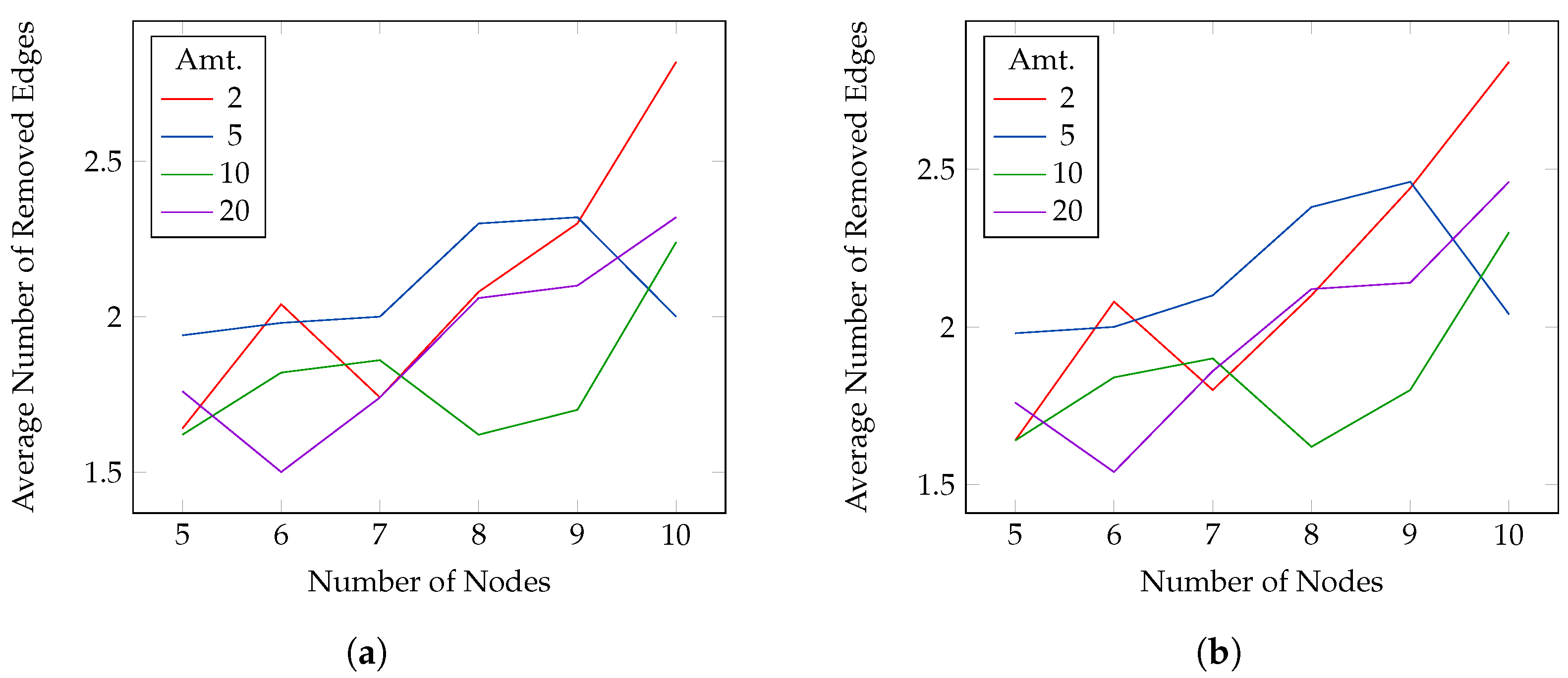
For the reducible experiments, we set all edges as reducible. The goal is to remove as many edges as possible while keeping the PEP between two random nodes above 0.6, 0.7 (
Figure 7) 0.8, 0.9 (
Figure 8). As for the optimizable experiment, the source–destination pair is the same for the four thresholds but changes for every instance and payment size. We chose the approximate algorithm. The figures show, on the
y-axis, the average number of removed edges and on the
x-axis the number of nodes in the network. For all, the active probability is set to 1. In this case, the number of selected edges is small with respect to the number of nodes, and it is usually bounded between 1.5 and 3. The results are similar for all the thresholds, but, in general, smaller payments allow for removing more edges.


