Article

Evaluation of Contributing Factors Affecting Number of Vehicles Involved in Crashes Using Machine Learning Techniques in Rural Roads of Cosenza, Italy

by
Giuseppe Guido
1,
Sina Shaffiee Haghshenas
1,
Sami Shaffiee Haghshenas
1,
Alessandro Vitale
1,
Vittorio Astarita
1,*,
Yongjin Park
2,* and
Zong Woo Geem
3
1
Department of Civil Engineering, University of Calabria, Via Bucci, 87036 Rende, Italy
2
Department of Transportation Engineering, Keimyung University, Daegu 42601, Korea
3
College of IT Convergence, Gachon University, Seongnam 13120, Korea
*
Authors to whom correspondence should be addressed.
Safety 2022, 8(2), 28; https://doi.org/10.3390/safety8020028
Submission received: 17 December 2021 / Revised: 27 March 2022 / Accepted: 30 March 2022 / Published: 8 April 2022

Abstract

:
The evaluation of road safety is a critical issue having to be conducted for successful safety management in road transport systems, whereas safety management is considered in road transportation systems as a challenging task according to the dynamic of this issue and the presence of a large number of effective parameters on road safety. Therefore, the evaluation and analysis of important contributing factors affecting the number of vehicles involved in crashes play a key role in increasing the efficiency of road safety. For this purpose, in this research work, two machine learning algorithms, including the group method of data handling (GMDH)-type neural network and a combination of support vector machine (SVM) and the grasshopper optimization algorithm (GOA), are employed. Hence, the number of vehicles involved in an accident is considered to be the output, and the seven factors affecting transport safety, including Daylight (DL), Weekday (W), Type of accident (TA), Location (L), Speed limit (SL), Average speed (AS), and Annual average daily traffic (AADT) of rural roads in Cosenza, southern Italy, are selected as the inputs. In this study, 564 data sets from rural areas were investigated, and the relevant, effective parameters were measured. In the next stage, several models were developed to investigate the parameters affecting the safety management of road transportation in rural areas. The results obtained demonstrated that the “Type of accident” has the highest level and “Location” has the lowest importance in the investigated rural area. Finally, although the results of both algorithms were the same, the GOA-SVM model showed a better degree of accuracy and robustness than the GMDH model.

1. Introduction

Road transport is one of the oldest methods of transporting goods and individuals. With the increase in the population and the development of towns, the expansion of road transport has become an inevitable issue that plays a significant role in increasing and improving economic and social development. Numerous issues affect the quality and quantity of road transport, and safety management is one of the most significant subjects. Therefore, identifying, studying, and evaluating the contributing factors affecting road safety is inevitable to increase the level of safety management. Several parameters affect road safety, and valuable studies have been conducted to investigate road safety, such as Driver Behavior [1,2,3,4,5,6,7], Age of Driver and Vehicle [8,9,10,11,12,13], Weather Conditions [14,15,16,17,18], Road Geometry [19,20,21,22,23], and Lighting Conditions [24,25,26,27,28,29]. Siliquini et al. (2010) investigated the link between driving performance and the use of psychoactive drugs in teen drivers who were enrolled at common consuming locations. For this purpose, they designed and implemented the TEND by Night project in several European countries. Based on their results, the key findings were the change in response time between entering and exiting the recreation site, as well as its relationship with psychoactive drug usage [30]. Alonso et al. (2017) studied a relatively large statistical community of drivers to explore the behavioral and representational characteristics of drivers that modulate the smoking–accidents relationship. They discovered that, despite being aware of the consequences of smoking while driving, few drivers thought it was a risky behavior. Finally, they suggested various recommendations based on their findings, such as increasing awareness and control of this habit [31]. Zoe et al. (2018) carried out an efficient analysis of the expansion trend in road safety research between 2000 and 2018. Their results indicated that road safety research focused on five major areas, including accident frequency data investigation, driver behavior questionnaire, safety in numbers for walkers and bicyclists, injury and prevention of road traffic, and driving speed and road accidents [32].
Moreover, other comprehensive studies have been performed to examine the role of other factors on road safety. Gichaga (2017) reviewed the historical and cultural backgrounds involving road development and road safety features in Kenya. Based on his results, he made some recommendations for improvements in aspects of road safety [33]. Elvik et al. (2019) conducted a review of the relationship between speed and road safety. They supported two mathematical models. Their results showed that the speed of individual drivers has a similar relationship with safety as the mean speed of traffic [34]. In another study, the effect of air quality on road safety was evaluated by Sager (2019). He investigated the impact of increased air pollution on the amount of road traffic crashes. Then, he found out that there is a relationship between the number of accidents and the amount of PM2.5 [35].
On the other hand, several techniques exist to evaluate the parameters affecting road safety. Traditionally, classical before–after research works, statistical modeling, and personal judgment-based approaches are applied to chronological data [36]. Zheng et al. (2018) investigated the proposal of a bivariate extreme value model. Their proposed model could reduce the uncertainty in crash estimates [37]. Moreover, according to a bivariate extreme value theory (EVT) framework, Wang et al. (2019) introduced an accident forecast method. Their results prove that the proposed crash prediction method can provide very promising results compared to univariate models [38]. In another research work, Zheng et al. (2020) carried out a comprehensive review of research based on traffic conflicts in the road safety analysis. Then, they discussed conceptual and methodological matters related to traffic conflict modeling. Based on their results, it has been determined that although suitable research studies have been performed on this issue, the need for more studies is necessary [39]. An overview of road traffic accidents was conducted in the Eastern Province, KSA, from 2009 to 2016 by Jamal et al. (2020). They developed logistic regression models to forecast crash severity. Finally, they recommended some suggestions to prevent road accidents [40].
Due to the uncertainty and unforeseen conditions of parameters affecting road safety and the high ability of machine learning algorithms to solve complex problems, recently, the use of these methods in combination with classical methods or, in many studies, alone has been widely used [41,42,43,44,45,46,47,48,49]. Xu et al. (2018) evaluated the effect of road lighting on road safety using an artificial neural network. The results clearly showed that road lighting greatly contributed to road safety levels [50]. In another study, two types of artificial intelligence methods were applied to estimate the severity of crashes by Amiri et al. (2020). They used the crash information from California in 2012. Their results indicated that both artificial intelligence models were reliable for predicting the severity of crashes, and also, the light condition played an essential role in the severity level compared to the other contributing factors [51]. Guido et al. (2020) investigated some potential factors for road safety using two artificial intelligence methods. Their results indicated that the PSO algorithm had a superior function compared to the GA algorithm for evaluating factors in road accidents [52]. Shiran et al. (2021) carried out crash severity analysis by applying data mining approaches and multinomial logistic regression. They used an accident dataset of State Highways in California, USA. They found that the C5.0 model provides a higher performance capacity in evaluating crash severity analysis than other models [53]. A brief review of the literature is shown in Table 1.
Studies of the past literature show that although valuable studies have been done, more research is needed to improve the quality of road transport based on the increasing expansion. Therefore, in this study, two machine learning algorithms, including the group method of data handling (GMDH)-type neural network and a combination of support vector machine (SVM) and the grasshopper optimization algorithm (GOA), are applied. Then, the obtained results of two algorithms are compared based on performance indicators to determine the performance of the models regarding the conditions and characteristics of a case study. Finally, a sensitivity analysis was conducted to prioritize the contributing factors affecting the number of vehicles involved in crashes in rural areas.

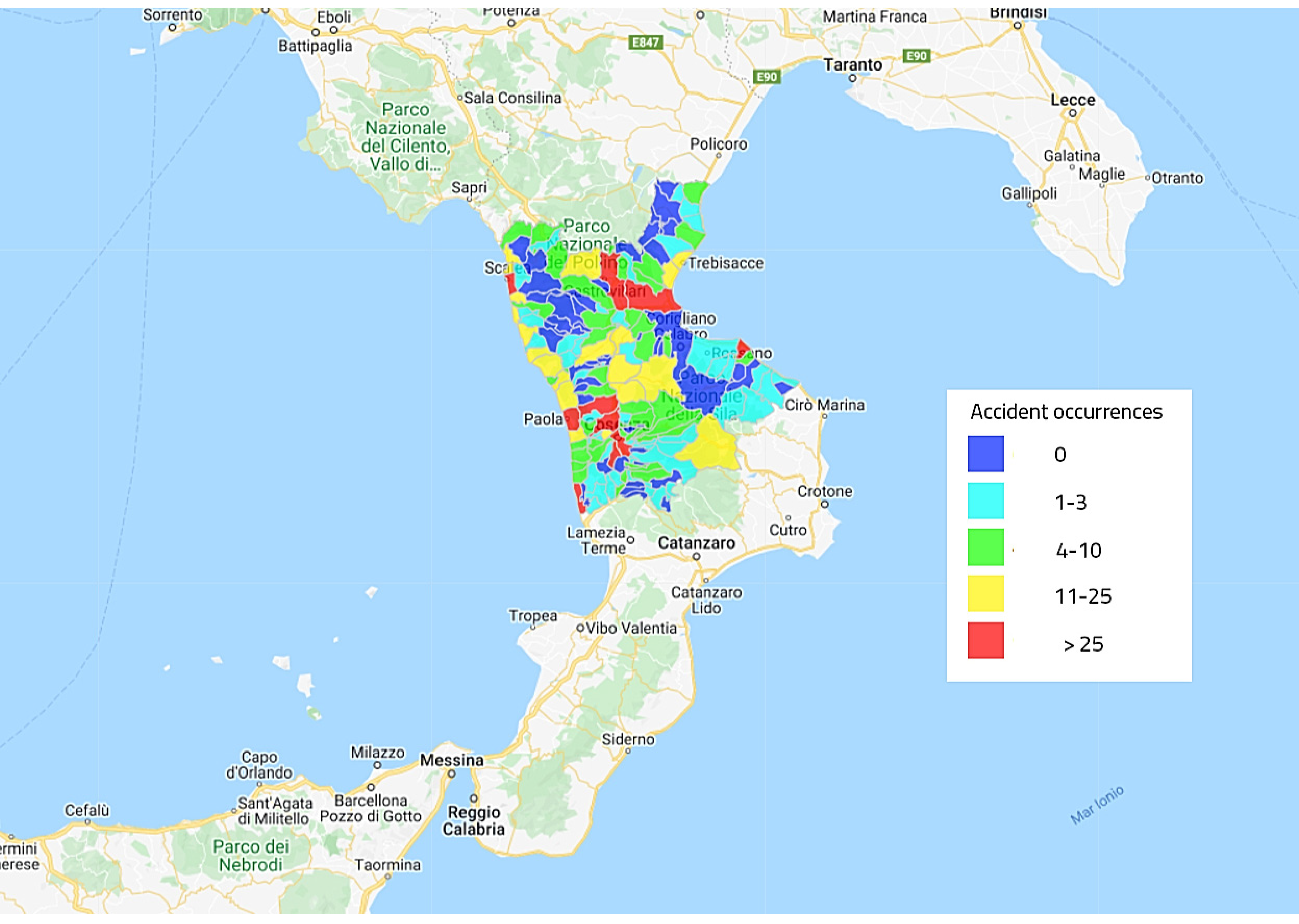
2. Site Description and Accident Monitoring

To evaluate the performance and usefulness of the proposed approaches for prioritizing the contributing factors affecting the number of vehicles involved in crashes in a rural area, a sample of 564 accident data was acquired from 2017 to 2018 on the rural road network of Cosenza province and has been analyzed (Figure 1). It should be noted that the most comprehensive data sets were available for modeling in this period.
The accident data has been acquired from the Automobile Club Italia (ACI) database, which collaborates with the National Institute of Statistics (ISTAT) in collecting road accident data in Italy. This database provides a lot of information about accidents, such as date and place, road category, pavement conditions, weather conditions, crash dynamics, the type of vehicle involved, the causes of the accident, and the consequences for the people involved (injuries or deaths). The information does not include Property Damage Only (PDO) events under existing Italian legislation, defining road accidents as accidents only when they cause at least one injury [54].
According to ISTAT, accidents are classified as fatal or with injuries; therefore, it is not possible to distinguish the injured according to the level of severity. Based on the previous comment, in this paper, the measure of the number of vehicles involved in an accident, as referred to in Section 4, is expressed as a dichotomous variable (0,1):
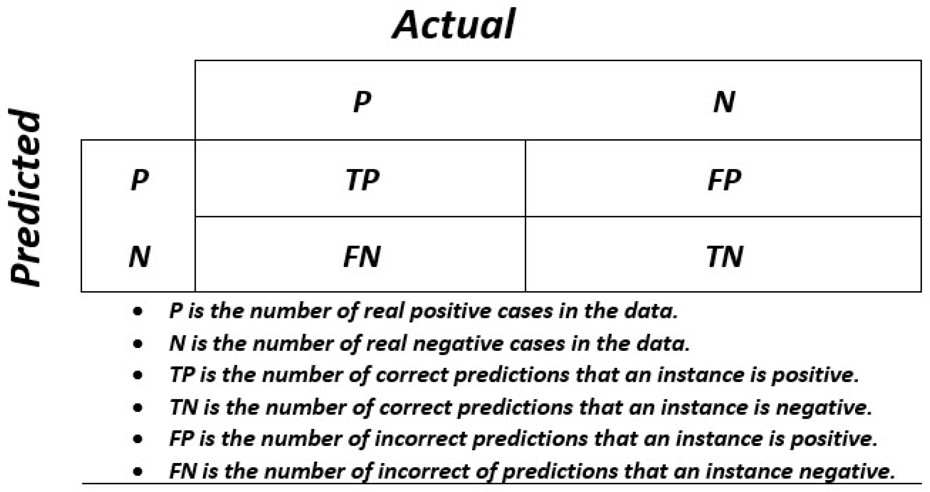
  • - When there is a vehicle involved in an accident, label 0 is considered.
  • - When there is more than one vehicle involved in an accident, label 1 is considered.
Other information on roads and traffic flows was considered to ensure a more detailed analysis, such as speed limits, average speed, and average annual daily traffic (AADT). The speed limits are regulated by the “Nuovo Codice della Strada” [55,56], and their values have been acquired from the database of Azienda Nazionale Autonoma delle Strade (ANAS). The average speed was obtained through the available data of the historical traffic statistics of TomTom (TomTom Move) and Octo Telematics (Octo IoT Cloud), referring to the road sections with the observed accidents. The AADT was acquired from the PANAMA system of ANAS (ANAS Platform for Monitoring and Analyzing).
This study considers seven independent variables (i.e., the factors affecting the number and severity of accidents), which were selected based on all the available data for the case study. These variables include four qualitative variables (Daylight (DL), Weekday (W), Type of accident (TA), and Location (L)) and three quantitative variables (Speed limit (SL), Average speed (AS), and Annual Average Daily Traffic (AADT)).
Table 2 shows the variables mentioned above, which are classified into various categories (codes) with their statements. The method of grouping variables into different categories depends on their characteristics and the number of observations involved in each study.

3. Methodology

The study of road safety is one of the inseparable issues of transportation engineering, which is usually defined by the absence of accidents and casualties. Lack of attention to road safety could impose irreparable financial and physical damages. Therefore, it is necessary to have a deep understanding of road safety, know all the effective components, and estimate the impact of each on this issue. Studying the literature reveals that most investigations in the field of road safety are based on logit models or regression models with artificial neural networks. On the one hand, the complexity and uncertainty of the factors affecting road safety, and on the other hand, the ability of machine learning algorithms to predict and navigate in the face of unexpected and uncertain issues, has resulted in the successful application of machine learning methods in road safety in recent years [57,58,59,60,61,62,63].
Accordingly, the main aim of this study is to investigate the factors affecting road safety in rural areas by using two machine training approaches, namely the GMDH model and the hybrid GOA-SVM model. For this purpose, the GMDH model was developed to achieve the best binary classification model by determining the best control parameters for GMDH. Moreover, the SVM was hybridized with the grasshopper optimization algorithm as a suitable evolutionary algorithm and was developed to optimize its three parameters. Finally, a sensitivity analysis was performed to evaluate and rank factors affecting the number of vehicles involved in an accident in rural areas. More discussions regarding machine learning models will be given in the next sections.

3.1. Group Method of Data Handling-Type Neural Network

In today’s science, ANNs (as one of the branches of artificial intelligence) play a valuable role in the development of new technologies. Therefore, the use of ANNs to solve many complex problems in various fields of science is inevitable [64,65,66,67,68,69,70,71]. The group method of data handling (GMDH) is one of the artificial neural networks that was introduced by Ivakhnenko (1971). The GMDH has been successfully used for computer-based mathematical modeling in complex systems, as well as data mining, optimization, and pattern recognition problems [72]. The process of GMDH is similar to a type of self-organizing network [73,74]. The mapping between the input and output variables in a GMDH neural network is a nonlinear function. The Polynomial Neural Network (PNN) is one of the basic algorithms used to construct GMDH models. In GMDH modeling, input data are entered into the initial layer, and, after preparation, they are considered input for the second layer, and this process continues until the algorithm converges and stops. Finally, in the convergence process of the algorithm, if the results in the layer (n + 1) are better than the layer (n), then the algorithm converges. Equations (1) and (2) indicate the relationship between the approximate function ( f ) with the multi-input and single-output ( y ) dataset and the least possible error between actual and predicted values [73,74].
y = f ( x i 1 , x i 2 , x i 3 , x i m ) i = ( 1 , 2 , 3 , , n )
i = 1 M [ f ( x i 1 , x i 2 , x i 3 , x i m ) y i ] 2 M i n
Equation (3) indicates a relationship between a single output (y) and a multi-input (Input vector, X = (x1, x2, x3, …, xm)) according to the Kolmogorov–Gabor polynomial [75,76].
y = a 0 + i = 1 m a i x i + i = 1 m j = 1 m a i j x i x j + i = 1 m j = 1 m k = 1 m a i j k x i x j x k + i = 1 m j = 1 m k = 1 m l = 1 m a i j k l x i x j x k x l ,
where a i , a i j , a i j k , a i j k l , are considered to be coefficients of the polynomial, and m is the amount of data. Furthermore, Equation (3) can be considered as a quadratic polynomial for 2 inputs according to Equation (4) [77].
y ^ = G ( x i , x j ) = a 0 + a 1 x i + a 2 x j + a 3 x i 2 + a 4 x j 2 + a 5 x i x j
The total error (E) is considered by minimizing the difference between the actual output (y) and predicted output ( y ^ = G ( x i , x j ) ) for each pair of input variables x i and x j based on Equation (5). Moreover, the coefficients of each quadratic function are optimized [78].
E = i = 1 M ( y i G i ( x i , x j ) ) 2 M M i n
Out of a total of n input variables, all alternatives for two independent variables are provided in the elementary form of the GMDH algorithm for providing the regression polynomial in the form of Equation (4) [79]. Therefore, ( n 2 ) = n ( n 1 ) 2 neurons will be made in the primary layer of the feedforward neural network from the observations { ( y i , x i , x i q ) ; ( i = 1 , 2 , 3 , , M ) } for various ( p , q { 1 , 2 , 3 , , n } ) . The matrix form of Equation (4) can be considered to indicate the main form of the GMDH based on Equation (6) [80].
Y = A a
Y = ( y 1 , y 2 , y 3 , , y m ) and a = ( a 1 , a 2 , a 3 , a 4 , a 5 ) are considered the observed output vector and the vector coefficient of the quadratic polynomial, respectively. A is computed based on Equation (7) [81,82].
A = [ 1 x 1 p x 1 q x 1 p x 1 q x 1 p 2 x 1 q 2 1 x 1 p x 1 q x 1 p x 1 q x 1 p 2 x 1 q 2 . . . . . . . . . . . . . . . . . . 1 x M p x M q x M p x M q x M p 2 x M q 2 ]
Finally, using the least-squares process from multiple regression analysis, a normal equation is achieved based on Equation (8), which calculates the vector of the best coefficients for Equation (4) [83].
a = ( A T A ) 1 A T Y

3.2. Support Vector Machine

A support vector machine (SVM) is an effective machine learning method that was introduced by Cortes and Vapnik (1995) [84]. SVMs are a kind of supervised learning algorithms that are used in a wide range of modelings, such as regression and classification. The SVM presents a linear two-class classifier and aims to maximize the margin amongst two classes so that a classification hyperplane is formed in the center of the maximum margin. It provides many hyperplanes, while the goal of the support vector machine is to find the best hyperplane in n-dimensional space. Two labels are considered for this classification: label +1 is considered for cases that are above the hyperplane, and label −1 belongs to cases that are under the hyperplane. Equation (9) shows a group of the sample set that is used in classification learning data [85,86].
S = { ( x i , y i ) i = 1 n | x i R N , y i { 1 , 1 } , i = 1 , 2 , , l }
where y i is the target variable for the observed i-th sample (the sample category). It is also assumed that x i presents the i-th sample data. After the formation of hyperplanes, one of the hyperplanes has the highest margin, which is called the optimal hyperplane. This optimal hyperplane is determined by the existing support vectors and constraints. Equations (10) and (11) indicate the constraints [87,88].
M i n 1 2 w 2
s . t . y i ( w x i + b ) 1
where w and b are the weight vector and the bias vector, correspondingly. Then, considering an error coefficient, the constraints are rewritten and corrected according to Equations (12) and (13). This error coefficient is intended to ensure a more accurate classification [88].
M i n 1 2 w 2 + c i = 1 n ε i ( ε i 0 )
s . t . { y i ( w x i + b ) 1 ε i c 0 ( i = 1 , 2 , 3 , , n )
where c is the penalty coefficient. Then, using the Lagrange method, SVM classification problems are considered as the following dual optimization problem based on Equation (14) [88].
{ W ( a ) = i = 1 n a i 1 2 i , j = 1 n a i a j y i y j K ( x i , x j ) s . t . i = 1 n a i y i ( 0 a i c ; i = 1 , 2 , 3 , , n )
where K is a mathematical function that is called the kernel function. There are different types of kernel functions, including linear (LIN), the radial basis function (RBF), and polynomial (POL), and their relationships are shown in Table 3. Gamma ( γ ) and d are necessary to define the kernel types. Gamma ( γ ) is used for RBF and POL and “d” represents the term of polynomial degree only for the POL kernel function [89,90]. The most important role of the kernel function is to take the dataset as an input and convert it into the required form. Knowledge of the use of various kernel functions in related situations can affect the quality of the category.

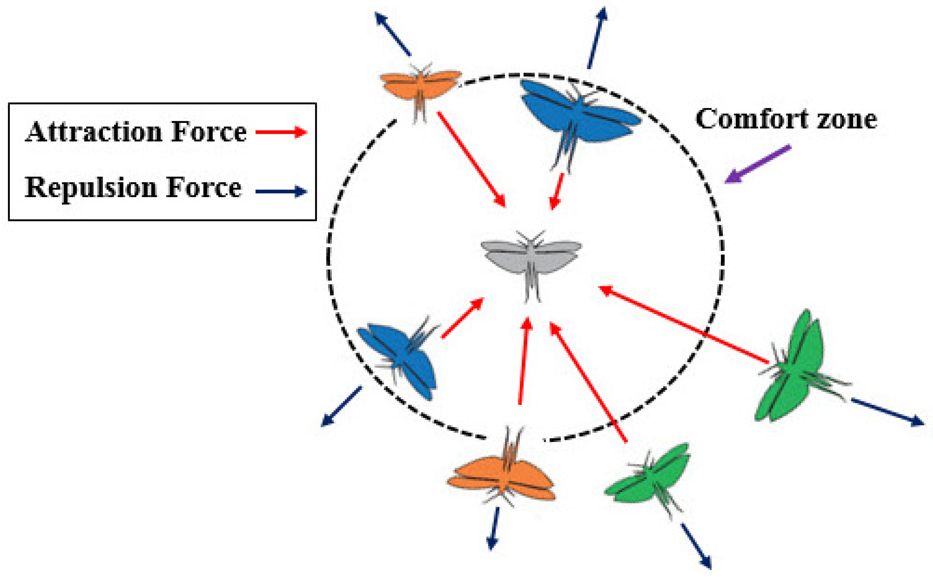
3.3. Grasshopper Optimization Algorithm

In recent years, meta-heuristic algorithms have played a very important role in dealing with complex and uncertain problems [91,92,93,94,95,96]. These algorithms have made significant progress in both academia and industry. The grasshopper optimization algorithm (GOA) is one of the newest meta-heuristic algorithms, which was presented by Saremi et al. (2017) [97]. This algorithm is based on swarm intelligence and is population-based, which was inspired by the group behavior of grasshoppers. Grasshoppers are usually seen individually or in groups. One of the essential features of the group of grasshoppers is their type of movement, which has a slow movement with small steps. In the GOA, two sections are defined for the search, including exploration and exploitation. In exploration, search agents are persuaded to move suddenly, whereas they want to move locally in exploitation. A mathematical model was introduced to simulate the swarming behavior of locusts according to Equation (15) [97,98].
X i = S i + G i + A i
where X i represents the position of the i-th grasshopper. S i , G i , and A i are the social interaction, the gravity force on the i-th grasshopper, and the wind advection, respectively. Then, to show the random behavior of grasshoppers in Equation (15), the random factors are used including r1, r2, and r3, which are random values within [0, 1]. Equation (15) is rewritten according to Equation (16) [97,99].
X i = r 1 S i + r 2 G i + r 3 A i
The gravity force on the i-th grasshopper ( S i ) is presented based on Equation (17) [97].
S i = j = 1 j 1 N s ( d i j ) d ^ i j
where d i j and d ^ i j present the distance between the i-th and j-th grasshopper and a unit vector from the i-th grasshopper to the j-th grasshopper, which is computed as d i j = | x j x i | and d ^ i j = x j x i d i j , respectively. Based on Equation (18), S is a function to describe the strength of social forces. The motion of the grasshopper is affected by the repulsion and attraction factors between them, which is defined by s in the mathematical model of GOA based on Figure 2. According to Figure 1, there is a comfort zone (comfortable distance) in which neither the attraction nor the repulsion action takes place between two grasshoppers [97].
s ( r ) = f e r l e r
where f and l are the intensity of attraction and the attractive length scale, correspondingly. Changes in the amount of f and l indicate a change in the behavior of the grasshopper, so by changing them, the number of S changes, and the final results can change. Equations (19) and (20) show the gravity force on the i-th grasshopper and the wind advection, respectively [97].
G i = g e ^ g
A i = u e ^ w
where e ^ g is a unity vector towards the center of earth, and g is the constant of gravity. Moreover, u and e ^ w present a constant drift and a unity vector in the direction of the wind, correspondingly. It should be noted that nymph grasshoppers do not have wings, so their movements are strongly influenced by the wind. By inserting the values of each of these definitions, the mathematical model of the algorithm expands based on Equation (21) [97,98,99,100].
X i = j = 1 j 1 N s ( | x j x i | ) x j x i d i j g e ^ g + u e ^ w
It should be noted that if the locust population reaches the comfort zone quickly, the swarm will not converge to a specific point, and Equation (21) is not able to solve optimization problems directly. Therefore, the mathematical model presented in Equation (21) considers an upper bound and lower bound as well as two coefficients to balance the motion between the comfort, gravity, and repulsion zones, and Equation (21) is modified as Equation (22) [97,101].
X i d = c ( j = 1 j 1 N c u b d l b d 2 s ( | x j x i | ) x j x i d i j g e ^ g + u e ^ w ) + T ^ d
where u b d and u b d represent the upper bound and lower bound in the D-th dimension, respectively. T ^ d presents the value of the D-th dimension in the target, and c introduces a reducing coefficient to shrink the comfort zone, repulsion zone, and attraction zone that is shown in Equation (23) [97,102].
c = c max l c max c min L
where cmax and cmin are the maximum value and the minimum value, correspondingly. Moreover, l demonstrates the current iteration, and L shows the maximum number of iterations. Parameter c needs to be reduced proportionally to the number of iterations needed to balance exploration and exploitation. For more information and explanations regarding the grasshopper optimization algorithm, refer to Saremi et al. (2017) [97].

4. Results and Discussion

As mentioned earlier, for the binary classification modeling, two machine learning algorithms, namely GMDH and the hybrid GOA-SVM, were used and developed, and the number of vehicles involved in the accidents was evaluated in this study. For this purpose, a valuable dataset was collected and, as described in Section 2, the seven factors affecting the number of vehicles involved in the crashes, including the Daylight (DL), Weekday (W), Type of accident (TA), Location (L), Speed limit (SL), Average speed (AS), and Annual average daily traffic (AADT), of rural areas of Cosenza in southern Italy, were considered. It should be noted that, initially, a comprehensive study was conducted on the literature, and a set of parameters affecting road safety was identified; about 18 parameters. Then, due to the limitations of data access, including incomplete data, lack of data, and incorrect data, these seven parameters affecting road safety were selected. In this study, all the data has been classified into two classes. To check the number of vehicles involved in an accident, the first class with the label “0” was considered for cases where at most one car was involved in an accident. The second class was labeled “1” for cases in which at least two or more vehicles were involved in a crash. This classification was based on the assumption that the main criterion for class separation is to consider the minimum number of vehicles involved in an accident. This was conducted by developing and constructing the best classification model to determine the correct classes with the highest possible accuracy by determining a mapping between the input and output data.
By developing models, the best models for each method are determined, and then the results obtained are compared. Finally, by performing a sensitivity analysis, the importance of the effect of each of the factors is determined. It is necessary to mention that in binary classification modeling, the use of accuracy and error in the confusion matrix are considered the most practical performance indicators. Therefore, to compare the performance evaluation of the models, the confusion matrix is used according to Figure 3 and Equations (24) and (25). Moreover, due to the range of changes and the scale of measurement of each of the studied parameters, the normalization of this data has a significant role in the data-driven system modeling approaches with appropriate accuracy because if they are not normalized, a factor on a larger scale may cause a computational deviation. Therefore, all data are normalized using the min-max normalization before modeling.
A c c u r a c y =   T P + T N T P + F P + T N + F N
E r r o r =   F P + F N T P + F P + T N + F N = 1 A c c u r a c y

4.1. GMDH Modeling

In this work, GMDH was employed to construct a binary classification model for the assessment of the number of vehicles involved in an accident using the MATLAB environment. The number of vehicles involved in an accident was considered the dependent variable, and DL, W, TA, L, SL, AS, and AADT were set as the independent variables. Hence, the optimal architecture of GMDH contributes greatly to the high performance of GMDH models. Thus, the accurate determination of control parameters of the GMDH model is an essential issue. Although there are no specific relationships to accurately determine control parameters, most of these parameters are obtained from past studies, expert opinions, and trial and error. Therefore, according to experts’ opinions and previous studies, a range is considered for some control parameters of the GMDH model, which includes the set of the maximum number of layers (MNL) equal to 5, 10, 20, 40, and 50, and the maximum number of neurons in a layer (MNNL) equal to 5, 10, 20, 40, and 50. Moreover, the Selection Pressure (SP) is another control parameter of the GMDH model, and it is a dimensionless number where the sensitivity of the modeling error is affected by the SP, and it was considered equal to 0.5. Different rates for training and testing data are considered in modeling, and several studies have been conducted in this case [103,104]. Based on the suggestions and studies of Looney, 75% of the data (423 cases) were used for training, and 25% of the data (141 cases) were applied as test data for modeling [105]. In total, 25 models were constructed, and their results are demonstrated in Table 4.
After constructing different models and determining the accuracy performance of each model, all models were ranked based on a simple ranking method suggested by Zorlu et al. (2008), Table 5 indicates the ranking results [106].
According to Table 5, all models were ranked, and the seven developed models had the lowest rank, with a rank equal to 31 among the 25 developed models. While the 15th model had the best performance in comparison with other developed models. Its training accuracy and testing accuracy were 83.2% and 81.6%, correspondingly. The structure of the 15th developed model consisted of MNL, MNNL, and SP equal to 20, 50, and 0.5, respectively. The results of the confusion matrices of the training, the testing, and total data are indicated in Figure 4a–c, respectively.
As mentioned earlier, 75% of the data set (423) was considered for the training dataset, and the rest (141) was assigned to the testing dataset. According to Figure 4a, the 15th binary classification model correctly identified 80 cases of the first class with the label “0” (at most one car was involved in an accident), while 18 cases of the second class (at least two or more vehicles were involved in an accident) were incorrectly estimated in the first class with the label “0”. Note that it could classify the training dataset with an accuracy equal to 83.2%. Meanwhile, the results of the binary classification for the testing data according to Figure 4b show that 36 cases of the first class with label “0” and 79 cases of the second class with label “1” were correctly considered, while the 15th developed model wrongly predicted 5 and 21 cases of the first and second classes with labels “0” and “1”, respectively. Consequently, the 15th model was able to obtain an acceptable accuracy of classifying test data of 81.6%. Finally, according to the binary classification results for the whole data set according to Figure 4c, it is clear that the 15th binary classification developed model could correctly classify 467 cases of two classes, and 97 cases of both classes were wrongly classified. Consequently, the total accuracy of the binary classification modeling was 82.8%. This analysis shows that GMDH is a reliable modeling method for predicting the number of vehicles involved in an accident.

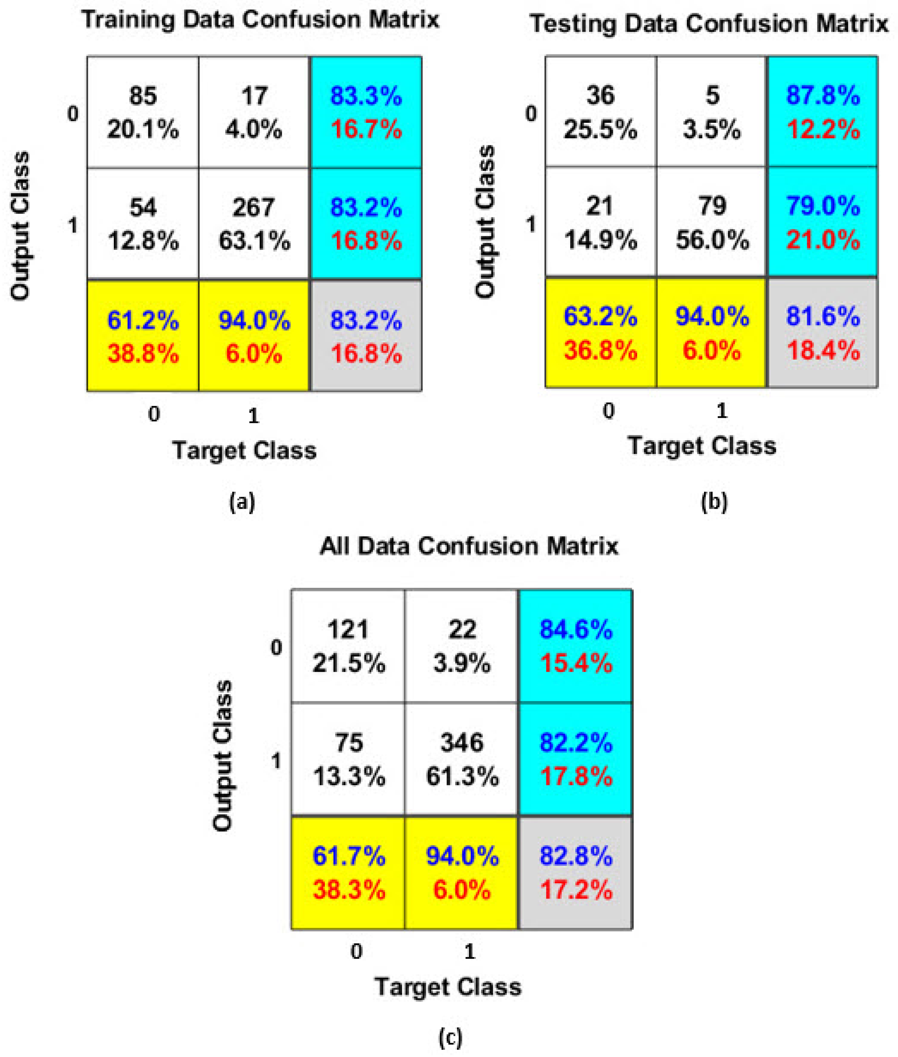
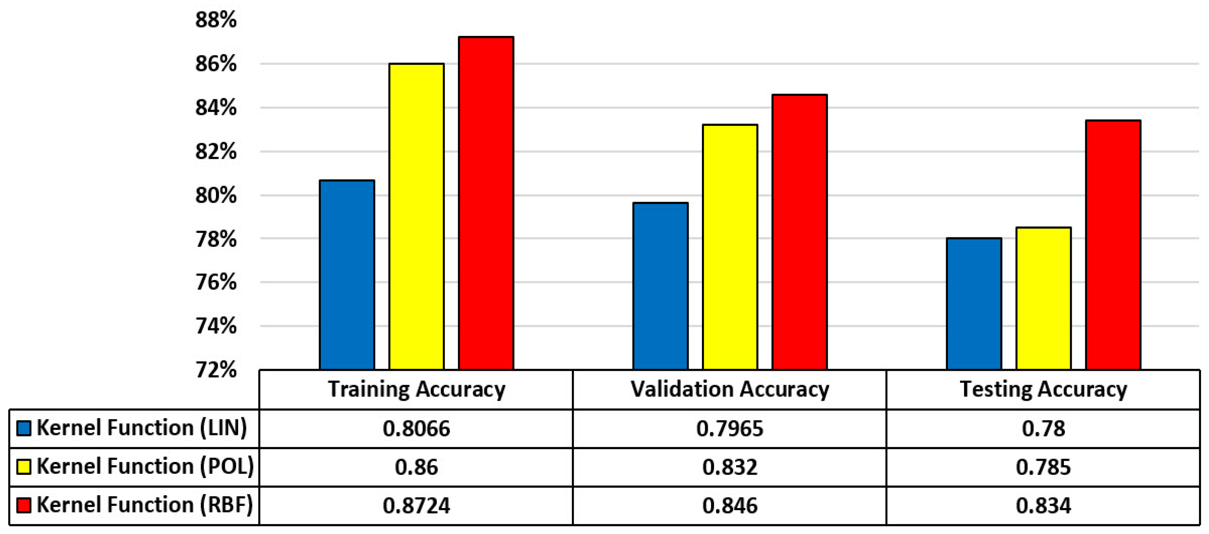
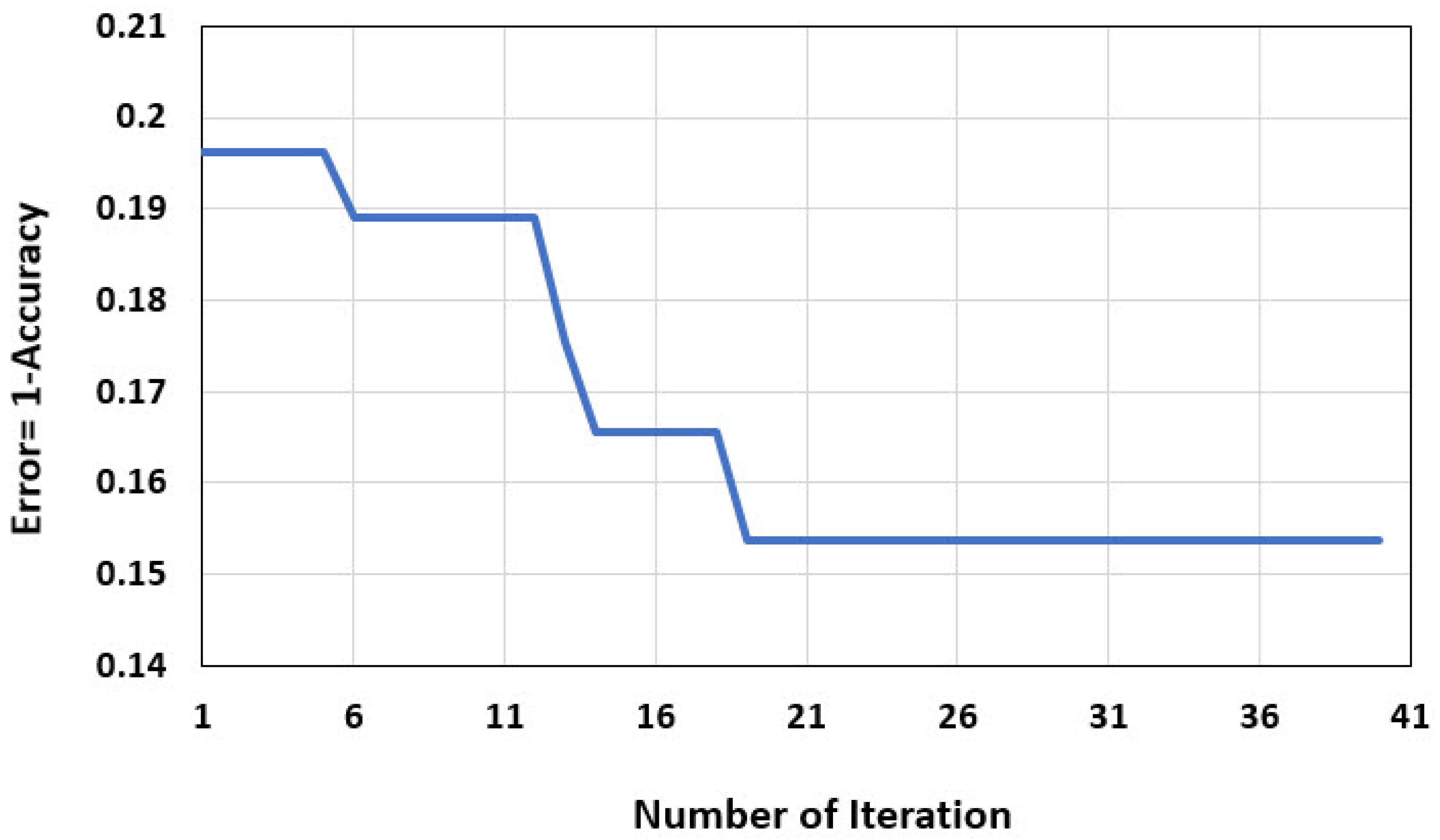
4.2. GOA-SVM Modeling

GOA and SVM were combined to develop a predictive model in the MATLAB environment. The GOA algorithm was used to optimize some parameters of the SVM so that the SVM model shows the highest performance. In the GOA-SVM modeling of this study, the same datasets performed in the analysis of GMDH were used. For modeling, 75% of the dataset (423 data) is randomly defined as the training dataset, and the remaining 25% (141 data) is considered as the testing dataset [105]. Like modeling with the GMDH algorithm, the two classes were considered for all data with labels, including “0” and “1”. To develop and optimize the parameters of the SVM model by the GOA, the control parameters of the GOA must be determined, which play an important role in the rapid and appropriate convergence of the model. Although there are no specific relationships to determine these parameters, based on previous studies and experts’ opinions, a range was determined for each of them, such as the number of grasshopper populations (5, 10, 15, 20, 30, and 40) and the number of iterations (10, 20, 40, 50, and 100). Then, the most appropriate ones were selected by a trial-and-error approach [107].
Moreover, to further evaluate the model, k-fold cross-validation was used, in which the data were subdivided into K subsets. In this system, one of them was used at each time for validation, while the other K − 1 was applied for training. This procedure was carried out K times, with each data set being used exactly once for training and once for validation. Finally, the average result of this K validation was chosen as the final estimate. There is no specific method for determining the amount of k-fold, and it is determined according to the number of data and the opinion of experts. Hence, k-fold was considered to be equal to 3 in this study [107]. In addition, the three different types of kernel functions, including RBF, POL, and LIN, were used. According to the number of control parameters, 30 models were built for each kernel function of GOA-SVM. That means, in total, 90 models were made for GOA-SVM. Preliminary analyses were performed, and a comparison of the performance indicators for the best-developed models with three different kernels is shown in Figure 5.
Although the GOA algorithm was able to train SVM very well with different kernels, according to Figure 5, it is clear that the best-developed model with an RBF kernel had the highest degree of accuracy in training, validation, and testing in comparison with the POL and LIN kernel functions. Therefore, the best developed GOA-SVM model is considered with the RBF kernel function and the optimal control parameters of the model are shown in Table 6. Moreover, the value of error in each iteration was calculated based on Equation (25), and the result is indicated in Figure 6. According to Figure 6, modeling started with an error of about 0.195 and had different values until the 18th iteration, reaching 0.153 in the 19th iteration, which remained constant until the last iteration (40th). The obtained values of accuracy and error indicated the proper convergence of the model.

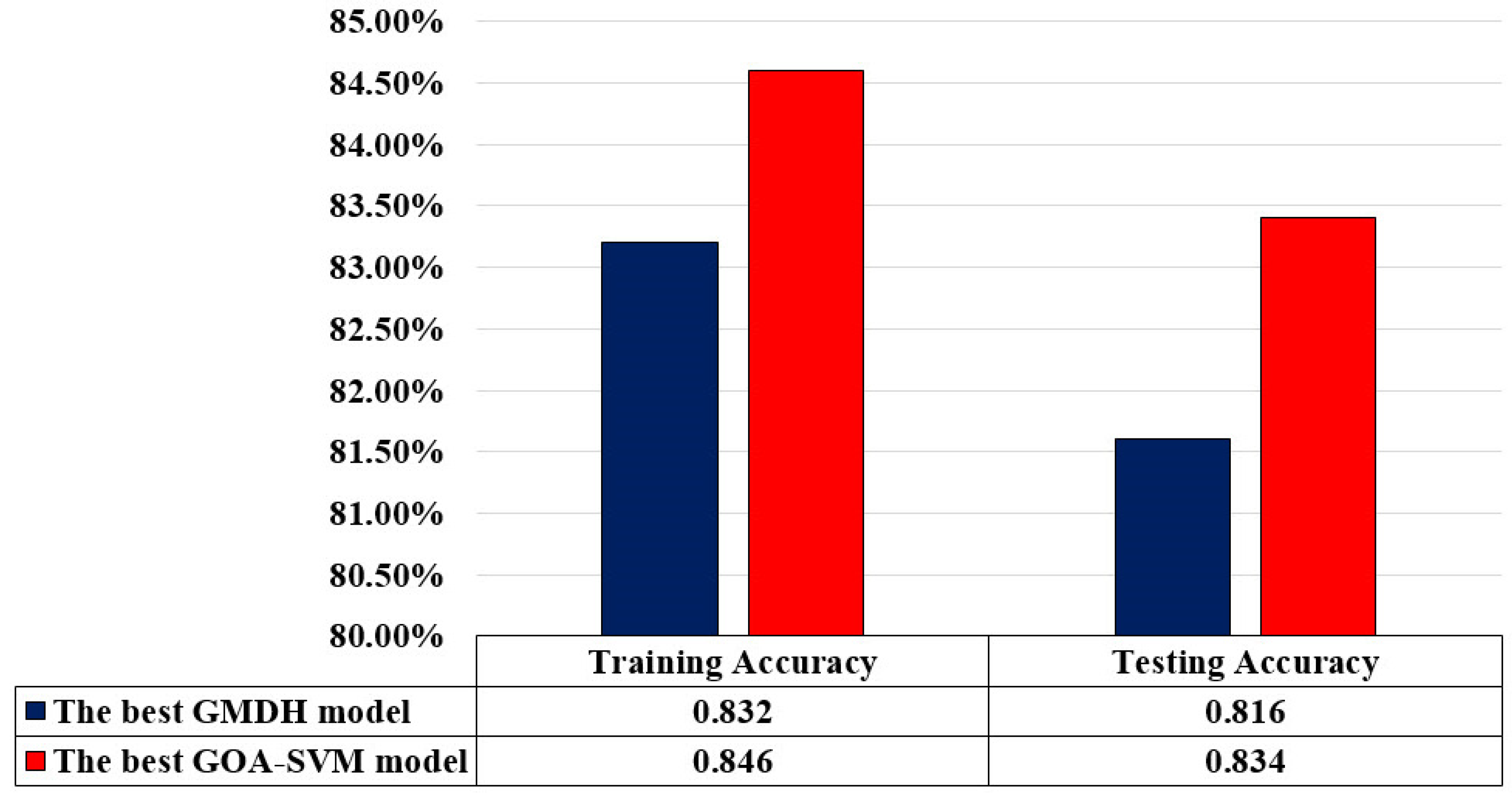
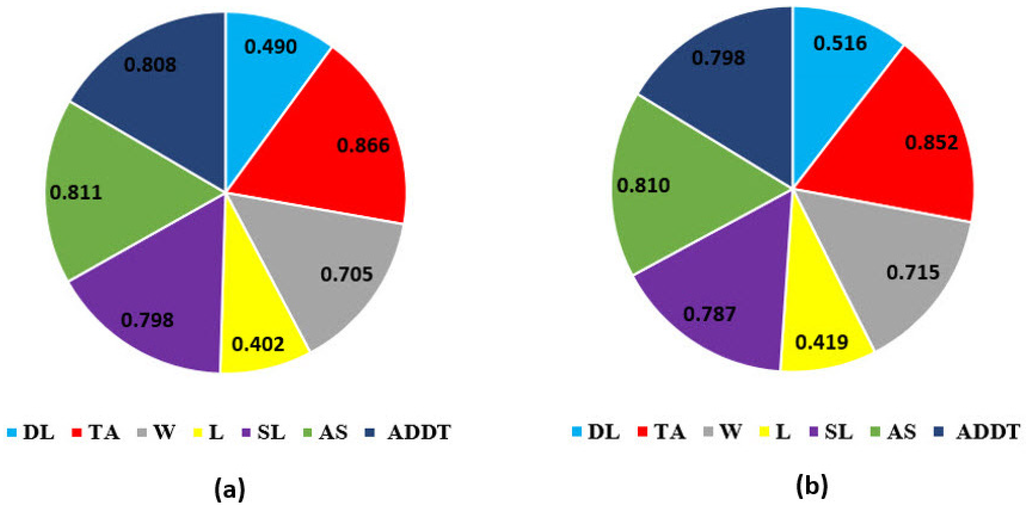
4.3. Comparison of Models’ Performance and Sensitivity Analysis

Each year, many people pass away due to road traffic accidents. Therefore, knowing the impact of various contributing factors on road accidents and taking the necessary measures to reduce accidents can significantly increase the level of road safety. This research employed two machine learning methods, namely GMDH-type neural network and GOA-SVM, to conduct the binary classification modeling. Based on the accuracy of the modeling performance, the best GMDH and GOA-SVM models were chosen after multiple modeling. A comparison was made between the best model of GMDH and the best model of GOA-SVM based on the accuracy of training and testing that is shown in Figure 7. According to the explanations in the previous section, it should be noted that the value of the validation accuracy model is considered instead of the value of training accuracy in the GOA-SVM model. Hence the value of validation accuracy of the GOA-SVM model should be compared to the value of training accuracy of the GMDH model.
According to Figure 7, the best GOA-SVM model indicated higher performance than the best GMDH model for predicting the number of accidents by 84.6% and 83.4% for training and testing accuracies, in comparison with 83.2% and 81.6% for training and testing accuracies, respectively. Although it is worth mentioning that both models had acceptable degrees of accuracy and robustness, it can be concluded that they are reliable systems of modeling for predicting the number of vehicles involved in an accident and can be used as useful tools for modeling road safety involved in transportation engineering.
Road accidents can cause considerable economic and human losses to society. Therefore, assessing the impact of parameters affecting the number of vehicles involved in an accident can provide an in-depth insight for engineers involved in road safety management. A sensitivity analysis was performed to assess the impact of DL, W, TA, L, SL, AS, and AADT on the predicted number of vehicles involved in the accident. This sensitivity analysis is based on the cosine amplitude method according to Equation (26), in which rij is the strength of the relationship, n shows the number of datasets, and xik and yij explain the input variables and the predicted output, correspondingly [108,109].
r i j = k = 1 n ( x i k × y j k ) k = 1 n x i k 2 k = 1 n y i k 2
According to Figure 8, it is clear that the analyses of both models had similar results from the impact of the factors under consideration, which indicates the reliability of the results. Furthermore, the following remarks can be concluded:
-
The type of accident was the most significant factor among other contributing factors that affected the number of vehicles involved in the crashes. In general, certain types of accidents can be caused by a variety of issues, including a lack of traffic signs and poor road quality. The type of accident has an important effect on the number of vehicles involved in an accident.
-
The next factor is the average speed, which can increase the risk of accidents. Some researchers discovered that controlling other factors, such as traffic volume, road geometry, and the number of lanes, can reduce or eliminate the effects of average speed [110,111]. When the average speed is higher, the driver’s response time is shorter, which can lead to an accident. Therefore, it is possible to control the impact of average speed by providing some types of measures, such as improvement to the location of road signs, speed limit enforcement methods, pavement markings, and vertical centerline treatments.
-
The third factor influencing the number of vehicles involved in an accident after the type of accident and the average speed is the annual average daily traffic that plays a key role in the development needs and priorities of road development for transportation planning. Moreover, some studies indicate that increasing the amount of AADT can lead to an increase in the frequency of accidents [112,113]. Therefore, to reduce the effects of AADT on this case study, it is recommended to consider other intercity transportation systems, such as trains, which are being considered in the review of coming urban development plans.
-
The subsequent contributing factor is the speed limit, which has a significant role in the behavior and decisions of drivers. Generally, it is considered that the speed limit is determined by the road conditions. If the speed limit is selected incorrectly on a part of the route and the driver is aware of this error due to the road conditions, they may lose confidence in the speed limits in other sections of the road and increase or decrease the speed based on their interpretation [114,115]. Hence, given the impact of this factor in this case study, it is suggested that a general review be considered in selecting the speed limit for rural roads in Cosenza.
-
Several appropriate studies have been conducted on the relationship between weekdays and accidents [116,117]. In line with national statistics, road accidents are more concentrated on holidays on the road network in Cosenza’s province. In the present study, out of the 564 accidents, 65% (367) occurred on holidays. Due to the geographical location of Cosenza, the amount of traffic on holidays has experienced a relative increase. To reduce the exposure to the risk, the intensification of controls and monitoring of roads during the holidays would mitigate the effect of this factor by increasing police enforcement.
-
Extensive studies have been conducted on the effect of daylight on the number of vehicles involved in accidents, which shows this factor’s high importance. This factor has been given priority in many studies, among other factors [50,118]. The amount of impact this factor has is heavily influenced by its geographic location and road lighting systems. This factor was determined as the sixth most effective factor out of seven factors, and this result was matched with the location and road lighting system of rural roads in Cosenza.
-
The last studied factor was the location that had the most negligible impact on the rate of vehicles involved in an accident, based on the results of both artificial intelligence models. Based on the type of structure of the rural roads in Cosenza, the location has not had much effect on the rate of accidents. Therefore, in future studies on this case study, the effect of this factor can be ignored.
Human behavior is jointly responsible for road accidents, together with the vehicle and the environment (of which the infrastructure is part). It is strictly correlated to the speed and type of accident, and the author’s analysis of the importance and the proposed methodology determined the impacts. Moreover, these two factors have the highest impact compared to other parameters on the rate of vehicles involved in accidents on the rural roads of Cosenza.
Therefore, based on the results obtained and after consulting experts, it can be concluded that several measures, such as improving roadway geometry, pavement markings, and vertical centerline treatments, are the most significant measures that should be considered in reviewing the plan for rural roads in Cosenza. Finally, it should be noted that the presented models with specific structures are location-sensitive and cannot be directly used on other rural roads.

5. Conclusions

The evaluation and analysis of contributing factors affecting the number of vehicles involved in the crashes can lead to a deep understanding of the existing situation and increase road safety by planning and taking a series of necessary measures. Therefore, this study made an attempt to predict the number of vehicles involved in the crashes using the GMDH-type neural network and GOA-SVM methods. This study was accomplished using 564 accident cases from rural roads in Cosenza in southern Italy. Several crash-related parameters, including DL, W, TA, L, SL, AS, and AADT, were set as input variables, and the number of vehicles involved in the crash was considered as the output data. According to each technique’s number of control parameters, 25 models were made for GMDH and 30 models for each kernel function of GOA-SVM, so a total of 90 models were made for GOA-SVM. After modeling, the models for each technique were compared with each other in terms of the model’s performance. Among the binary classification of GMDH models, the 15th model was selected with the highest score, and the GOA-SVM model with RBF kernel function was chosen among the binary classification of GOA-SVM models. In the comparison between the GMDH and GOA-SVM models, the GOA-SVM model had a higher capability for the prediction of the number of vehicles involved in the accident, although the performance of both models indicates that both can be used as useful tools for modeling the number of vehicles involved in an accident in transportation engineering. Consequently, a sensitivity analysis was performed based on the results obtained from both models. In both models, the type of accident and location had the highest and lowest impact compared to other parameters on the rate of vehicles involved in accidents on the rural roads of Cosenza, respectively. The results of this study showed the role of humans in causing accidents as the most contributing factor in road safety, which was fully consistent with previous studies in this field. As a result, it is recommended that organizations concerned with road safety, in addition to taking the required steps to enhance road condition, establish a long-term strategy for raising awareness and assessing driver performance.
For future work, it is recommended to examine other factors that can impact the number of vehicles involved in an accident, such as the age of drivers, the age of cars, gender, and the geometry of roads.

Author Contributions

Conceptualization, G.G. and S.S.H. (Sina Shaffiee Haghshenas); methodology, S.S.H. (Sina Shaffiee Haghshenas) and S.S.H. (Sami Shaffiee Haghshenas); software, S.S.H. (Sina Shaffiee Haghshenas); formal analysis, S.S.H. (Sina Shaffiee Haghshenas); investigation, S.S.H. (Sina Shaffiee Haghshenas) and S.S.H. (Sami Shaffiee Haghshenas); resources, G.G., V.A. and A.V.; writing—original draft preparation, S.S.H. (Sina Shaffiee Haghshenas); writing—review and editing, G.G., S.S.H. (Sina Shaffiee Haghshenas), S.S.H. (Sami Shaffiee Haghshenas), V.A., Y.P. and Z.W.G.; supervision, G.G., V.A., A.V., Y.P. and Z.W.G. All authors have read and agreed to the published version of the manuscript.

Funding

This research received no external funding.

Institutional Review Board Statement

Not applicable.

Informed Consent Statement

Not applicable.

Data Availability Statement

Not applicable.

Acknowledgments

We would like to express our deepest thanks to Mahdi Ghaem for his excellent advice.

Conflicts of Interest

The authors declare no conflict of interest.

References

  1. Nordfjærn, T.; Rundmo, T. Road traffic safety beliefs and driver behaviors among personality subtypes of drivers in the Norwegian population. Traffic Inj. Prev. 2013, 14, 690–696. [Google Scholar] [CrossRef] [PubMed]
  2. Ellison, A.B.; Greaves, S.P.; Bliemer, M.C. Driver behaviour profiles for road safety analysis. Accid. Anal. Prev. 2015, 76, 118–132. [Google Scholar] [CrossRef] [PubMed]
  3. Scott-Parker, B. Emotions, behaviour, and the adolescent driver: A literature review. Transp. Res. F Traffic Psychol. Behav. 2017, 50, 1–37. [Google Scholar] [CrossRef]
  4. Farooq, D.; Moslem, S.; Duleba, S. Evaluation of driver behavior criteria for evolution of sustainable traffic safety. Sustainability 2019, 11, 3142. [Google Scholar] [CrossRef] [Green Version]
  5. Farooq, D.; Juhasz, J. Statistical Evaluation of Risky Driver Behavior Factors That Influence Road Safety Based on Drivers Age and Driving Experience in Budapest and Islamabad. Eur. Transp. 2020, 80, 1–18. [Google Scholar] [CrossRef]
  6. Rosli, N.; Ambak, K.; Shahidan, N.N.; Sukor, N.S.A.; Osman, S.; Yei, L.S. Driving behaviour of elderly drivers in Malaysia. Int. J. Integr. Eng. 2020, 12, 268–277. [Google Scholar] [CrossRef]
  7. Alonso, B.; Astarita, V.; Dell’Olio, L.; Giofrè, V.P.; Guido, G.; Marino, M.; Sommario, W.; Vitale, A. Validation of simulated safety indicators with traffic crash data. Sustainability 2020, 12, 925. [Google Scholar] [CrossRef] [Green Version]
  8. Christoforou, Z.D.; Karlaftis, M.G.; Yannis, G. Heavy vehicle age and road safety. In Proceedings of the Institution of Civil Engineers-Transport, London, UK, 22–23 November 2010; Thomas Telford Ltd.: London, UK, 2010; Volume 163, pp. 41–48. [Google Scholar]
  9. Russo, F.; Biancardo, S.A.; Dell’Acqua, G. Road safety from the perspective of driver gender and age as related to the injury crash frequency and road scenario. Traffic Inj. Prev. 2014, 15, 25–33. [Google Scholar] [CrossRef] [Green Version]
  10. Kim, S.; Kim, J.K. Road safety for an aged society: Compliance with traffic regulations, knowledge about traffic regulations, and risk factors of older drivers. Transp. Res. Rec. 2017, 2660, 15–21. [Google Scholar] [CrossRef]
  11. Casado-Sanz, N.; Guirao, B. Analysis of the impact of population ageing and territorial factors on crosstown roads safety: The Spanish case study. Transp. Res. Procedia 2018, 33, 283–290. [Google Scholar] [CrossRef]
  12. Török, Á. A Novel Approach in Evaluating the Impact of Vehicle Age on Road Safety. Promet Traffic Transp. 2020, 32, 789–796. [Google Scholar] [CrossRef]
  13. Lyon, C.; Mayhew, D.; Granie, M.A.; Robertson, R.; Vanlaar, W.; Woods-Fry, H.; Thevenetb, C.; Furian, G.; Soteropoulos, A. Age and road safety performance: Focusing on elderly and young drivers. IATSS Res. 2020, 44, 212–219. [Google Scholar] [CrossRef]
  14. Theofilatos, A.; Yannis, G. A review of the effect of traffic and weather characteristics on road safety. Accid. Anal. Prev. 2014, 72, 244–256. [Google Scholar] [CrossRef] [PubMed]
  15. Lazarev, Y.; Medres, C.; Raty, J.; Bondarenko, A. Method of Assessment and Prediction of Temperature Conditions of Roadway Surfacing as a Factor of the Road Safety. Transp. Res. Procedia 2017, 20, 393–400. [Google Scholar] [CrossRef]
  16. Malin, F.; Norros, I.; Innamaa, S. Accident risk of road and weather conditions on different road types. Accid. Anal. Prev. 2018, 122, 181–188. [Google Scholar] [CrossRef]
  17. Ivajnšič, D.; Horvat, N.; Žiberna, I.; Kotnik, E.; Davidović, D. Revealing the Spatial Pattern of Weather-Related Road Traffic Crashes in Slovenia. Appl. Sci. 2021, 11, 6506. [Google Scholar] [CrossRef]
  18. Abdella, G.M.; Shaaban, K. Modeling the impact of weather conditions on pedestrian injury counts using LASSO-based poisson model. Arab. J. Sci. Eng. 2021, 46, 4719–4730. [Google Scholar] [CrossRef]
  19. Bajwa, S.; Warita, M.; Kuwahara, M. Effects of road geometry, weather and traffic flow on road safety. In Proceedings of the 15th International Conference of Hong Kong Society for Transportation Study, Hong Kong, China, 11–14 December 2010; pp. 773–780. [Google Scholar]
  20. Orfila, O.; Coiret, A.; Do, M.; Mammar, S. Modeling of dynamic vehicle–road interactions for safety-related road evaluation. Accid. Anal. Prev. 2010, 42, 1736–1743. [Google Scholar] [CrossRef]
  21. Alian, S.; Baker, R.; Wood, S. Rural casualty crashes on the Kings Highway: A new approach for road safety studies. Accid. Anal. Prev. 2016, 95, 8–19. [Google Scholar] [CrossRef]
  22. Ewan, L.; Al-Kaisy, A.; Hossain, F. Safety Effects of Road Geometry and Roadside Features on Low-Volume Roads in Oregon. Transp. Res. Rec. 2016, 2580, 47–55. [Google Scholar] [CrossRef] [Green Version]
  23. Gooch, J.P.; Gayah, V.V.; Donnell, E.T. Quantifying the safety effects of horizontal curves on two-way, two-lane rural roads. Accid. Anal. Prev. 2016, 92, 71–81. [Google Scholar] [CrossRef] [PubMed]
  24. Roslak, J.; Wallaschek, J. Active lighting systems for improved road safety. In Proceedings of the IEEE Intelligent Vehicles Symposium, Parma, Italy, 14–17 June 2004; pp. 682–685. [Google Scholar]
  25. Magar, S.G. Adaptive Front Light Systems of Vehicle for Road Safety. In Proceedings of the 2015 International Conference on Computing Communication Control and Automation, Pune, India, 6–27 February 2015; pp. 551–554. [Google Scholar]
  26. Aldulaimi, M.; AmadorJimenez, L. 759 Road lighting and safety: A pilot study of Arthabaska region. Inj. Prev. 2016, 22, A272. [Google Scholar] [CrossRef] [Green Version]
  27. Tetervenoks, O.; Avotins, A.; Fedorjana, N.; Kluga, A.; Krasts, V. Potential Role of Street Lighting System for Safety Enhancement on the Roads in Future. In Proceedings of the 2019 IEEE 60th International Scientific Conference on Power and Electrical Engineering of Riga Technical University (RTUCON), Riga, Latvia, 7–9 October 2019; pp. 1–5. [Google Scholar]
  28. Liu, J.; Li, J.; Wang, K.; Zhao, J.; Cong, H.; He, P. Exploring factors affecting the severity of night-time vehicle accidents under low illumination conditions. Adv. Mech. Eng. 2019, 11, 1687814019840940. [Google Scholar] [CrossRef]
  29. Saljoqi, M.; Behnood, H.R.; Mirbaha, B. Developing the crash modification model for urban street lighting. Innov. Infrastruct. Solut. 2021, 6, 59. [Google Scholar] [CrossRef]
  30. Siliquini, R.; Piat, S.C.; Alonso, F.; Druart, A.; Kedzia, M.; Mollica, A.; Siliquini, V.; Vankov, D.; Villerusa, A.; Manzoli, L.; et al. A European study on alcohol and drug use among young drivers: The TEND by Night study design and methodology. BMC Public Health 2010, 10, 205. [Google Scholar] [CrossRef] [Green Version]
  31. Alonso, F.; Esteban, C.; Useche, S.A.; Faus, M. Smoking while driving: Frequency, motives, perceived risk and punishment. World J. Prev. Med. 2017, 5, 1–9. [Google Scholar]
  32. Zou, X.; Yue, W.L.; Vu, H.L. Visualization and analysis of mapping knowledge domain of road safety studies. Accid. Anal. Prev. 2018, 118, 131–145. [Google Scholar] [CrossRef]
  33. Elvik, R.; Vadeby, A.; Hels, T.; van Schagen, I. Updated estimates of the relationship between speed and road safety at the aggregate and individual levels. Accid. Anal. Prev. 2019, 123, 114–122. [Google Scholar] [CrossRef]
  34. Gichaga, F.J. The impact of road improvements on road safety and related characteristics. IATSS Res. 2017, 40, 72–75. [Google Scholar] [CrossRef] [Green Version]
  35. Sager, L. Estimating the effect of air pollution on road safety using atmospheric temperature inversions. J. Environ. Econ. Manag. 2019, 98, 102250. [Google Scholar] [CrossRef]
  36. Mahmud, S.M.S.; Ferreira, L.; Tavassoli, A. Traditional approaches to Traffic Safety Evaluation (TSE): Application challenges and future directions. In Proceedings of the 11th Asia Pacific Transportation Development Conference and 29th ICTPA Annual Conference, Hsinchu, Taiwan, 27–29 May 2016; pp. 242–262. [Google Scholar]
  37. Zheng, L.; Ismail, K.; Sayed, T.; Fatema, T. Bivariate extreme value modeling for road safety estimation. Accid. Anal. Prev. 2018, 120, 83–91. [Google Scholar] [CrossRef] [PubMed]
  38. Wang, C.; Xu, C.; Dai, Y. A crash prediction method based on bivariate extreme value theory and video-based vehicle trajectory data. Accid. Anal. Prev. 2019, 123, 365–373. [Google Scholar] [CrossRef] [PubMed]
  39. Zheng, L.; Sayed, T.; Mannering, F. Modeling traffic conflicts for use in road safety analysis: A review of analytic methods and future directions. Anal. Methods Accid. Res. 2020, 29, 100142. [Google Scholar] [CrossRef]
  40. Jamal, A.; Rahman, M.T.; Al-Ahmadi, H.M.; Mansoor, U. The Dilemma of Road Safety in the Eastern Province of Saudi Arabia: Consequences and Prevention Strategies. Int. J. Environ. Res. Public Health 2019, 17, 157. [Google Scholar] [CrossRef] [PubMed] [Green Version]
  41. Mussone, L.; Ferrari, A.; Oneta, M. An analysis of urban collisions using an artificial intelligence model. Accid. Anal. Prev. 1999, 31, 705–718. [Google Scholar] [CrossRef]
  42. Halim, Z.; Kalsoom, R.; Bashir, S.; Abbas, G. Artificial intelligence techniques for driving safety and vehicle crash prediction. Artif. Intell. Rev. 2016, 46, 351–387. [Google Scholar] [CrossRef]
  43. Castro, Y.; Kim, Y.J. Data mining on road safety: Factor assessment on vehicle accidents using classification models. Int. J. Crashworthiness 2015, 21, 104–111. [Google Scholar] [CrossRef]
  44. De Luca, M. A comparison between prediction power of artificial neural networks and multivariate analysis in road safety management. Transport 2017, 32, 379–385. [Google Scholar] [CrossRef] [Green Version]
  45. Shah, S.A.R.; Brijs, T.; Ahmad, N.; Pirdavani, A.; Shen, Y.; Basheer, M.A. Road safety risk evaluation using gis-based data envelopment analysis—Artificial neural networks approach. Appl. Sci. 2017, 7, 886. [Google Scholar] [CrossRef] [Green Version]
  46. Liu, M.; Wu, Z.; Chen, Y.; Zhang, X. Utilizing Decision Tree Method and ANFIS to Explore Real-Time Crash Risk for Urban Freeways. In Proceedings of the CICTP 2020, Xi’an, China, 14–16 August 2020; pp. 2495–2508. [Google Scholar]
  47. Guido, G.; Haghshenas, S.; Haghshenas, S.; Vitale, A.; Gallelli, V.; Astarita, V. Development of a Binary Classification Model to Assess Safety in Transportation Systems Using GMDH-Type Neural Network Algorithm. Sustainability 2020, 12, 6735. [Google Scholar] [CrossRef]
  48. Mokhtarimousavi, S.; Anderson, J.C.; Hadi, M.; Azizinamini, A. A temporal investigation of crash severity factors in worker-involved work zone crashes: Random parameters and machine learning approaches. Transp. Res. Interdiscip. Perspect. 2021, 10, 100378. [Google Scholar] [CrossRef]
  49. Kitali, A.E.; Mokhtarimousavi, S.; Kadeha, C.; Alluri, P. Severity analysis of crashes on express lane facilities using support vector machine model trained by firefly algorithm. Traffic Inj. Prev. 2020, 22, 79–84. [Google Scholar] [CrossRef] [PubMed]
  50. Xu, Y.; Ye, Z.; Wang, Y.; Wang, C.; Sun, C. Evaluating the influence of road lighting on traffic safety at accesses using an artificial neural network. Traffic Inj. Prev. 2018, 19, 601–606. [Google Scholar] [CrossRef] [PubMed]
  51. Amiri, A.M.; Sadri, A.; Nadimi, N.; Shams, M. A comparison between Artificial Neural Network and Hybrid Intelligent Genetic Algorithm in predicting the severity of fixed object crashes among elderly drivers. Accid. Anal. Prev. 2020, 138, 105468. [Google Scholar] [CrossRef]
  52. Guido, G.; Haghshenas, S.; Haghshenas, S.; Vitale, A.; Astarita, V.; Haghshenas, A. Feasibility of Stochastic Models for Evaluation of Potential Factors for Safety: A Case Study in Southern Italy. Sustainability 2020, 12, 7541. [Google Scholar] [CrossRef]
  53. Shiran, G.; Imaninasab, R.; Khayamim, R. Crash Severity Analysis of Highways Based on Multinomial Logistic Regression Model, Decision Tree Techniques, and Artificial Neural Network: A Modeling Comparison. Sustainability 2021, 13, 5670. [Google Scholar] [CrossRef]
  54. Mussone, L.; Bassani, M.; Masci, P. Analysis of factors affecting the severity of crashes in urban road intersections. Accid. Anal. Prev. 2017, 103, 112–122. [Google Scholar] [CrossRef]
  55. Ministero delle Infrastrutture e dei Trasporti. Nuovo Codice della Strada, Decreto Legislativo N. 285 del 30/4/1992, G.U. n. 114 del 18/5/1992. Gazzetta Ufficiale, 1992. [Google Scholar]
  56. Ministero delle Infrastrutture e dei Trasporti. Disposizioni urgenti per la sicurezza della circolazione dei veicoli e di specifiche categorie di utenti, Modifiche al Nuovo Codice della Strada, Decreto Legislativo n.121 del 10/9/2021, G.U. n. 267 del 9/9/2021. Gazzetta Ufficiale, 2021. [Google Scholar]
  57. Pan, G.; Fu, L.; Thakali, L. Development of a global road safety performance function using deep neural networks. Int. J. Transp. Sci. Technol. 2017, 6, 159–173. [Google Scholar] [CrossRef]
  58. Peng, Z.; Gao, S.; Li, Z.; Xiao, B.; Qian, Y. Vehicle Safety Improvement through Deep Learning and Mobile Sensing. IEEE Netw. 2018, 32, 28–33. [Google Scholar] [CrossRef]
  59. Silva, P.B.; Andrade, M.; Ferreira, S. Machine learning applied to road safety modeling: A systematic literature review. J. Traffic Transp. Eng. 2020, 7, 775–790. [Google Scholar] [CrossRef]
  60. Hernández, H.; Alberdi, E.; Pérez-Acebo, H.; Álvarez, I.; García, M.; Eguia, I.; Fernández, K. Managing Traffic Data through Clustering and Radial Basis Functions. Sustainability 2021, 13, 2846. [Google Scholar] [CrossRef]
  61. Amiri, A.M.; Naderi, K.; Cooper, J.F.; Nadimi, N. Evaluating the impact of socio-economic contributing factors of cities in California on their traffic safety condition. J. Transp. Health 2021, 20, 101010. [Google Scholar] [CrossRef]
  62. Jamal, A.; Zahid, M.; Tauhidur Rahman, M.; Al-Ahmadi, H.M.; Almoshaogeh, M.; Farooq, D.; Ahmad, M. Injury severity prediction of traffic crashes with ensemble machine learning techniques: A comparative study. Int. J. Inj. Contr. Saf. Promot. 2021, 28, 408–427. [Google Scholar] [CrossRef] [PubMed]
  63. Hosseinzadeh, A.; Moeinaddini, A.; Ghasemzadeh, A. Investigating factors affecting severity of large truck-involved crashes: Comparison of the SVM and random parameter logit model. J. Saf. Res. 2021, 77, 151–160. [Google Scholar] [CrossRef] [PubMed]
  64. Tehrany, M.S.; Pradhan, B.; Jebur, M.N. Flood susceptibility mapping using a novel ensemble weights-of-evidence and support vector machine models in GIS. J. Hydrol. 2014, 512, 332–343. [Google Scholar] [CrossRef]
  65. Jahed Armaghani, D.; Asteris, P.G.; Askarian, B.; Hasanipanah, M.; Tarinejad, R.; Huynh, V.V. Examining hybrid and single SVM models with different kernels to predict rock brittleness. Sustainability 2020, 12, 2229. [Google Scholar] [CrossRef] [Green Version]
  66. Mikaeil, R.; Haghshenas, S.S.; Ozcelik, Y.; Gharehgheshlagh, H.H. Performance evaluation of adaptive neuro-fuzzy inference system and group method of data handling-type neural network for estimating wear rate of diamond wire saw. Geotech. Geol. Eng. 2018, 36, 3779–3791. [Google Scholar] [CrossRef]
  67. Dormishi, A.R.; Ataei, M.; Khaloo Kakaie, R.; Mikaeil, R.; Shaffiee Haghshenas, S. Performance evaluation of gang saw using hybrid ANFIS-DE and hybrid ANFIS-PSO algorithms. JME 2019, 10, 543–557. [Google Scholar]
  68. Naderpour, H.; Mirrashid, M. Moment capacity estimation of spirally reinforced concrete columns using ANFIS. Complex Intell. Syst. 2019, 6, 97–107. [Google Scholar] [CrossRef] [Green Version]
  69. Shirani Faradonbeh, R.; Shaffiee Haghshenas, S.; Taheri, A.; Mikaeil, R. Application of self-organizing map and fuzzy c-mean techniques for rockburst clustering in deep underground projects. Neural Comput. Appl. 2019, 32, 8545–8559. [Google Scholar] [CrossRef]
  70. Noori, A.M.; Mikaeil, R.; Mokhtarian, M.; Haghshenas, S.S.; Foroughi, M. Feasibility of Intelligent Models for Prediction of Utilization Factor of TBM. Geotech. Geol. Eng. 2020, 38, 3125–3143. [Google Scholar] [CrossRef]
  71. Golafshani, E.M.; Behnood, A. Predicting the mechanical properties of sustainable concrete containing waste foundry sand using multi-objective ANN approach. Constr. Build. Mater. 2021, 291, 123314. [Google Scholar] [CrossRef]
  72. Ivakhnenko, A.G. Polynomial Theory of Complex Systems. IEEE Trans. Syst. Man Cybern. 1971, SMC-1, 364–378. [Google Scholar] [CrossRef] [Green Version]
  73. Sezavar, R.; Shafabakhsh, G.; Mirabdolazimi, S.M. New model of moisture susceptibility of nano silica-modified asphalt concrete using GMDH algorithm. Constr. Build Mater. 2019, 211, 528–538. [Google Scholar] [CrossRef]
  74. Dag, O.; Kasikci, M.; Karabulut, E.; Alpar, R. Diverse classifiers ensemble based on GMDH-type neural network algorithm for binary classification. Commun. Stat. Simul. Comput. 2019, 1–17. [Google Scholar] [CrossRef]
  75. Armaghani, D.J.; Hasanipanah, M.; Amnieh, H.B.; Bui, D.T.; Mehrabi, P.; Khorami, M. Development of a novel hybrid intelligent model for solving engineering problems using GS-GMDH algorithm. Eng. Comput. 2019, 36, 1379–1391. [Google Scholar] [CrossRef]
  76. Harandizadeh, H.; Armaghani, D.J.; Mohamad, E.T. Development of fuzzy-GMDH model optimized by GSA to predict rock tensile strength based on experimental datasets. Neural Comput. Appl. 2020, 32, 14047–14067. [Google Scholar] [CrossRef]
  77. Jeddi, S.; Sharifian, S. A hybrid wavelet decomposer and GMDH-ELM ensemble model for Network function virtualization workload forecasting in cloud computing. Appl. Soft Comput. 2019, 88, 105940. [Google Scholar] [CrossRef]
  78. Morosini, A.F.; Haghshenas, S.S.; Geem, Z.W. Development of a Binary Model for Evaluating Water Distribution Systems by a Pressure Driven Analysis (PDA) Approach. Appl. Sci. 2020, 10, 3029. [Google Scholar] [CrossRef]
  79. Khandezamin, Z.; Naderan, M.; Rashti, M.J. Detection and classification of breast cancer using logistic regression feature selection and GMDH classifier. J. Biomed. Inform. 2020, 111, 103591. [Google Scholar] [CrossRef]
  80. Fiorini Morosini, A.; Shaffiee Haghshenas, S.; Shaffiee Haghshenas, S.; Choi, D.Y.; Geem, Z.W. Sensitivity Analysis for Performance Evaluation of a Real Water Distribution System by a Pressure Driven Analysis Approach and Artificial Intelligence Method. Water 2021, 13, 1116. [Google Scholar] [CrossRef]
  81. Pusat, S.; Akkaya, A.V. Explicit equation derivation for predicting coal moisture content in convective drying process by GMDH-type neural network. Int. J. Coal Prep. 2020, 1–14. [Google Scholar] [CrossRef]
  82. Vissol-Gaudin, E.; Kotsialos, A.; Groves, C.; Pearson, C.; Zeze, D.A.; Petty, M.C. Computing based on material training: Application to binary classification problems. In Proceedings of the 2017 IEEE International Conference on Rebooting Computing (ICRC), Washington, DC, USA, 8–9 November 2017; pp. 1–8. [Google Scholar]
  83. Li, D.; Armaghani, D.J.; Zhou, J.; Lai, S.H.; Hasanipanah, M. A GMDH predictive model to predict rock material strength using three non-destructive tests. J. Nondestruct. Eval. 2020, 39, 81. [Google Scholar] [CrossRef]
  84. Cortes, C.; Vapnik, V. Support-vector networks. Mach. Learn. 1985, 20, 273–297. [Google Scholar] [CrossRef]
  85. Chen, W.H.; Hsu, S.H.; Shen, H.P. Application of SVM and ANN for intrusion detection. Comput. Oper. Res. 2005, 32, 2617–2634. [Google Scholar] [CrossRef]
  86. Yan, X.; Jia, M. A novel optimized SVM classification algorithm with multi-domain feature and its application to fault diagnosis of rolling bearing. Neural. Comput. Appl. 2018, 313, 47–64. [Google Scholar] [CrossRef]
  87. Zhou, S.; Chu, X.; Cao, S.; Liu, X.; Zhou, Y. Prediction of the ground temperature with ANN, LS-SVM and fuzzy LS-SVM for GSHP application. Geothermics 2019, 84, 101757. [Google Scholar] [CrossRef]
  88. Maldonado, S.; López, J.; Jimenez-Molina, A.; Lira, H. Simultaneous feature selection and heterogeneity control for SVM classification: An application to mental workload assessment. Expert Syst. Appl. 2020, 143, 112988. [Google Scholar] [CrossRef]
  89. Zeng, J.; Roussis, P.C.; Mohammed, A.S.; Maraveas, C.; Fatemi, S.A.; Armaghani, D.J.; Asteris, P.G. Prediction of Peak Particle Velocity Caused by Blasting through the Combinations of Boosted-CHAID and SVM Models with Various Kernels. Appl. Sci. 2021, 11, 3705. [Google Scholar] [CrossRef]
  90. Zhou, J.; Qiu, Y.; Zhu, S.; Armaghani, D.J.; Li, C.; Nguyen, H.; Yagiz, S. Optimization of support vector machine through the use of metaheuristic algorithms in forecasting TBM advance rate. Eng. Appl. Artif. Intell. 2021, 97, 104015. [Google Scholar] [CrossRef]
  91. Mikaeil, R.; Haghshenas, S.S.; Hoseinie, S.H. Rock penetrability classification using artificial bee colony (ABC) algorithm and self-organizing map. Geotech. Geol. Eng. 2018, 36, 1309–1318. [Google Scholar] [CrossRef]
  92. Salemi, A.; Mikaeil, R.; Haghshenas, S.S. Integration of finite difference method and genetic algorithm to seismic analysis of circular shallow tunnels (Case study: Tabriz urban railway tunnels). KSCE J. Civ. Eng. 2018, 22, 1978–1990. [Google Scholar] [CrossRef]
  93. Aryafar, A.; Mikaeil, R.; Haghshenas, S.S.; Haghshenas, S.S. Application of metaheuristic algorithms to optimal clustering of sawing machine vibration. MEAS 2018, 124, 20–31. [Google Scholar] [CrossRef]
  94. Mikaeil, R.; Haghshenas, S.S.; Sedaghati, Z. Geotechnical risk evaluation of tunneling projects using optimization techniques (case study: The second part of Emamzade Hashem tunnel). Nat. Hazards 2019, 97, 1099–1113. [Google Scholar] [CrossRef]
  95. Mikaeil, R.; Bakhshinezhad, H.; Haghshenas, S.S.; Ataei, M. Stability analysis of tunnel support systems using numerical and intelligent simulations (case study: Kouhin Tunnel of Qazvin-Rasht Railway). Rud. Geol. Naft. Zb. 2019, 34, 1–10. [Google Scholar] [CrossRef] [Green Version]
  96. Haghshenas, S.S.; Faradonbeh, R.S.; Mikaeil, R.; Haghshenas, S.S.; Taheri, A.; Saghatforoush, A.; Dormishi, A. A new conventional criterion for the performance evaluation of gang saw machines. MEAS 2019, 46, 159–170. [Google Scholar] [CrossRef]
  97. Saremi, S.; Mirjalili, S.; Lewis, A. Grasshopper optimisation algorithm: Theory and application. Adv. Eng. Softw. 2017, 105, 30–47. [Google Scholar] [CrossRef] [Green Version]
  98. Mafarja, M.; Aljarah, I.; Faris, H.; Hammouri, A.I.; Ala’M, A.Z.; Mirjalili, S. Binary grasshopper optimisation algorithm approaches for feature selection problems. Expert Syst. Appl. 2019, 117, 267–286. [Google Scholar] [CrossRef]
  99. Saxena, A. A comprehensive study of chaos embedded bridging mechanisms and crossover operators for grasshopper optimisation algorithm. Expert Syst. Appl. 2019, 132, 166–188. [Google Scholar] [CrossRef]
  100. Pan, J.S.; Wang, X.; Chu, S.C.; Nguyen, T.T. A multi-group grasshopper optimisation algorithm for application in capacitated vehicle routing problem. Pattern Recognit. 2020, 4, 41–56. [Google Scholar]
  101. Goodarzizad, P.; Mohammadi Golafshani, E.; Arashpour, M. Predicting the construction labour productivity using artificial neural network and grasshopper optimisation algorithm. Int. J. Constr. Manag. 2021, 1–17. [Google Scholar] [CrossRef]
  102. Meraihi, Y.; Gabis, A.B.; Mirjalili, S.; Ramdane-Cherif, A. Grasshopper optimization algorithm: Theory, variants, and applications. IEEE Access 2021, 9, 50001–50024. [Google Scholar] [CrossRef]
  103. Nelson, M.M.; Illingworth, W.T. A Practical Guide to Neural Nets, Addison-Wesley; Addison-Wesley Longman Publishing Co., Inc.: Reading, MA, USA, 1991. [Google Scholar]
  104. Swingler, K. Applying Neural Networks: A Practical Guide; Morgan Kaufmann: London, UK, 1996. [Google Scholar]
  105. Looney, C.G. Advances in feedforward neural networks: Demystifying knowledge acquiring black boxes. IEEE Trans. Knowl. Data Eng. 1996, 8, 211–226. [Google Scholar] [CrossRef]
  106. Zorlu, K.; Gokceoglu, C.; Ocakoglu, F.; Nefeslioglu, H.A.; Acikalin, S.J.E.G. Prediction of uniaxial compressive strength of sandstones using petrography-based models. Eng. Geol. 2008, 96, 141–158. [Google Scholar] [CrossRef]
  107. Ataei, M.; Mohammadi, S.; Mikaeil, R. Evaluating performance of cutting machines during sawing dimension stones. J. Cent. South Univ. 2019, 26, 1934–1945. [Google Scholar] [CrossRef]
  108. Mikaeil, R.; Mokhtarian, M.; Haghshenas, S.S.; Careddu, N.; Alipour, A. Assessing the System Vibration of Circular Sawing Machine in Carbonate Rock Sawing Process Using Experimental Study and Machine Learning. Geotech. Geol. Eng. 2021, 40, 103–119. [Google Scholar] [CrossRef]
  109. Yang, Y.; Zhang, Q. A hierarchical analysis for rock engineering using artificial neural networks. Rock Mech. Rock Eng. 1997, 30, 207–222. [Google Scholar] [CrossRef]
  110. Quddus, M. Exploring the relationship between average speed, speed variation, and accident rates using spatial statistical models and GIS. J. Transp. Saf. 2013, 5, 27–45. [Google Scholar] [CrossRef]
  111. Borsati, M.; Cascarano, M.; Bazzana, F. On the impact of average speed enforcement systems in reducing highway accidents: Evidence from the Italian Safety Tutor. Econ. Transp. 2019, 20, 100123. [Google Scholar] [CrossRef]
  112. Dong, C.; Dong, Q.; Huang, B.; Hu, W.; Nambisan, S.S. Estimating Factors Contributing to Frequency and Severity of Large Truck–Involved Crashes. J. Transp. Eng. Part A Syst. 2017, 143, 4017032. [Google Scholar] [CrossRef]
  113. Chang, G.L.; Xiang, H. The Relationship between Congestion Levels and Accidents (No. MD-03-SP 208B46); The National Academies of Sciences, Engineering, and Medicine: Washington, DC, USA, 2003. [Google Scholar]
  114. Lee, Y.M.; Chong, S.Y.; Goonting, K.; Sheppard, E. The effect of speed limit credibility on drivers’ speed choice. Transp. Res. F Traffic Psychol. Behav. 2017, 45, 43–53. [Google Scholar] [CrossRef]
  115. Vadeby, A.; Forsman, Å. Traffic safety effects of new speed limits in Sweden. Accid. Anal. Prev. 2018, 114, 34–39. [Google Scholar] [CrossRef] [PubMed]
  116. Yu, R.; Abdel-Aty, M. Investigating the different characteristics of weekday and weekend crashes. J. Saf. Res. 2013, 46, 91–97. [Google Scholar] [CrossRef]
  117. Mokhtarimousavi, S.; Anderson, J.; Azizinamini, A.; Hadi, M. Factors affecting injury severity in vehicle-pedestrian crashes: A day-of-week analysis using random parameter ordered response models and Artificial Neural Networks. Int. J. Transp. Sci. Technol. 2020, 9, 100–115. [Google Scholar] [CrossRef]
  118. Asgarzadeh, M.; Fischer, D.; Verma, S.K.; Courtney, T.K.; Christiani, D.C. The impact of weather, road surface, time-of-day, and light conditions on severity of bicycle-motor vehicle crash injuries. Am. J. Ind. Med. 2018, 61, 556–565. [Google Scholar] [CrossRef] [PubMed]
Figure 1. Rural roads accident map in the province of Cosenza (Italy) for the years 2017 and 2018 (source: Regional Center for the Collection of Data on Road Accidents in Calabria—CRISC).
Safety 08 00028 g001
Figure 2. Attraction force, repulsion force, and comfort zone in primary corrective patterns among individuals in a swarm of grasshoppers.
Safety 08 00028 g002
Figure 3. A basic form of a confusion matrix.
Safety 08 00028 g003
Figure 4. Confusion matrices of training data (a), testing data (b), and total data (c).
Safety 08 00028 g004
Figure 5. Comparison between the values of training accuracy, validation accuracy, and testing accuracy for the best-developed models.
Safety 08 00028 g005
Figure 6. Variations of error value in each iteration during GOA-SVM modeling.
Safety 08 00028 g006
Figure 7. Comparison between the best GMDH and GOA-SVM models for training and testing accuracies.
Safety 08 00028 g007
Figure 8. Comparison between the results of sensitivity analysis obtained from the GMDH model (a) and GOA-SVM model (b).
Safety 08 00028 g008
Table 1. A brief overview of some studies that employed machine learning techniques [41,42,43,44,45,46,47,48,49,50,51,52,53].
Researcher(s)Type of TechniquesDescription
Mussone et al. [41]ANNModeling of urban vehicular accidents using ANN with an assessment of the main circumstances and causes of accidents.
Halim et al. [42]Review of AI techniques such as: GA, GP, CRF, ANN, PCA, Fuzzy Logic, TD Learning, SVM Assessment of studies based on AI approaches for accident prediction and identifying dangerous driving situations.
Castro et al. [43]Bayesian Network, Decision Trees, and ANNEvaluation of the impact of various factors on injury risk in order to improve the road safety level.
De Luca [44]MVA, ANNA comparison of road safety management prediction models on two-lane highways.
Shah et al. [45]DEA-ANNIdentification and evaluation of the most important criteria in determining the level of road risk.
Liu et al. [46]ANFIS, Logistic Regression, Decision Tree, and SVMExamining real-time crash risk for urban freeways as a means of assessing road safety and traffic control decisions.
Guido et al. [47]GMDHAssessment of the effective parameters affecting accidents for the urban and rural areas.
Mokhtarimousavi et al. [48]SVM, CS-SVM, and Logit Model Temporal examination of accident severity determinants in worker-involved work zone crashes based on random parameters and machine learning methodologies.
Kitali et al. [49]SVM-FAExamination of the elements that influence the severity of injuries in crashes on express lanes facilities.
Xu et al. [50]ANNStudy on the impact of road lighting on traffic safety.
Amiri et al. [51]ANN, GA-ANNForecasting the severity of fixed object accidents among elderly drivers using two types of AI techniques.
Guido et al. [52]GA, PSOThe use of clustering models to evaluate potential safety factors.
Shiran et al. [53]ANN-MLP, CHAID, C5.0, and MLRA comparison of collision severity analysis models for highways.
Table 2. Independent variables (qualitative and quantitative).
Data Field TypeVariableCode/UnitDescription
Traffic flow characteristicsAADT (veh/day)1
2
3
4
<5000
5000–9999
10,000–14,999
>14,999
Avg Speed (km/h)Not codedMin 28
Max 122
Avg 91.43
Road environmentLocation0
1
Non intersection
Intersection
Speed Limit (km/h)1
2
3
4
5
50
70
90
110
130
Environment characteristicsDayLight0
1
Daylight
Nighttime
Weekday 0
1
Weekend or Holiday
Weekday
Accident characteristicAccident Type1
2
3
4
Collision with vehicle
Collision with pedestrian
Collision with obstacle
Other
Table 3. Equations of different kernel functions.
NoType of Kernel FunctionEquations
1Linear (LIN) G ( x i , x j ) = x i t x j
2Radial basis function (RBF) G ( x i , x j ) = e x p ( γ x i x j 2 )
3Polynomial (POL) G ( x i , x j ) = ( γ x i t x + 1 ) d
Table 4. The accuracies of training and testing of models based on the various control parameters.
Models No.SPMNLMNNLTraining Accuracy (%)Testing Accuracy (%)
10.55578.578
20.551079.973.8
30.552079.774.5
40.554080.173.8
50.555080.977.3
60.510578.375.2
70.5101077.876.6
80.5102077.876.6
90.5104079.275.9
100.5105082.780.1
110.52057875.9
120.5201080.973.8
130.5202079.977.3
140.520408280.9
150.5205083.281.6
160.540579.977.3
170.5401080.178.7
180.5402082.778.7
190.5404081.379.4
200.5405080.176.6
210.550577.876.6
220.5501080.974.5
230.5502077.876.6
240.5504078.375.2
250.550508277.3
Table 5. Ranking of developed models.
Models No.SPMNLMNNLRating for
Training Accuracy
Rating for
Testing Accuracy
Total Rank
10.555162036
20.5510191433
30.5520181533
40.5540201434
50.5550211940
60.5105151631
70.51010131831
80.51020131831
90.51040171734
100.51050242347
110.5205141731
120.52010211435
130.52020191938
140.52040232447
150.52050252550
160.5355191938
170.53510202141
180.53520242145
190.53540222244
200.53550201838
210.5505131831
220.55010211536
230.55020131831
240.55040151631
250.55050231942
Table 6. Control parameters of the best developed GOA-SVM model.
NoControl ParametersValues
1Grasshoppers’ populations40
2Number of iterations40
3k-fold3
4C897.25
5Gamma ( γ ) of RBF kernel6.17
Publisher’s Note: MDPI stays neutral with regard to jurisdictional claims in published maps and institutional affiliations.

