Research on Multi-Time Scale SOP Estimation of Lithium–Ion Battery Based on H∞ Filter

Abstract

Battery state of power (SOP) estimation is an important parameter index for electric vehicles to improve battery utilization efficiency and maximize battery safety. Most of the current studies on the SOP estimation of lithium–ion batteries consider only a single constraint and rarely pay attention to the estimation of battery state on different time scales, which can reduce the accuracy of SOP estimation and even cause safety problems. In view of this, this paper proposes a multi-time scale and multi-constraint SOP estimation method for lithium–ion batteries based on H∞ filtering. Firstly, a second-order RC equivalent circuit model is established with a ternary lithium–ion monolithic battery as the research object, and parameter identification is performed by using the recursive least squares method with a forgetting factor. Secondly, the H∞ filtering algorithm is applied to estimate the state of charge (SOC), and then the joint multi-time scale multi-constrained SOC-SOP estimation is performed. Finally, the joint estimation algorithm is validated under UDDS conditions. The mean absolute value relative error (MARE) of SOC estimation is 1.17%, and the MARE of SOP estimation at different time scales is less than 1.6%. The results indicate the high accuracy and strong robustness of the joint estimation method.

1. Introduction

At present, the energy crisis and environmental pollution are worsening continuously, which makes sustainable, green development the focus of attention in all countries around the world [1]. So far, there has been significant progress made by humans in energy conservation and carbon emission reduction, which contributes to environmental protection. In this context, electric vehicles have been vigorously developing. Lithium–ion batteries have now been widely used in electric vehicles due to their high power ratio, high energy density, long cycle life, low cost, and environmental friendliness. As the core component of electric vehicles, the battery management system plays a crucial role in estimating the status of the lithium–ion battery. The most critical measures of battery state include SOC and SOP [2]. The real-time estimation of battery SOC can accurately indicate the remaining battery power to improve the range while extending the life of electric vehicles. However, it is difficult to measure SOC directly. As a nonlinear, complex process, the charging and discharging processes of lithium–ion batteries involve various energy conversion reactions [3,4], which makes it practically difficult for the existing SOC estimation strategies to accurately estimate the online SOC values in real time. In the course of acceleration, regenerative braking, and gradient climbing, accurately estimating the SOP is conducive to the optimal matching of vehicle power performance and the optimization of vehicle control under the premise of ensuring battery safety [5]. However, SOP can be affected by temperature, SOC, aging degree, internal resistance, etc. [6], for which it is difficult to achieve direct quantification through some specific parameters. Consequently, there is a decline in the accuracy of battery SOP estimation and a more complex estimation method is required.

Accurate SOC estimation is essential for the practice of SOP estimation. The existing SOC estimation methods can be divided into various categories: ampere hour integration method, open-circuit voltage method, data-driven method, and adaptive filter method, as shown in Figure 1. As for the ampere hour integration method, it is applied to estimate the battery SOC by collecting the information about battery charging and discharging current through the sensor, and then by accumulating the product of current and time. However, the ampere hour integration method is heavily dependent on the accurate initial SOC value and high-precision current sensor. As an open-loop algorithm, the ampere hour integration method tends to have cumulative measurement error if it runs for a long time. Additionally, the accurate SOC estimate requires the open-circuit voltage rule to be shelved for a long period of time, which is impractical for online applications. With the basic data of the battery (such as voltage, current, temperature, and impedance) as the input and the battery SOC as the output, the data-driven method relies on machine learning to train the black box model. Then, the battery SOC is mapped according to the new sampling data. Chen et al. [7] adopted the adaptive catastrophic genetic algorithm to optimize the initial weight and threshold of a recurrent neural network (RNN), which improved the global search ability of the optimal weight and threshold, thus enhancing the accuracy of SOC estimation. By settling time, voltage, current, and temperature as the factors affecting the accuracy of SOC estimation, Qian et al. [8] applied the fuzzy rule optimization algorithm to optimize the structure of the neural network, which improved the convergence speed of the network. However, their effectiveness is easily affected by the quantity and quality of training datasets and the training methods used, which constrains their practical application to a certain extent. In the literature [9,10], some solutions are proposed to meet the data demand of batteries, but how to reduce the calculation cost incurred by offline data training remains a problem.

For the data-driven method, it is difficult to ensure the quality of battery data and address the slow convergence of the algorithm. Currently, scholars have widely adopted adaptive filters to estimate SOC. Regarding the selection of adaptive filter, a Kalman Filter (KF)-improved algorithm is a major solution. In the literature [11,12], the extended Kalman filter (EKF) algorithm is applied to estimate the SOC, and the state variables can be correctly observed even when the initial value parameters are inaccurate. The Jacobian matrix needs to be calculated when estimating the EKF algorithm, which in turn affects the accuracy of estimating SOC [13]. One limitation of the EKF algorithm is that using first-order Taylor expansion in linearization can only obtain first-order accuracy. The accuracy of the EKF algorithm depends on the prior knowledge of battery model parameters and system noise signals. For example, if the prior knowledge is incorrect, the estimation process error may lead to deviation [14]. However, the EKF algorithm makes the SOC estimation error more significant due to its approximation to the distributed Gaussian random variables and the neglect of higher order terms in the process of linearization. In order to improve the accuracy of SOC estimation through the extended Kalman filter method, Xiong et al. [15] proposed to achieve robust SOC estimation by using the AEKF algorithm based on the electrochemical model, which to some extent reduced the impact of parameter uncertainty on the accuracy of SOC estimation. However, the noise covariance may lose its positive definiteness due to the adaptive process of noise parameters. Li [16] and Wang [17] et al. proposed that the method of SOC estimation based on the unscented KF can be used to retain as many nonlinear characteristics of the system as possible. When the sampling data exceed the specified limit due to external factors, however, significant errors may arise and the convergence speed may be reduced. In the case of severe measurement noise, the results may show divergence.

The traditional SOC estimation method is ineffective in guaranteeing accuracy when the sensor suffers from serious measurement noise or the vehicle runs in a highly dynamic environment. In recent years, a filter-based SOC estimation method has attracted extensive attention due to its high accuracy and strong robustness. With the accurate estimation of SOC, some scholars focus on the joint estimation of SOC–SOP, with consideration given to the correlation between SOC and SOP estimation.

As defined by SOP, it can provide or feedback the peak power capacity of electrical energy at the next time (5 s, 10 s, 30 s, or another defined time) while ensuring the normal operation of the battery. Accurate SOP estimation plays a vital role in judging whether the vehicle meets the requirements of acceleration, regenerative braking, etc., which not only avoids the excessive charging or discharging of the battery, but also prevents the impact on battery life and potential safety hazards. The commonly used SOP estimation methods include interpolation, data-driven and model-based estimation methods, as shown in Figure 1. The interpolation method requires the building of an offline feature map. Despite the ease of its implementation, the amount of testing increases dramatically due to various influencing factors, which not only consumes a lot of resources, but also causes the poor adaptability of static test results to dynamic conditions [18]. In the data-driven method, the battery is regarded as a black box, with the reaction mechanism and characteristics inside the battery ignored. For data analysis and machine learning, SOP is taken as the output of the model, while voltage, temperature, SOC, and other influencing factors are taken as the input. Sun et al. [19] used the grid generation method and subtractive clustering method to generate fuzzy sets. Then, they used a single BP neural network method and mixed training method to conduct model training. With 125 sets of datasets used for verification, the prediction error was found in no excess of 10%. Zhu et al. [20] established a neural network battery model by using a hybrid algorithm of simulated annealing + BP (back propagation) neural network based on data statistics and machine learning. Despite the excellent performance of such data-driven methods in addressing nonlinear problems, their effectiveness is easily affected by the quality of training datasets and training methods. Moreover, it is difficult to apply them under dynamic conditions, which limits their practical application to a certain extent.

Considering the complexity and estimation accuracy of interpolation and data-driven methods, most scholars currently adopt model-based power estimation methods. In order to address the limitations of experimental testing methods, Plett et al. [21] proposed to improve the HPPC (Hybrid Pulse Power Characteristic) method through two voltage-based modified rate limiting methods, which takes into account the impact of multiple constraints on peak power. On this basis, Xavier et al. [22] achieved the optimal control of “pseudo minimum time” by using a simple and robust quadratic programming solver, so as to obtain power limits. Thus, the need to solve nonlinear optimization at each time step is removed. Compared with the method proposed in [21], the model predictive control (MPC) method proposed by Xavier et al. enables the more dynamic estimates of available power. In order to improve the estimation accuracy and reliability of battery energy state and power capability, Zhang et al. [23] proposed a joint estimation method based on a three-dimensional response surface open circuit voltage model by considering the uncertain external operating conditions and internal degradation state of battery cells. By using the equivalent circuit model of the double extended Kalman filter (DEKF), Pei et al. [24] put forward a non-training battery parameter/state estimator to estimate the peak power through the combined limitation of current and voltage. However, there is no SOC as a limit when the battery is close to saturation or depletion, which may lead to the excessive charging and discharging of the battery. To solve this problem, Tang et al. [25] proposed a high-fidelity migration model based on particle filter for SOC and SOP estimation, which takes into account multiple constraints such as voltage, current, and SOC constraints. Zhang et al. [26] carried out experimental characterization of the battery polarization resistance in the whole SOC operating range under constant current quasi-steady state and used this experimental characteristic together with voltage measurement to form the observation equation in the Kalman filter to improve the model accuracy in SOC and SOP estimation. In addition, some scholars proposed a new data model fusion method. For example, Guo et al. [27] combined, with the first-order RC model, a feedforward neural network with SOC, discharge rate, and pulse operation time as inputs. The battery polarization voltage is characterized by simulating current excitation and polarization resistance to achieve accurate online SOP estimation in a long prediction window of 30 s to 120 s. Hu et al. [28], taking into account the potential coupling and characteristics among SOC, state of health (SOH), and SOP, developed a multi-time scale estimation framework to achieve accurate estimation and moderate calculation costs. The experimental results show that the proposed joint estimation has significant advantages over the single estimation solution. Given the mutual coupling relationship between different battery states, Dong et al. [29] established a simplified linear equivalent circuit model to simulate the dynamic characteristics of the battery, which reduced the computational complexity through KF. Moreover, they proposed a joint estimator of the SOC and functional state (SOF) of the lithium–ion battery (LIB). Rahimifard et al. [30] proposed another multi state estimation algorithm for SOC, SOH, and SOP, adopted an interactive multi-model strategy to analyze the likelihood function of battery models in different aging states, and then updated model parameters through model fusion. However, many mathematicians pay attention only to the instantaneous power capability or the peak power capability of a single time scale. When the changes in time scale are estimated, the algorithm may fail to ensure the accuracy of the estimation.

According to the above research, it is more important to study the battery SOP estimation within a certain time frame as it takes time for electric vehicles to complete acceleration, climbing, and braking energy recovery. However, most of the current studies are limited to studying the SOP estimation with a time scale of 30 s, which leads to a large gap in the research on SOP estimation with multiple time scales.

Accurate SOC estimation is a prerequisite for accurate SOP estimation. Kalman filtering is an effective tool for system state estimation, but the Kalman filtering algorithm relies heavily on the system model. That is, the higher the accuracy of the system model, the higher the estimation accuracy of the Kalman filter. Conversely, if the accuracy of the system model is low or the model parameters cannot be determined, the estimation accuracy of the Kalman filtering algorithm becomes poor, and even prone to problems such as iterative divergence. Secondly, the Kalman filtering algorithm requires that the process noise and measurement noise meet the conditions for known statistical characteristics, and is assumed to be Gaussian white noise. However, this assumption evidently cannot be well consistent with the actual operating conditions of electric vehicles, and inaccurate initial covariance values may lead to slow convergence or low estimation accuracy. In view of this, we aim to find a new filter that can handle modeling errors and noise uncertainty to solve the above problems. Generally speaking, state estimation that can tolerate this uncertainty is called robustness. Robust estimators can precisely be designed as estimators based on the Kalman filtering theory, but such methods are to some extent unique because they attempt to modify an existing method, and H∞ filters are designed specifically for robustness. The H∞ filter is less dependent on the system model and still has good estimation performance even when the model of the system to be estimated is uncertain. Secondly, data measurement noise from current, voltage, temperature, and other sensors is inevitable, and the accumulation of errors can lead to large errors in battery state estimation. The H∞ filtering algorithm does not require the accurate prediction of noise statistical characteristics, minimizing the impact of system process noise, measurement noise, and uncertainty of initial state variables on estimation accuracy, achieving minimum estimation error in the worst cases, suppressing the impact of noise on the desired output, and ensuring good robustness.

In this paper, a second-order RC equivalent circuit model is established, and the forgetting factor recursive least squares (FFRLS) is used to identify the parameters of the battery equivalent circuit model. Not considering the initial value of the system, the H∞ filtering algorithm is used to estimate the SOC. Furthermore, a multi-time scale SOP estimation method with voltage, current, and SOC as constraints is proposed to improve the accuracy of SOP estimation.

2. Battery Modeling and Parameter Identification

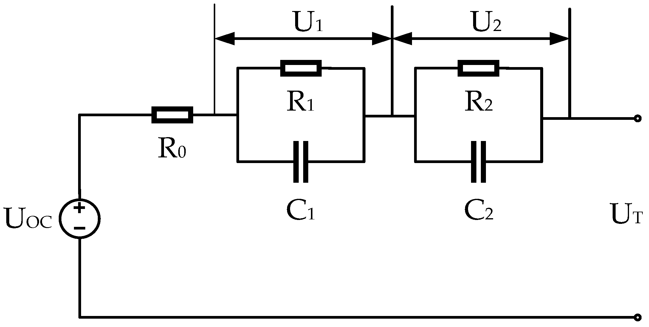
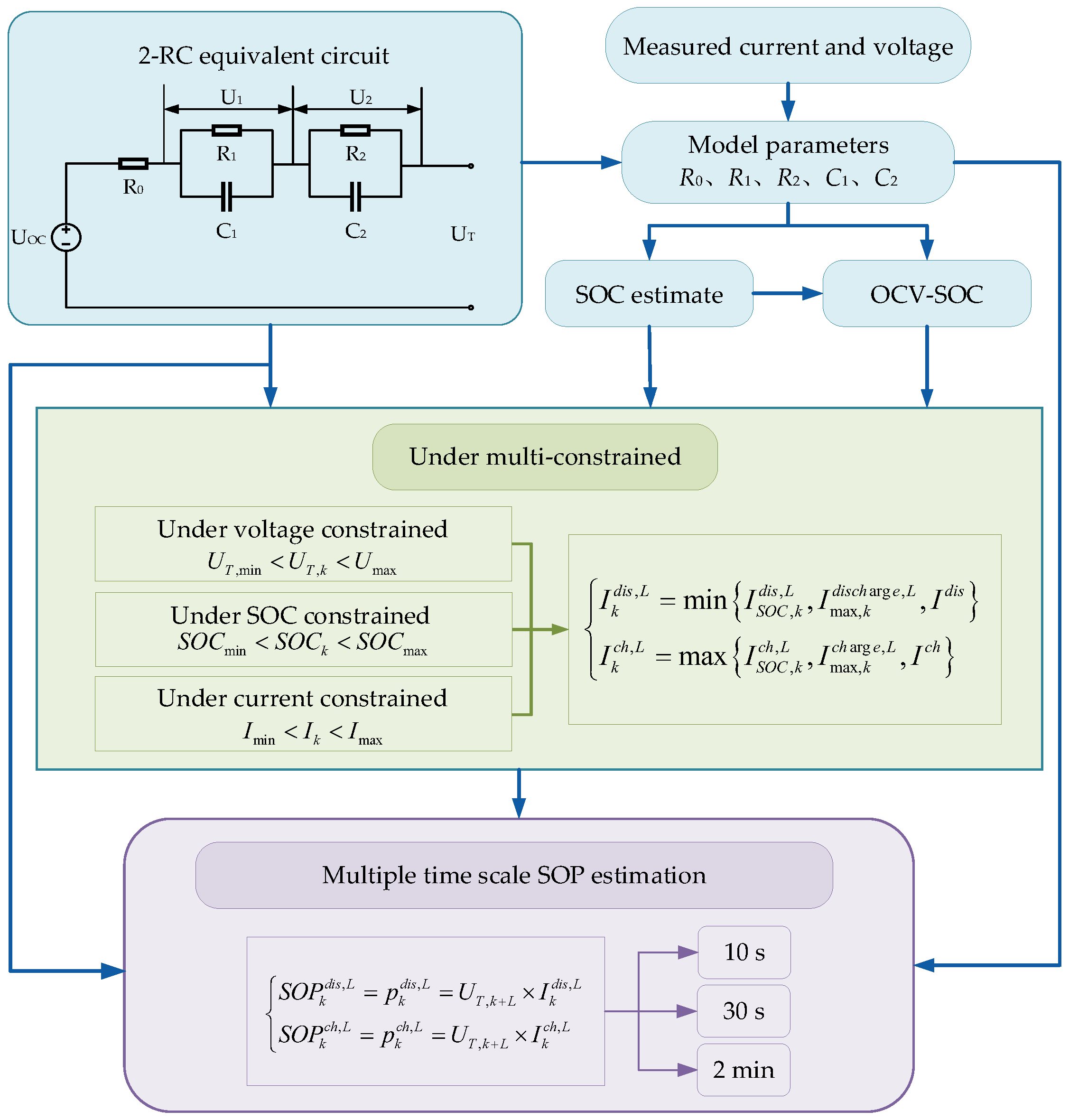
2.1. Battery Modeling

To reduce the complexity of the model and improve its accuracy, this paper adopts the second-order RC equivalent circuit model, as shown in Figure 2.

The state equation of the battery model is as follows:

$$\left[\begin{array}{c}SO{C}_k\\ U_{1,k}\\ U_{2,k}\end{array}\right]=\left[\begin{array}{ccc}1& 0& 0\\ 0& e^{\frac{-\Delta t}{R_1{C}_1}}& 0\\ 0& 0& e^{\frac{-\Delta t}{R_2{C}_2}}\end{array}\right]\left[\begin{array}{c}SO{C}_{k-1}\\ U_{1{,}_{k-1}}\\ U_{2{,}_{k-1}}\end{array}\right]+\left[\begin{array}{c}\frac{-\Delta t}{C\cdot 3600}\eta \\ \left(1-e^{\frac{-\Delta t}{R_1{C}_1}}\right)R_1\\ \left(1-e^{\frac{-\Delta t}{R_2{C}_2}}\right)R_2\end{array}\right]I_{k-1}$$

(1)

$$U_{T,k+1}=U_{OCV}\left(SO{C}_k\right)-R_0{I}_k-U_1-U_2,$$

(2)

where $U_{T,k+1},$ is the value of the terminal voltage at the moment, $U_{OCV}\left(SO{C}_k\right)$ is the open circuit voltage as a function of SOC, $R_0$ is the ohmic resistance, $R_1$ and $R_2$ are the polarization resistances, $C_1$ and $C_2$ denote the polarized capacitance, $I_{k-1}$ denotes the operating current at the $k-1$ moment, where $\eta$ is the Coulomb efficiency, and C is the battery capacity.

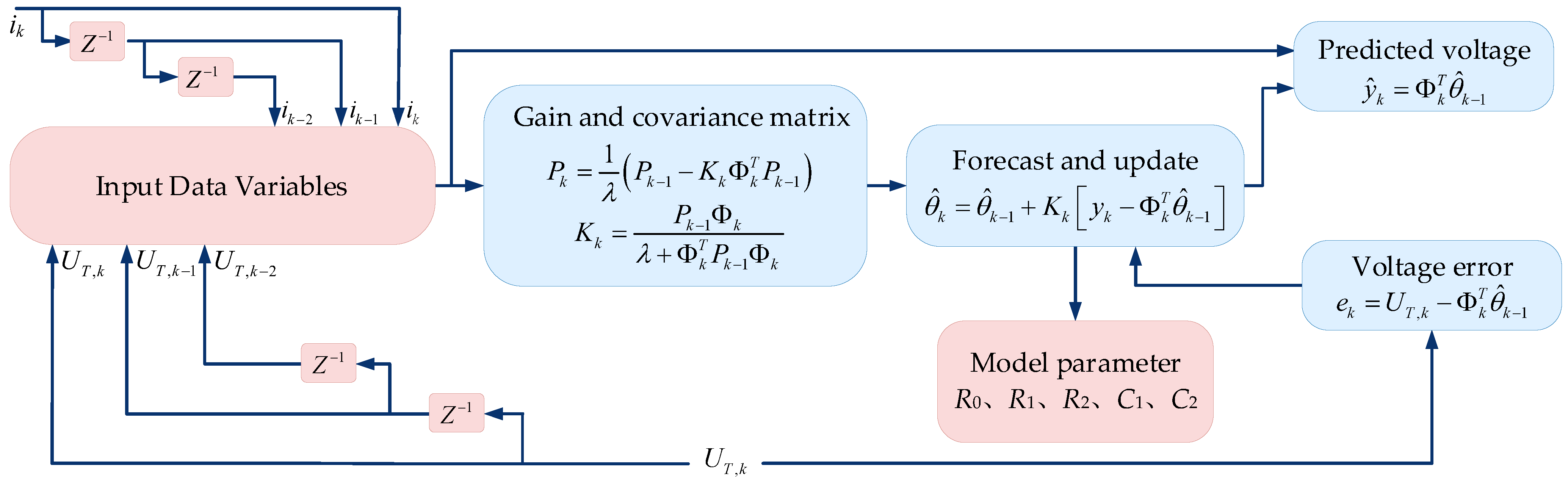
2.2. Forgetting Factor Recursive Least Squares (FFRLS)

In this paper, the FFRLS method is used to identify the model parameters online, which can not only reduce the length of computation, but also have high accuracy, prevent the algorithm from data saturation, and enhance the tracking and correction ability of the algorithm. The performance index of the FFRLS method is as follows:

$$J={{\displaystyle \sum _{k=1}^N{\lambda }^{N-k}\left[y_k-{\mathsf{\Phi }}_k^T{\widehat{\theta }}_{k-1}\right]}}^2,$$

(3)

For the performance index Equation (3), the FFRLS method equation is obtained as follows:

$${\widehat{\theta }}_k={\widehat{\theta }}_{k-1}+K_k\left[y_k-{\mathsf{\Phi }}_k^T{\widehat{\theta }}_{k-1}\right]$$

(4)

$$K_k=\frac{P_{k-1}{\mathsf{\Phi }}_k}{\lambda +{\mathsf{\Phi }}_k^T{P}_{k-1}{\mathsf{\Phi }}_k}$$

(5)

$$P_k=\frac{1}{\lambda }\left(P_{k-1}-K_k{\mathsf{\Phi }}_k^T{P}_{k-1}\right),$$

(6)

where ${\widehat{\theta }}_{k-1}$ denotes the estimated value of the parameter at the previous moment, ${\mathsf{\Phi }}_k^T{\widehat{\theta }}_{k-1}$ denotes the observed value at the current moment, $y_k$ denotes the actual observed value at the current moment, $K_k$ denotes the gain term, and the revised value of the predicted value at the current moment is the product of the expected error and the gain term, while the final estimate is the sum of the revised value of the predicted value at the current moment and the estimated value at the current moment, and $\lambda$ is the forgetting factor. In general, the forgetting factor takes a range of values $0.95<\lambda <1$, the size of $\lambda$, which affects the algorithm tracking ability. The flowchart of FFRLS identifying parameters is shown in Figure 3.

3. Joint Multi-Time Scale SOC-SOP Estimation

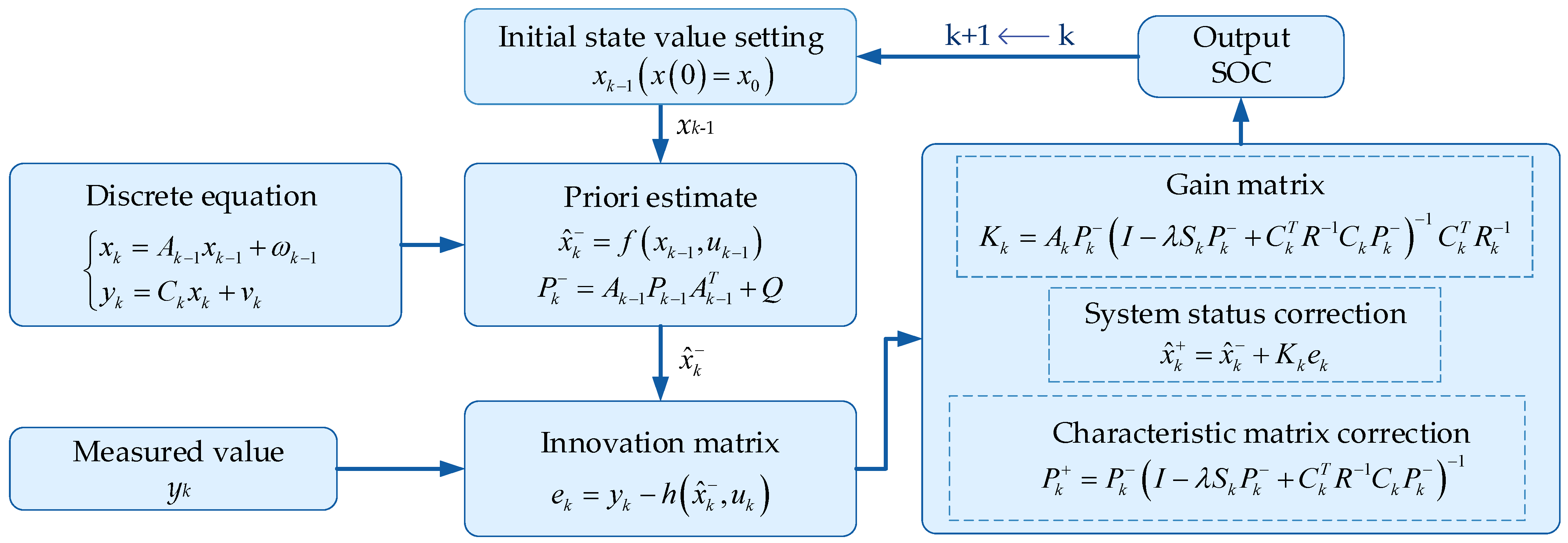
3.1. H∞ Filtering

Accurate SOC estimation is not only crucial to ensuring the charging and discharging of the lithium–ion battery of electric vehicles within the working range, but also essential for improving the life and safety of the lithium–ion battery of electric vehicles, optimizing the driving conditions, and ensuring the efficiency of energy utilization by electric vehicles. It is also an important factor affecting the accuracy of SOP estimation.

The design of the H∞ filtering algorithm is that it is not required to predict the precise statistical characteristics of noise, so as to minimize the impact of system process noise, measurement noise and uncertainty of initial state variables on the estimation accuracy, minimize the estimation error in the worst case, suppress the impact of noise on the expected output, and achieve a better anti-interference performance.

The following discrete systems are established:

$$\left\{\begin{array}{l}{x}_k=A_{k-1}{x}_{k-1}+{\omega }_{k-1}\\ y_k=C_k{x}_k+v_k\end{array}\right.,$$

(7)

where ${\omega }_{k-1}$ and $v_k$ are system process noise and measurement noise, respectively. These noises may be random, with unknown statistical characteristics or known, and the mean value of noise may be non-zero.

The design principle of the H∞ algorithm is as follows: In order to obtain the optimal estimation value at time k, the cost function is defined as $J_1$, and the objective of estimation is to find an estimation value ${\widehat{x}}_k$ of $x_k$, so as to minimize the value of cost function $J_1$. However, there are interferences in nature, and these interferences (such as ${\omega }_{k-1}$ and $v_k$) maximize the cost function $J_1$. The ultimate goal of nature is to maximize the estimation error by selecting appropriate process error ${\omega }_{k-1}$, observation error $v_k$, that is, maximize $x_k-{\widehat{x}}_k$ by ${\omega }_{k-1}$ and $v_k$. Therefore, when defining the cost function $J_1$, H∞ filtering places ${\omega }_{k-1}$, $v_k$, and the estimation error on the denominator and $x_k-{\widehat{x}}_k$ on the numerator to prevent the maximization of the estimation error caused by the increase in ${\omega }_{k-1}$ and $v_k$. The defined cost function $J_1$ is as follows:

$$J_1=\frac{{\displaystyle \sum _{K=0}^{N-1}{‖x_k-{\widehat{x}}_k‖}_{S_k}^2}}{{‖x_0-{\widehat{x}}_0‖}_{P_0^{-1}}^2+{\displaystyle \sum _{K=0}^{N-1}\left({‖{\omega }_k‖}_{Q_k^{-1}}^2+{‖v_k‖}_{R_k^{-1}}^2\right)}}.$$

(8)

In the formula, $x_0$ represents the initial value set value of the state quantity, ${\widehat{x}}_0$ represents the estimated value of the state quantity, $P_0$ represents the initial state error covariance matrix, $Q_k$ represents the noise covariance matrix of the state equation, and $R_k$ represents the covariance matrix of the measurement equation, where $S_k$ is designed according to the attention paid to the state variable.

However, it is not easy to minimize the value of cost function $J_1$ in practice. If we simply make $x_0$, ${\omega }_k$, $v_k$ infinite to make the value of cost function $J_1$ infinitesimal, which does not conform to the law, it is necessary to select and design reasonable estimation strategies to minimize the cost function. Since direct minimization is difficult to achieve, we often choose a performance boundary $\lambda$ to meet the following requirements:

$$J_1<\frac{1}{\lambda },$$

(9)

Reorganizing Formula (8), we can obtain that the cost function $J_2$ based on the performance boundary is

$$J_2=-\frac{1}{\lambda }{‖x_0-{\widehat{x}}_0‖}_{P_0^{-1}}^2+{\displaystyle \sum _{k=0}^{N-1}\left({‖x_0-{\widehat{x}}_0‖}_{S_k}^2-\frac{1}{\lambda }\left({‖{\omega }_k‖}_{Q_k^{-1}}^2+{‖v_k‖}_{R_k^{-1}}^2\right)\right)}<0.$$

(10)

By rearranging the formula, the objective is as follows. When $x_0$, ${\omega }_k$, and $v_k$ make $J_2$ maximum, the appropriate ${\widehat{x}}_k$ that makes $J_2$ minimum is chosen. The recurrence relation that makes the cost function $J_1$ smaller than $1/\lambda$ can be obtained after calculation as follows:

$$\left\{\begin{array}{l}{K}_k=P_k{\left(I-\lambda S_k{P}_k+C_k^T{R}_k^{-1}{C}_k{P}_k\right)}^{-1}{C}_k^T{R}_k^{-1}\\ {\widehat{x}}_{k+1}=A_k{\widehat{x}}_k+A_k{K}_k\left(y_k-C_k{\widehat{x}}_k\right)\\ P_{k+1}=A_k{P}_k{\left(I-\lambda S_k{P}_k+C_k^T{R}_k^{-1}{C}_k{P}_k\right)}^{-1}{A}_k^T+Q_k\end{array}\right.,$$

(11)

where $K_k$ is the gain matrix, $P_k$ is the selected symmetric positive definite array, and $P_0$ is the matrix obtained based on the above recurrence relation.

To better distinguish the estimation results obtained before and after the update, ${\widehat{x}}_k^{-}$ is used to denote the value of ${\widehat{x}}_k$ after the time update, $P_k^{-}$ is used to denote the value of $P_k$ after the time update, ${\widehat{x}}_k^{+}$ is used to denote the value of ${\widehat{x}}_k$ after the measurement update, and $P_k^{+}$ is used to denote the value of $P_k$ after the measurement update. The flowchart of this algorithm is shown in Figure 4.

3.2. Multi-Time Scale SOP Estimation

The accurate estimation of SOP of the lithium–ion battery can not only ensure the optimal power distribution, but also avoid overcharge and overdischarge, which extends the service life of the lithium–ion battery. The sustained peak SOP is mainly limited by three conditions: the current terminal voltage, the current SOC size, and the design limit of the battery itself. The actual running state of the electric vehicle works continuously with the time peak current of a few seconds or dozens of seconds, and the continuous peak power state has more characterization significance than the instantaneous peak power state (the peak power capacity at the next moment, which means that ΔT is 1 s). In this paper, the SOC estimation strategy is adopted to establish a joint estimation algorithm of multi-time scale SOP.

In this paper, SOP is defined as the continuous peak power level that the battery can reach in the next specified time range:

$$\left\{\begin{array}{l}SO{P}^{dis}=p^{dis}=U_T\times I^{dis}\\ SO{P}^{ch}=p^{ch}=U_T\times I^{ch}\end{array}\right.,$$

(12)

where $SO{P}^{dis}$ and $SO{P}^{ch}$ are discharge SOP and charge SOP, respectively, $p^{dis}$ and $p^{ch}$ are discharge power and charge power, respectively, $U_T$ is terminal voltage, $I^{dis}$ and $I^{ch}$ are the peak discharge current and peak charge current that the battery can maintain in the next time range, respectively.

$\Delta t$ is the sampling time. It is assumed that the peak current from k sampling time to k + L sampling time is constant, which means that $I_{k+1}=I_{k+2}=I_{k+L}$. Then, the polarization voltage at k + L sampling time can be expressed as follows:

$$\left\{\begin{array}{l}{U}_{1,k+L}=U_{1,k}{e}^{-\frac{L\times \Delta t}{{\tau }_1}}+\left(1-e^{-\frac{L\times \Delta t}{{\tau }_1}}\right)R_1{I}_{k+L}\\ U_{2,k+L}=U_{2,k}{e}^{-\frac{L\times \Delta t}{{\tau }_2}}+\left(1-e^{-\frac{L\times \Delta t}{{\tau }_2}}\right)R_2{I}_{k+L}\end{array}\right..$$

(13)

By using Taylor formula to expand $U_{OC}\left(SO{C}_{k+L}\right)$ at k sampling time, and ignoring multiple higher-order terms, we can obtain

$$U_{OC}\left(SO{C}_{k+L}\right)=U_{OC}\left(SO{C}_k\right)-I_{T,k+L}\frac{L\times \Delta t}{Q_n}\frac{\partial U_{OC}\left(SO{C}_k\right)}{\partial SO{C}_k}.$$

(14)

Then, the terminal voltage $U_{T,k+L}$ of the lithium–ion battery after the action of a continuous current for time $L\times \Delta t$ can be expressed as follows:

$$\begin{array}{l}{U}_{T,k+L}=U_{OC}\left(SO{C}_k\right)-U_{1,k}{e}^{-\frac{L\times \Delta t}{{\tau }_1}}-U_{2,k}{e}^{-\frac{L\times \Delta t}{{\tau }_2}}\\ -I_{T,k+L}\left[\frac{L\times \Delta t}{Q_n}\frac{\partial U_{OC}\left(SO{C}_k\right)}{\partial SO{C}_k}+R_0+\left(1-e^{-\frac{L\times \Delta t}{{\tau }_1}}\right)R_1+\left(1-e^{-\frac{L\times \Delta t}{{\tau }_2}}\right)R_2\right]\end{array}.$$

(15)

Then, the current at the moment k + L can be expressed as follows:

$$I_{T,k+L}=\frac{U_{OC}\left(SO{C}_k\right)-U_{1,k}{e}^{-\frac{L\times \Delta t}{{\tau }_1}}-U_{2,k}{e}^{-\frac{L\times \Delta t}{{\tau }_2}}-U_{T,k+L}}{\frac{L\times \Delta t}{Q_n}\frac{\partial U_{OC}\left(SO{C}_k\right)}{\partial SO{C}_k}+R_0+\left(1-e^{-\frac{L\times \Delta t}{{\tau }_1}}\right)R_1+\left(1-e^{-\frac{L\times \Delta t}{{\tau }_2}}\right)R_2}.$$

(16)

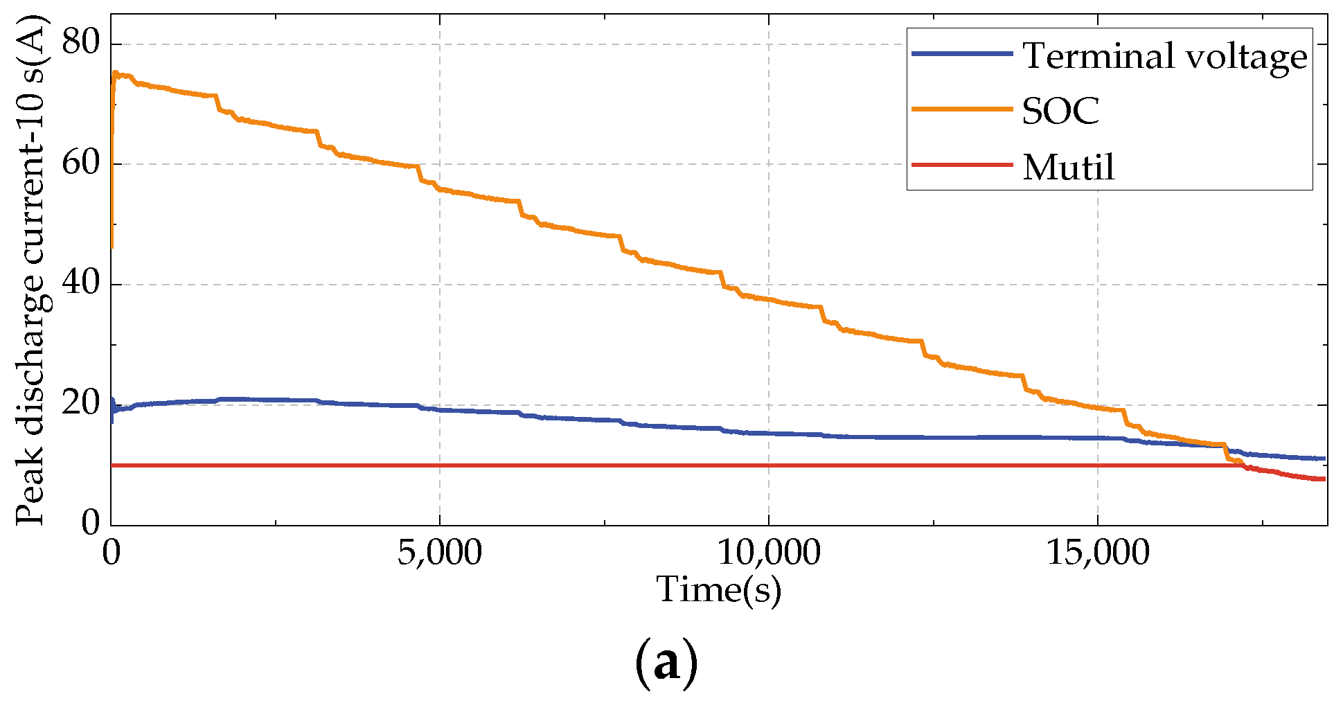
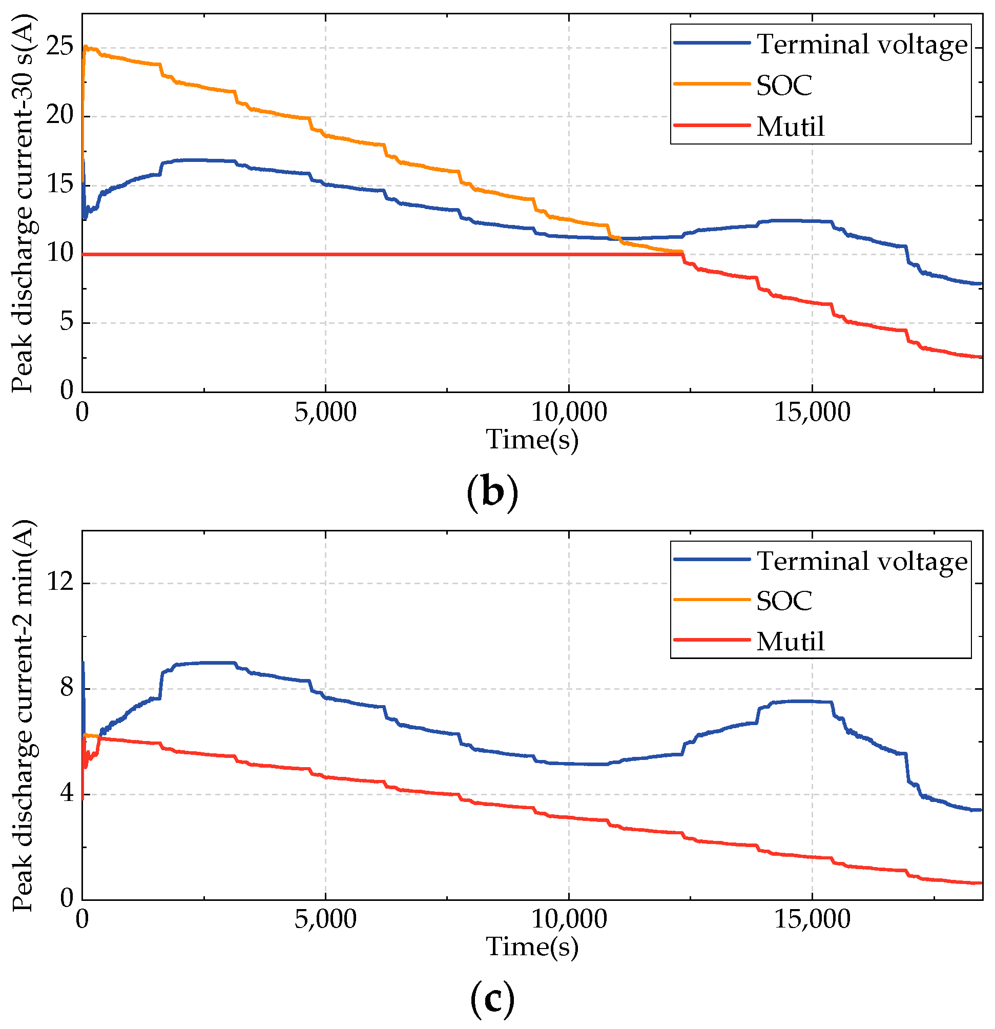
3.2.1. Continuous Peak Current Based on Voltage Constraints

For the lithium–ion batteries in actual operation, it is necessary to consider the existence of end voltage design limits (charge or discharge cut-off voltage). That is to say, the operating voltage at any moment needs to meet the condition that $U_{T,\min }<U_{T,k}<U_{\max }$. Therefore, the charge and discharge sustained peak currents at end voltage limits (maximum 4.2 V, minimum 2.75 V) are expressed as follows:

$$\left\{\begin{array}{l}{I}_{\max ,k}^{\mathrm{discharge},L}=\frac{U_{OC}\left(SO{C}_k\right)-U_{1,k}{e}^{-\frac{L\times \Delta t}{{\tau }_1}}-U_{2,k}{e}^{-\frac{L\times \Delta t}{{\tau }_2}}-U_{T,\min }}{\frac{L\times \Delta t}{Q_n}\frac{\partial U_{OC}\left(SO{C}_k\right)}{\partial SO{C}_k}+R_0+\left(1-e^{-\frac{L\times \Delta t}{{\tau }_1}}\right)R_1+\left(1-e^{-\frac{L\times \Delta t}{{\tau }_2}}\right)R_2}\\ I_{\max ,k}^{\mathrm{charge},L}=\frac{U_{OC}\left(SO{C}_k\right)-U_{1,k}{e}^{-\frac{L\times \Delta t}{{\tau }_1}}-U_{2,k}{e}^{-\frac{L\times \Delta t}{{\tau }_2}}-U_{T,\max }}{\frac{L\times \Delta t}{Q_n}\frac{\partial U_{OC}\left(SO{C}_k\right)}{\partial SO{C}_k}+R_0+\left(1-e^{-\frac{L\times \Delta t}{{\tau }_1}}\right)R_1+\left(1-e^{-\frac{L\times \Delta t}{{\tau }_2}}\right)R_2}\end{array}\right.,$$

(17)

where $I_{\max ,k}^{\mathrm{discharge},L}$ and $I_{\max ,k}^{\mathrm{charge},L},$ are the estimates of the peak continuous discharge current and the peak continuous charge current at the moment of k sampling based on the voltage limitation condition at the model’s end, respectively.

3.2.2. Continuous Peak Current Based on SOC Constraints

In order to ensure the safe operation of the lithium–ion battery pack for electric vehicles, the SOC of the lithium–ion battery at any moment is required to meet a certain restrictions, that is, $SO{C}_{\min }<SO{C}_k<SO{C}_{\max }$ (where the maximum SOC is 100% and the minimum is 0%). Then, under the limit of SOC at the current moment, the continuous peak discharge current and continuous peak charge current for the future time period $L\times \Delta t$ can be expressed, respectively, as follows:

$$\left\{\begin{array}{l}{I}_{SOC,k}^{dis,L}=\frac{SO{C}_k-SO{C}_{\min }}{\frac{\Delta t}{Q_n}}\\ I_{SOC,k}^{ch,L}=\frac{SO{C}_k-SO{C}_{\max }}{\frac{\Delta t}{Q_n}}\end{array}\right.,$$

(18)

where $SO{C}_k$ is the SOC value at the moment k, $I_{SOC,k}^{dis,L}$ denotes the maximum discharge current in the time period $L\times \Delta t$ under the current SOC conditions, and $I_{SOC,k}^{ch,L}$ denotes the maximum charge current in the time period $L\times \Delta t$ under the current SOC conditions.

3.2.3. Continuous Peak Charge/Discharge Current under Multiple Constraints

By combining the above two constraints and considering the design limits of the Li–ion battery itself (peak discharge current $I^{dis}$ and peak charge current $I^{ch}$), the sustained peak charge and discharge current with multiple constraints can be obtained:

$$\left\{\begin{array}{l}{I}_k^{dis,L}=\min \left\{I_{SOC,k}^{dis,L},I_{\max ,k}^{\mathrm{discharge},L},I^{dis}\right\}\\ I_k^{ch,L}=\max \left\{I_{SOC,k}^{ch,L},I_{\max ,k}^{\mathrm{charge},L},I^{ch}\right\}\end{array}\right.,$$

(19)

where $I_k^{dis,L}$ indicates the maximum discharge current in the next $L\times \Delta t$ time period, and $I_k^{ch,L}$ indicates the maximum charge current in the next $L\times \Delta t$ time period.

Based on Formula (15), the SOP of lithium–ion battery in the time period $L\times \Delta t$ is expressed as follows:

$$\left\{\begin{array}{l}SO{P}_k^{dis,L}=p_k^{dis,L}=U_{T,k+L}\times I_k^{dis,L}\\ SO{P}_k^{ch,L}=p_k^{ch,L}=U_{T,k+L}\times I_k^{ch,L}\end{array}\right..$$

(20)

3.2.4. Algorithm Flow

Model based peak power estimation is currently the mainstream estimation method. However, using SOC based methods alone or considering only single parameter constraints can often cause safety issues such as excessive instantaneous peak current. Combining the previous derivation process, SOP estimation with multiple constraints is performed. Firstly, a second-order RC equivalent circuit model is established, and the measured voltage and current are used as input for parameter identification. Then, combined with the results of SOC estimation using the H∞ algorithm, the battery design limits, and the current terminal voltage constraints, the continuous peak SOP is jointly estimated under multiple constraints, and the accuracy of SOP estimation under different time scales is verified. The algorithm flow is shown in Figure 5.

4. Validations and Discussion

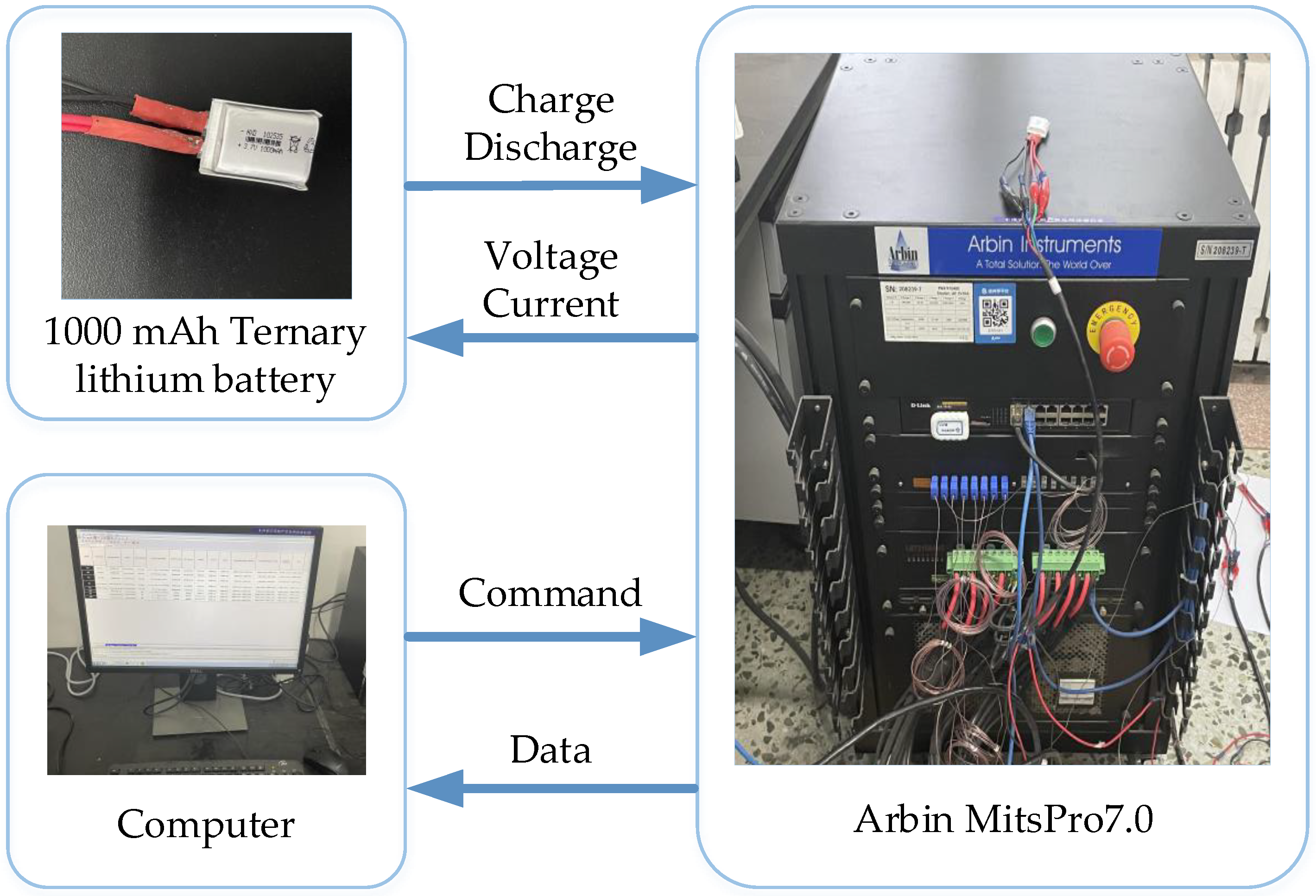
4.1. Experimental Setup and Test Procedure

In this paper, a ternary lithium–ion battery with a rated capacity of 1000 mAh is used as the experimental object. As shown in Figure 6, the test platform consists of the host computer, the battery under test, and the battery test system of ArbinMitsPro7.0 to conduct the following experiments.

• Battery capacity test

  (1)

  Charge the battery with a current from 0.5 C to 4.2 V, and then change it to a constant voltage of 4.2 V to charge the battery. When the charging current drops to 50 mA, stop charging, and the battery is considered to be fully charged;

  (2)

  Let stand for 2 h;

  (3)

  Discharge at a constant current of 0.2 C until the terminal voltage is less than 2.75 V, and integrate the discharge current with time, that is, use the ampere-hour integration method to obtain the current discharge capacity;

  (4)

  Repeat steps (1) to (3) three times. If the error of the capacity obtained for three times is less than 2%, take the average of the three discharge capacities as the maximum usable capacity, otherwise repeat steps (1) to (3) until the requirements are met.

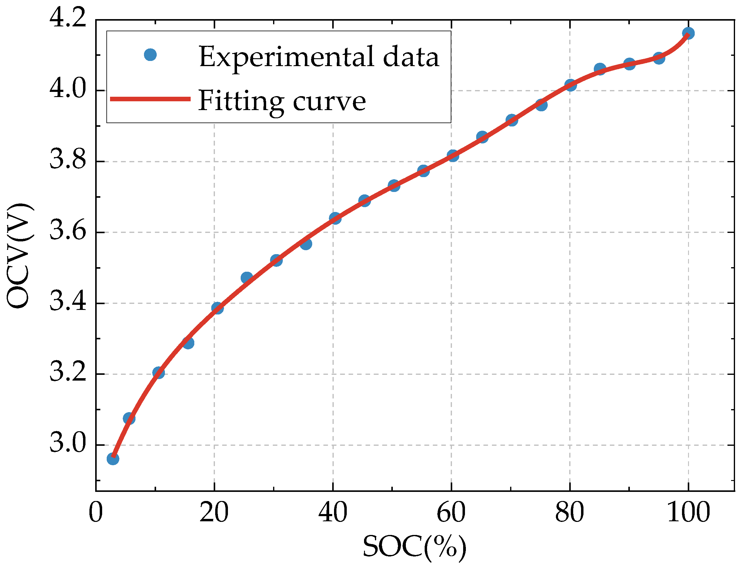
• Open-circuit voltage test

  (1)

  Charge the battery to 4.2 V with a current of 0.5 C, and then convert it to a constant voltage of 4.2 V to charge the battery pack. When the charging current drops to 50 mA, stop charging, and then the battery is considered to be fully charged;

  (2)

  After standing for 2 h, the measured terminal voltage is OCV when fully charged (i.e., SOC = 100%);

  (3)

  Discharge at 1C constant current for 3 min, and then let it stand for 2 h. The terminal voltage after standing for 2 h is the OCV under the current SOC state;

  (4)

  Repeat the third step until the terminal voltage of the tested object is less than 2.75 V and stop discharging, and collect the experimental data.

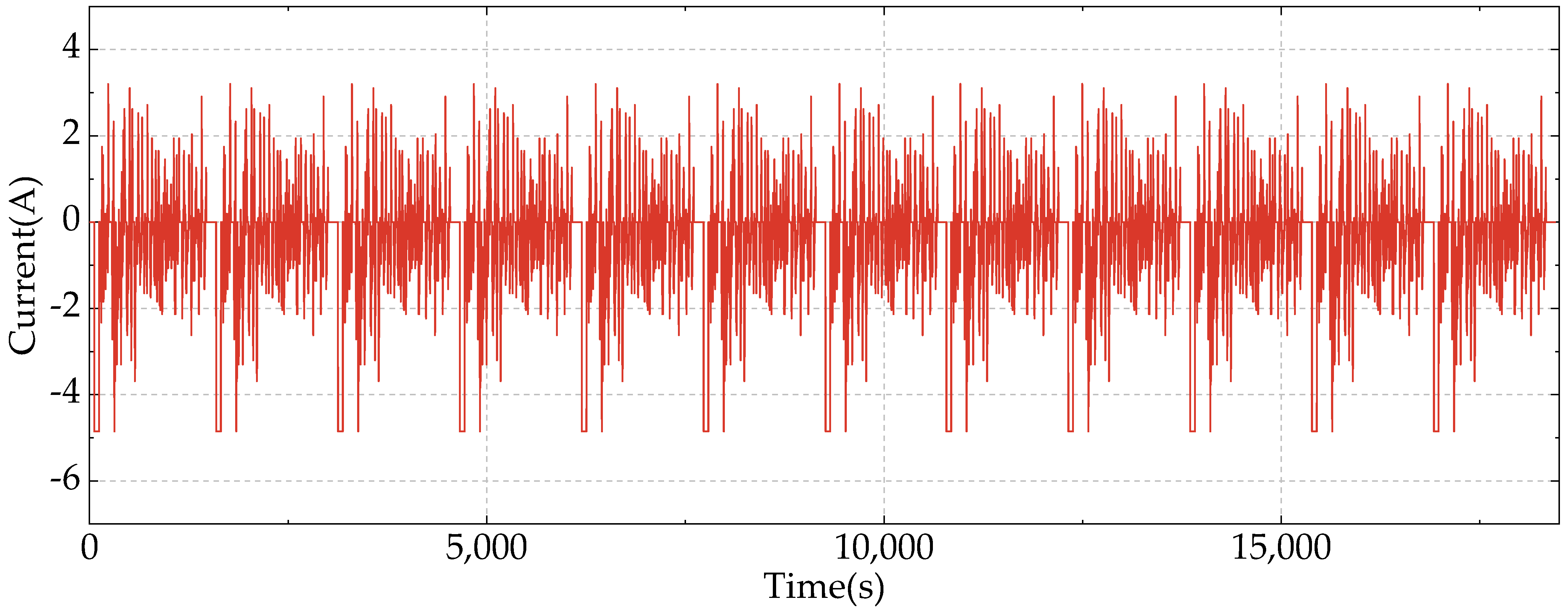
• UDDS working condition test

In order to provide data support for the accuracy of the proposed state estimation algorithm under actual dynamic conditions, the robustness of the algorithm is verified through the UDDS condition test to simulate the working condition of the battery when it is used on the actual vehicle.

(1)

Charge the battery with a current of 0.5 C to 4.2 V, and then change it to a constant voltage of 4.2 V to charge the battery. When the charging current drops to 50 mA, stop charging, and the battery is considered to be fully charged;

(2)

Let stand for 2 h;

(3)

Input the UDDS working condition excitation current (as shown in Figure 7) into the battery test system to conduct the cyclic working condition test until the terminal voltage of the tested object is less than 2.75 V and stop discharging, and collect the experimental data.

In order to verify the accuracy of estimation by the algorithm proposed in this paper, three mathematical indicators, namely, relative error (RE), mean absolute relative error (MARE), and root mean square error (RMSE), are used to evaluate the joint estimation performance of SOC–SOP.

The definitions are given out as follows:

$$RE=\frac{y^{\ast }-y}{y}$$

(21)

$$MARE=\frac{1}{N}{\displaystyle \sum _1^N\left|\frac{y^{\ast }-y}{y}\right|}$$

(22)

$$RMSE=\sqrt{\frac{1}{N}{\displaystyle \sum _1^N{\left(y^{\ast }-y\right)}^2}},$$

(23)

where $y^{\ast }$ is the estimated value, $y$ is the reference value, and $N$ is the number of samples.

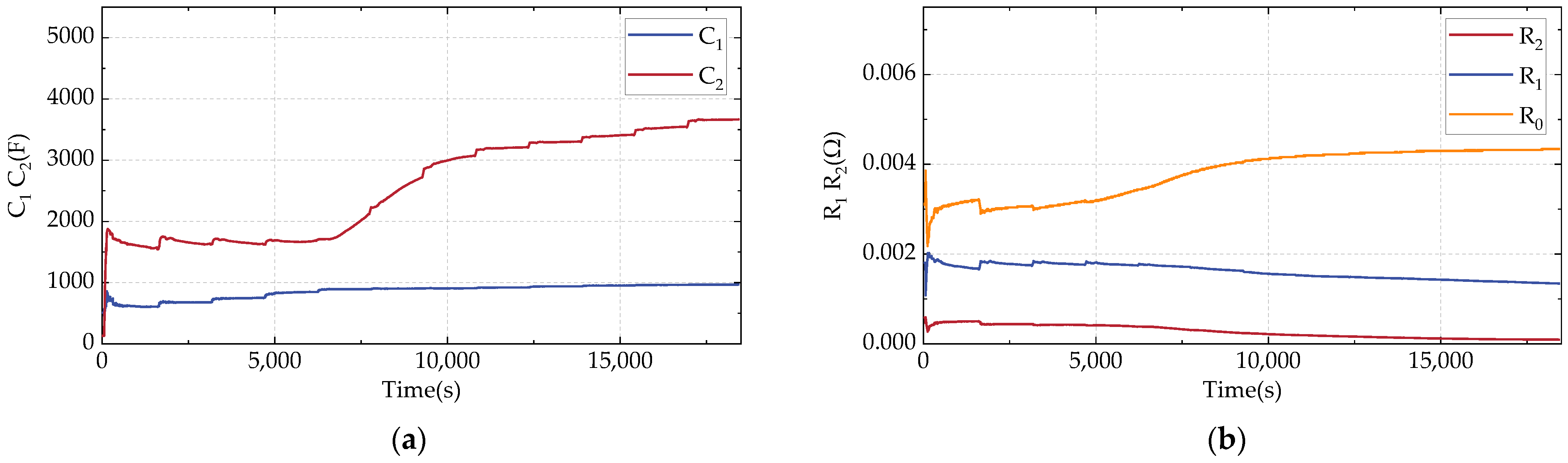
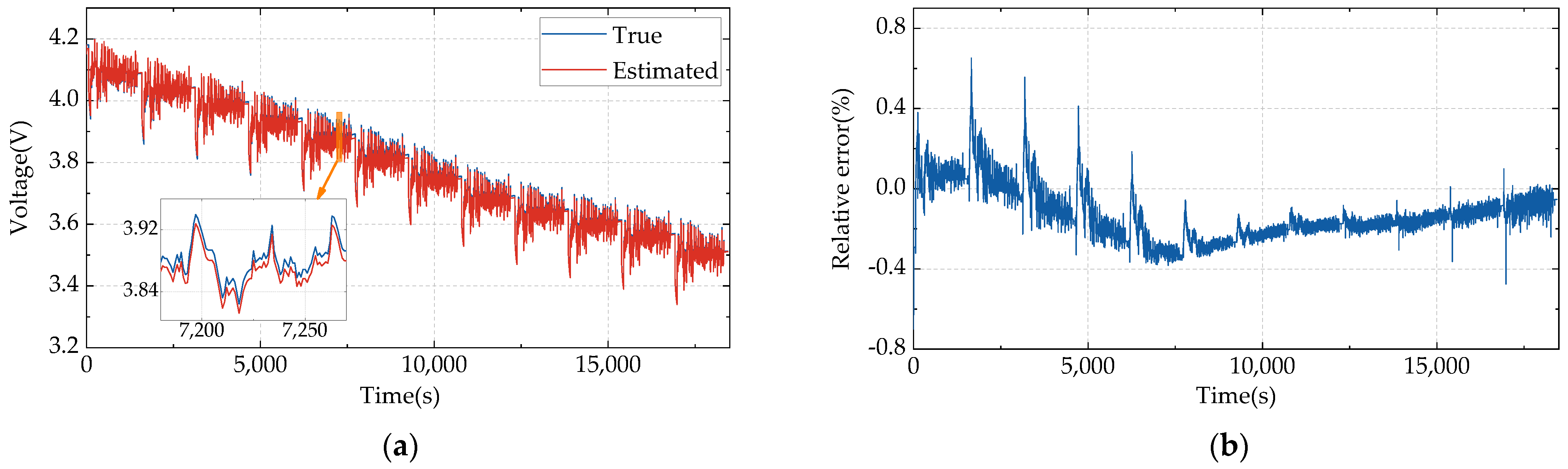
4.2. Validation of FFRLS Parameter Identification Results

The open-circuit voltage (OCV)–SOC relationship curve of the battery is obtained by using the constant-current discharge gap method. An eighth-order polynomial fit is performed in MATLAB to obtain the expression of the battery open-circuit voltage as a function of SOC below:

$$U_{OCV}=k_{1}SO{C}^8+k_{2}SO{C}^7+k_{3}SO{C}^6+k_{4}SO{C}^5+k_{5}SO{C}^4+k_{6}SO{C}^3+k_{7}SO{C}^2+k_{8}SO{C}^1+k_9.$$

(24)

The OCV–SOC fitting curve was obtained, as shown in Figure 8.

Based on the mathematical form of the second-order RC equivalent circuit model derived above, online parameter identification is performed with the data of UDDS operating conditions as input. The five parameters (R₀, R₁, R₂, C₁, C₂) as identified by the FFRLS online are shown in Figure 9.

As for C₁ and C₂ in the previous stage of identification, the circuit model parameters change more significantly due to the differences in the selection of the initial values of the model parameters and the large deviations caused by their initial values. Moreover, the values of each parameter gradually stabilize as the identification process continues. Therefore, as can be seen from Figure 9, even if the given initial values are inaccurate, the FFRLS algorithm can still correct each parameter in time, so that the parameters converge rapidly to approach the true value and remain stable. The five parameters are iteratively updated in real time according to the UDDS operating data, so that the battery model can be transformed into a time-varying system. Thus, the self-adaptation of the battery model parameters is achieved and the estimation accuracy of the battery state is improved.

In order to evaluate the validity and accuracy of the circuit model selected in this paper, a comparison is performed between the end voltage estimated by the FFRLS algorithm and the actual measured end voltage at the end under UDDS operating conditions, as shown in Figure 10. Figure 10a shows the comparison of end voltage estimation, and Figure 10b shows the end voltage estimation error. From these two figures, it can be seen that the end voltage trend estimated by FFRLS is similar to the reference value with a small error. In the place where the larger error occurs, there are more frequent charging and discharging transitions under the operating conditions, and the time that this process lasts is too short for the end voltage to be measured accurately in time. As a result, the error becomes larger. According to the whole estimation cycle, the two curves basically overlap, the discriminated voltage RE is within ±0.8%, and MARE is only 0.58%, which indicates the high stability and high tracking accuracy of the FFRLS algorithm for parameter discrimination.

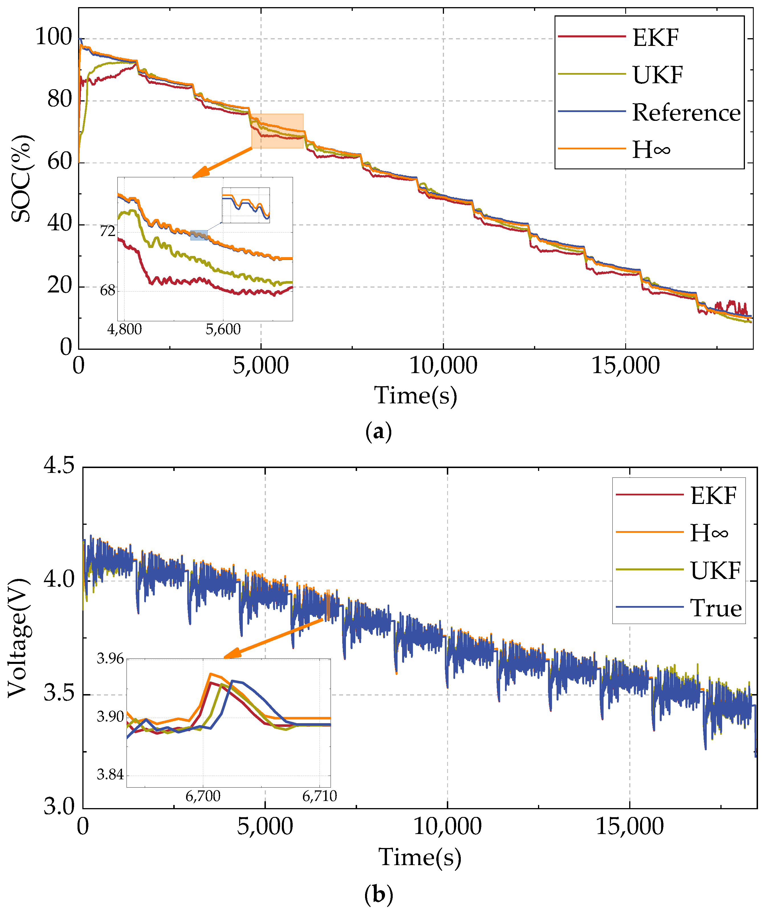
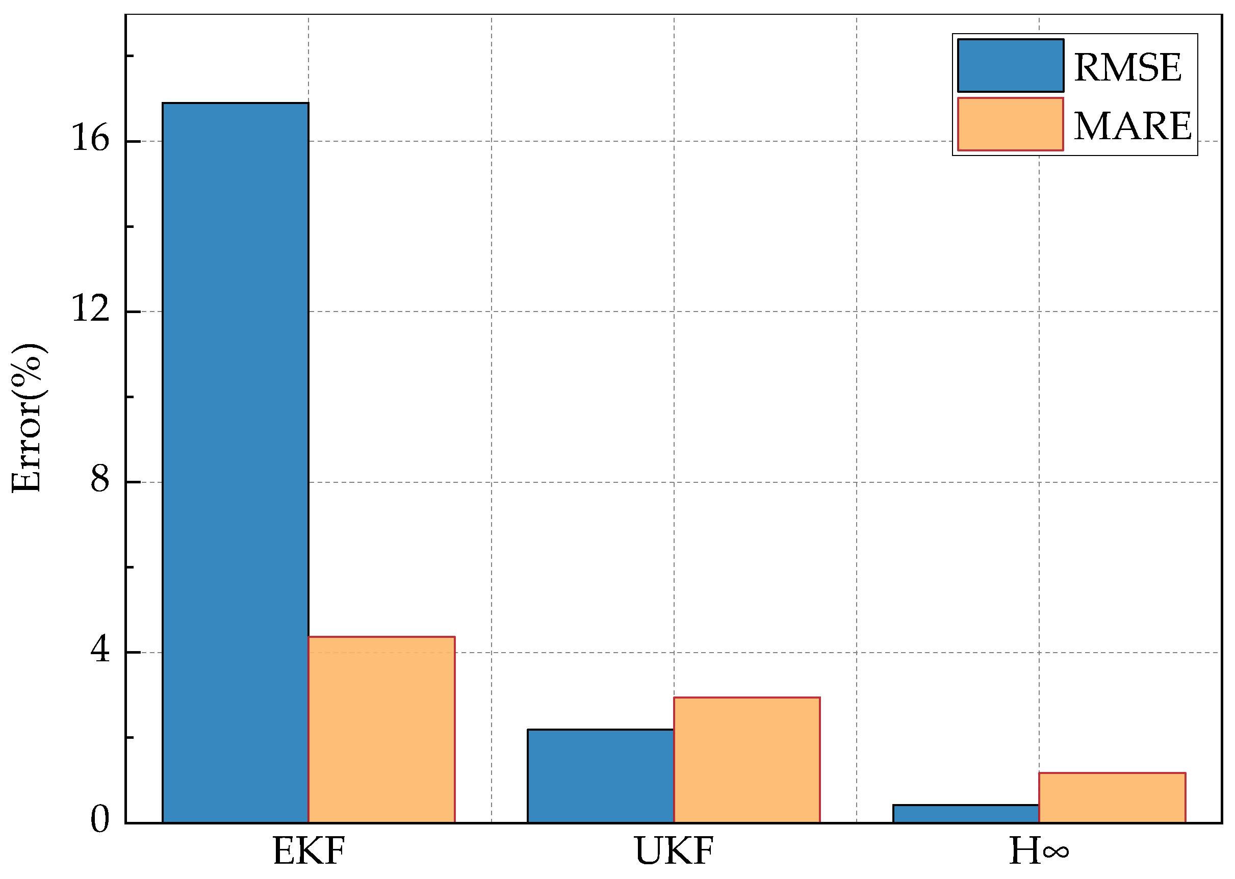
4.3. Verification of SOC Estimation

Figure 11 shows the results of SOC estimation by different methods and the corresponding terminal voltage errors under UDDS conditions. In order to evaluate the convergence and performance of the proposed method, a large initial SOC error is set in this paper. Although the initial value is uncertain in the initial stage of estimation, the H∞ algorithm can still track the SOC reference value in a very short time. Under the UDDS working condition, the current changes dramatically. In this case, the noise of the battery model is very large, the characteristics of white noise are not shown any more, and the parameters of the battery model change significantly as well due to the drastic change in the current. It can be clearly seen from the figure that the H∞ algorithm outperforms the EKF algorithm and the UKF algorithm in tracking the change of the SOC reference value. Figure 12 shows the SOC estimation error. The MARE of H∞ algorithm for estimating SOC is less than 1.5%, and the RMSE is less than 0.5%. That is to say, the proposed method of SOC estimation through the H∞ algorithm has absolute advantages.

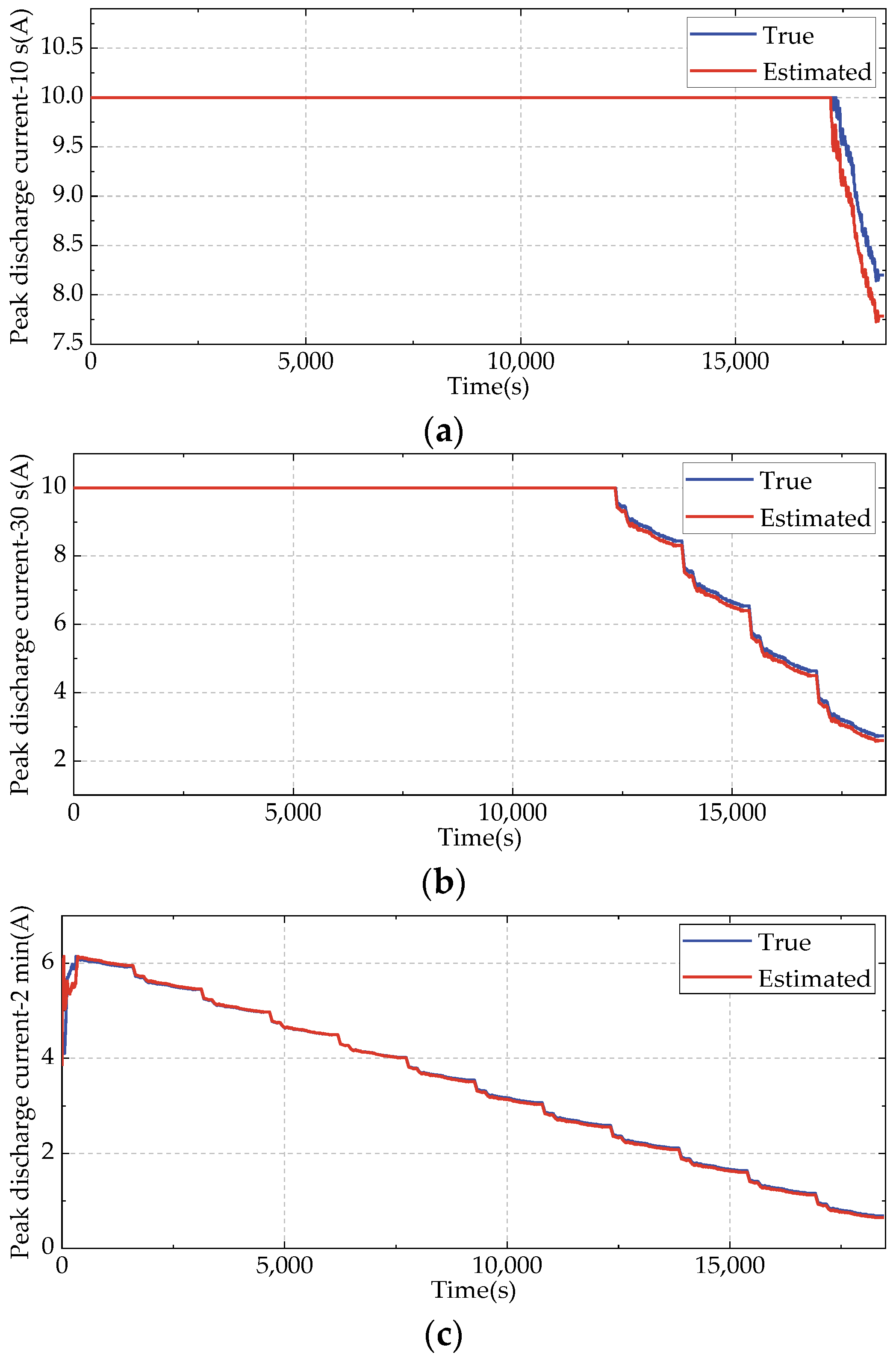
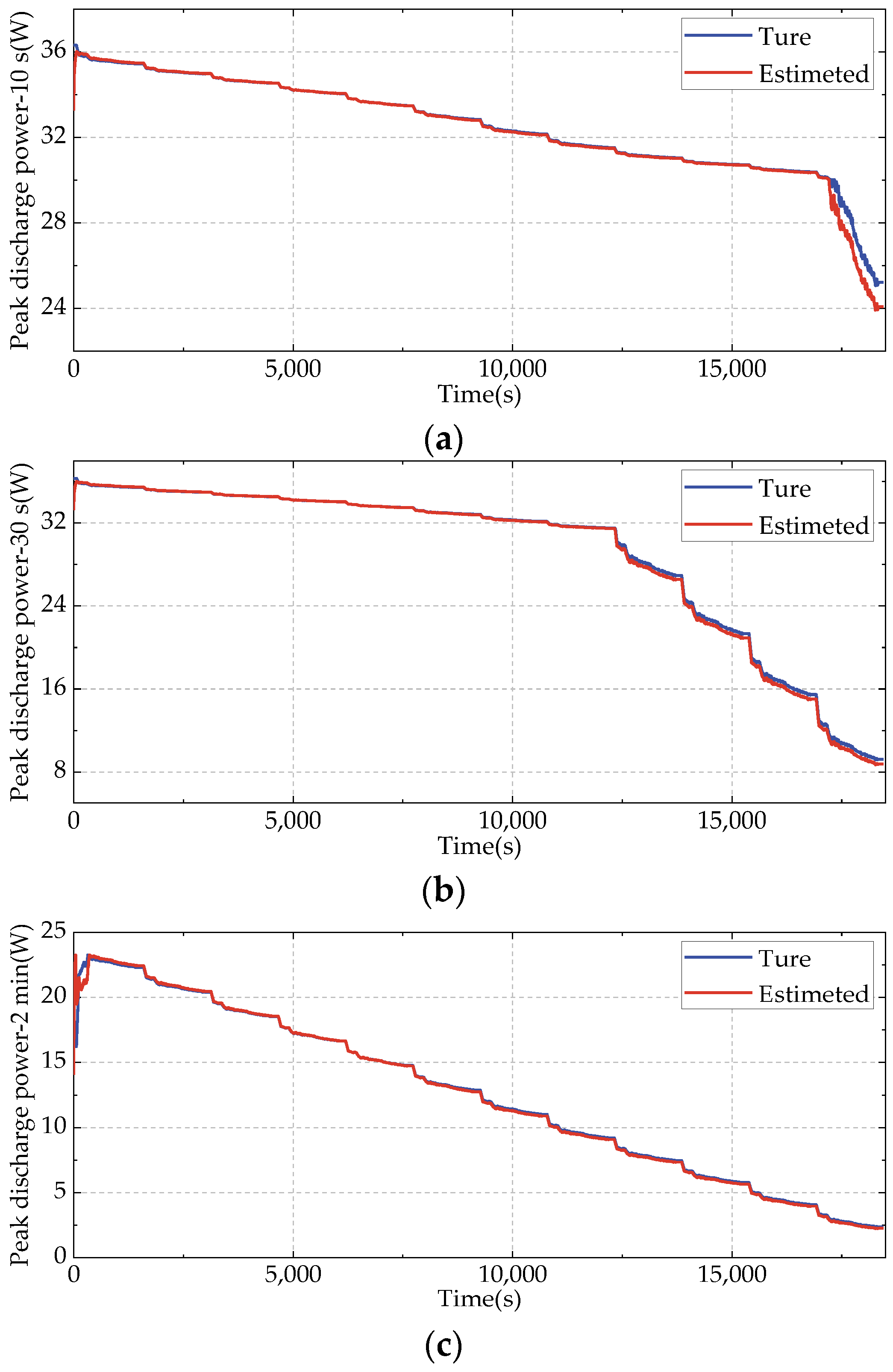
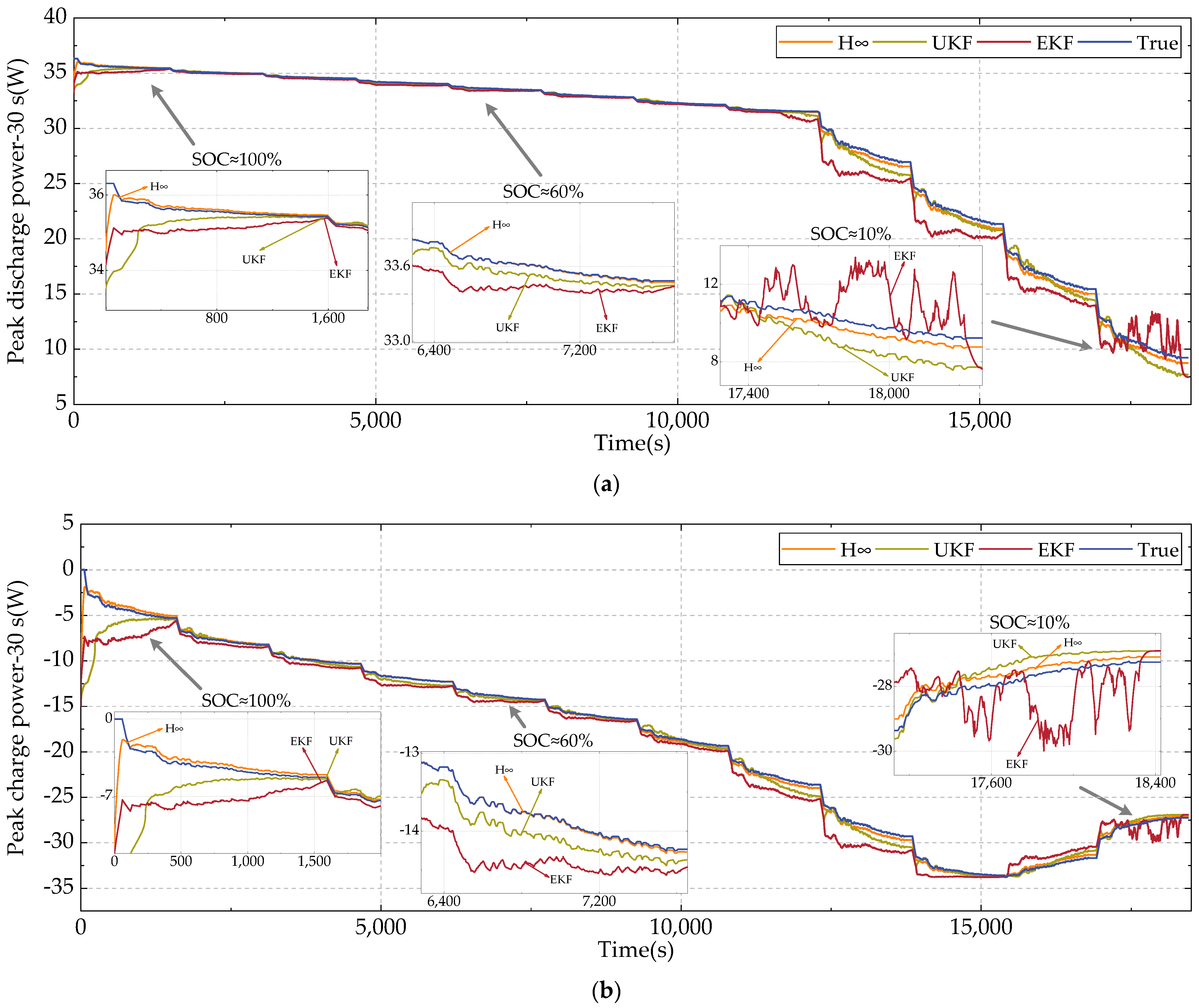
4.4. Validation Results of Online SOP Estimation

In the process of estimating the battery SOP, the main constraints on the sustained peak current include the current terminal voltage, the current SOC value, and the design limit of the battery itself. Among them, the current terminal voltage is obtained from the current SOC value combined with the OCV–SOC function relationship through the battery state equation. Therefore, in the process of SOP estimation of the Li–ion battery, the accuracy of SOP estimation is largely determined by the accuracy of SOC estimation. Based on this, the joint SOC–SOP estimation method is established in this paper, and the estimation effect of the joint estimation algorithm is verified under the dynamic working condition of UDDS.

4.4.1. Discharge SOP Estimation

Figure 13 and Figure 14 show the results of sustained peak discharge current estimation under different constraints for a duration of 10 s, 30 s, and 2 min. The sustained peak discharge current as estimated by the SOC or under the terminal voltage constraint alone is too large, which can lead to the over-discharge of the lithium–ion battery and seriously affect the battery performance and service life. The sustained peak discharge current is mainly determined by the maximum discharge current of the lithium–ion battery itself, and this phase is shortened as the discharge time increases. This is due to the fact that the longer the sustained discharge time, the easier it is to reach the set cut-off condition (end-voltage discharge cut-off condition, 2.75 V) at the same discharge current. Then, it shifts to the current SOC constraint, which is due to the fact that the peak current estimation condition based on the SOC value can reduce the current of discharge when the actual SOC value of the Li–ion battery is too low or even close to the SOC limiting condition, thus avoiding the over-discharge to the lithium–ion battery.

Figure 15 and Figure 16 show the sustained peak discharge power curves and the corresponding error results for 10 s, 30 s, and 2 min of sustained discharge. In the initial stage of estimation, the sustained peak discharge power error is large. This is because there is an error between the initial estimate of the H∞ algorithm and the true value, and as the difference in the estimated end voltages increases, there is an increase in the error of sustained peak discharge power. Therefore, increasing the convergence speed of the SOC estimation algorithm is conducive to reducing the sustained peak discharge power estimation error. In addition, the longer the duration of continuous discharge, the lower the continuous peak discharge power at the same moment. This is because the sustained peak discharge power decreases when the current of sustained discharge decreases with the extension of discharge time under multiple constraints. According to the results listed in

Table 1. Estimation errors of sustained peak charging power for different time scales.

Time Scale	RMSE (W)	MARE (%)	Title 1	Title 2	Title 3
10 s	0.4298	0.25	entry 1	data	data
30 s	0.7652	0.83	entry 2	data	data
2 min	1.3047	1.21

, the peak discharge power MARE is less than 1.5% and the RMSE is less than 1.5 W at different sustained discharge times.

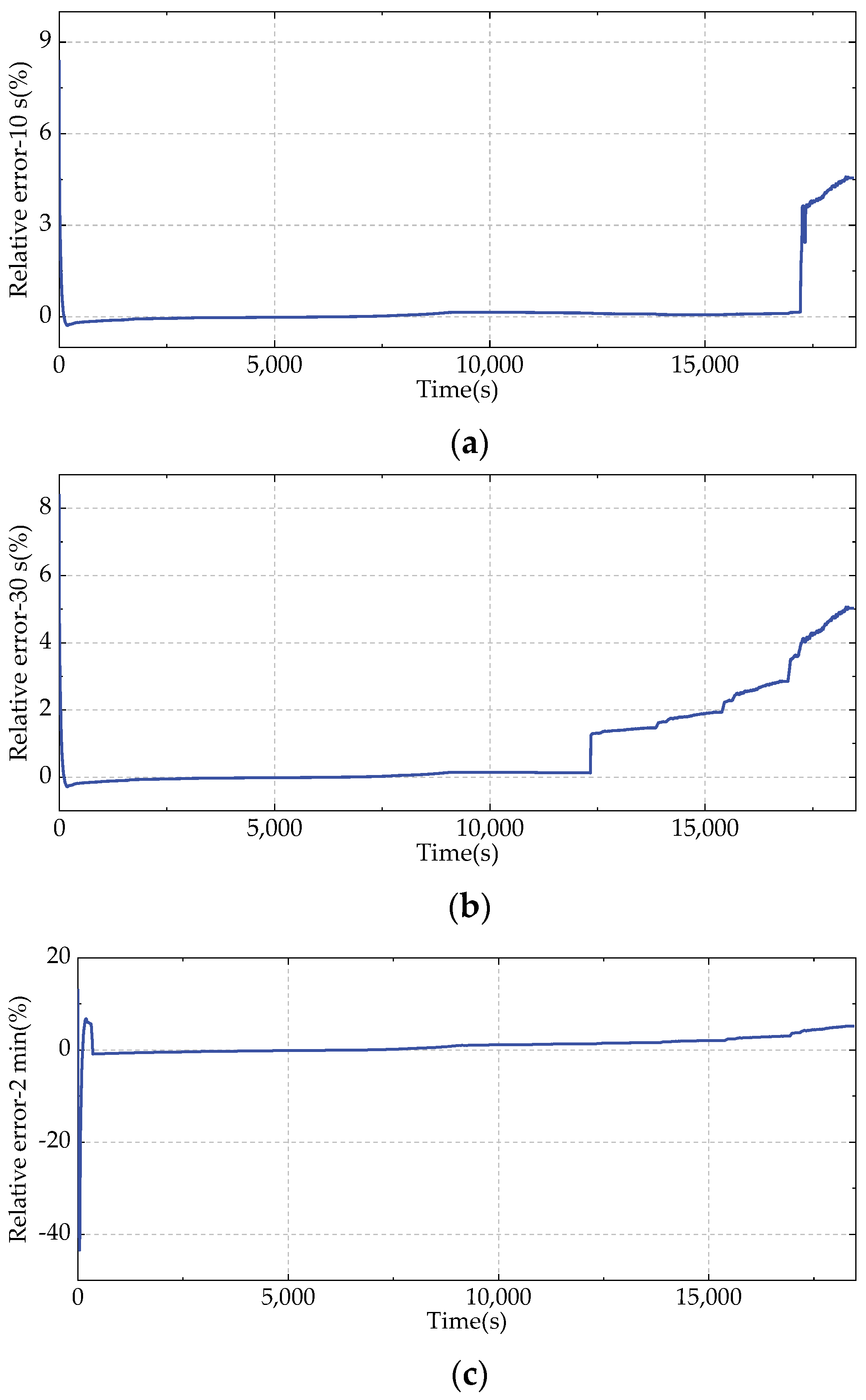
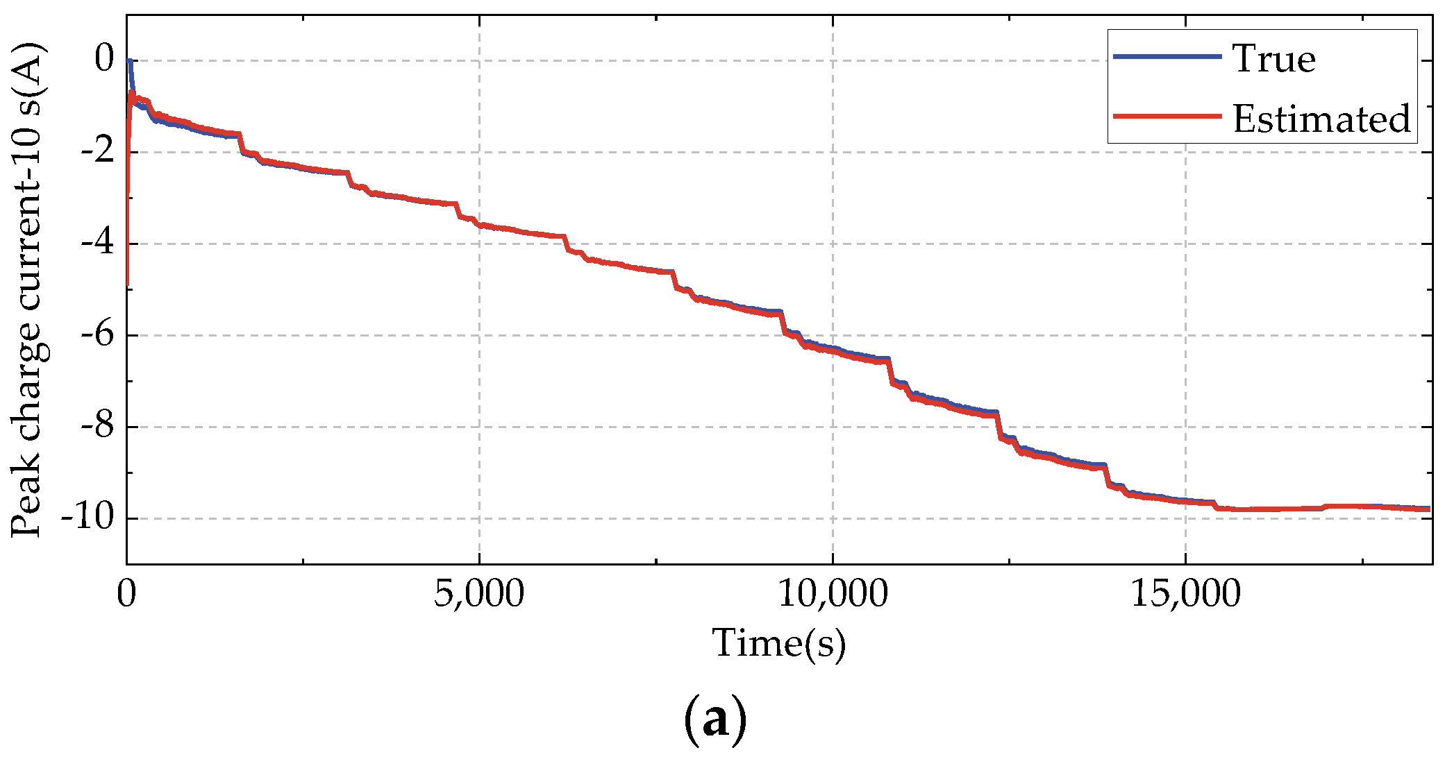
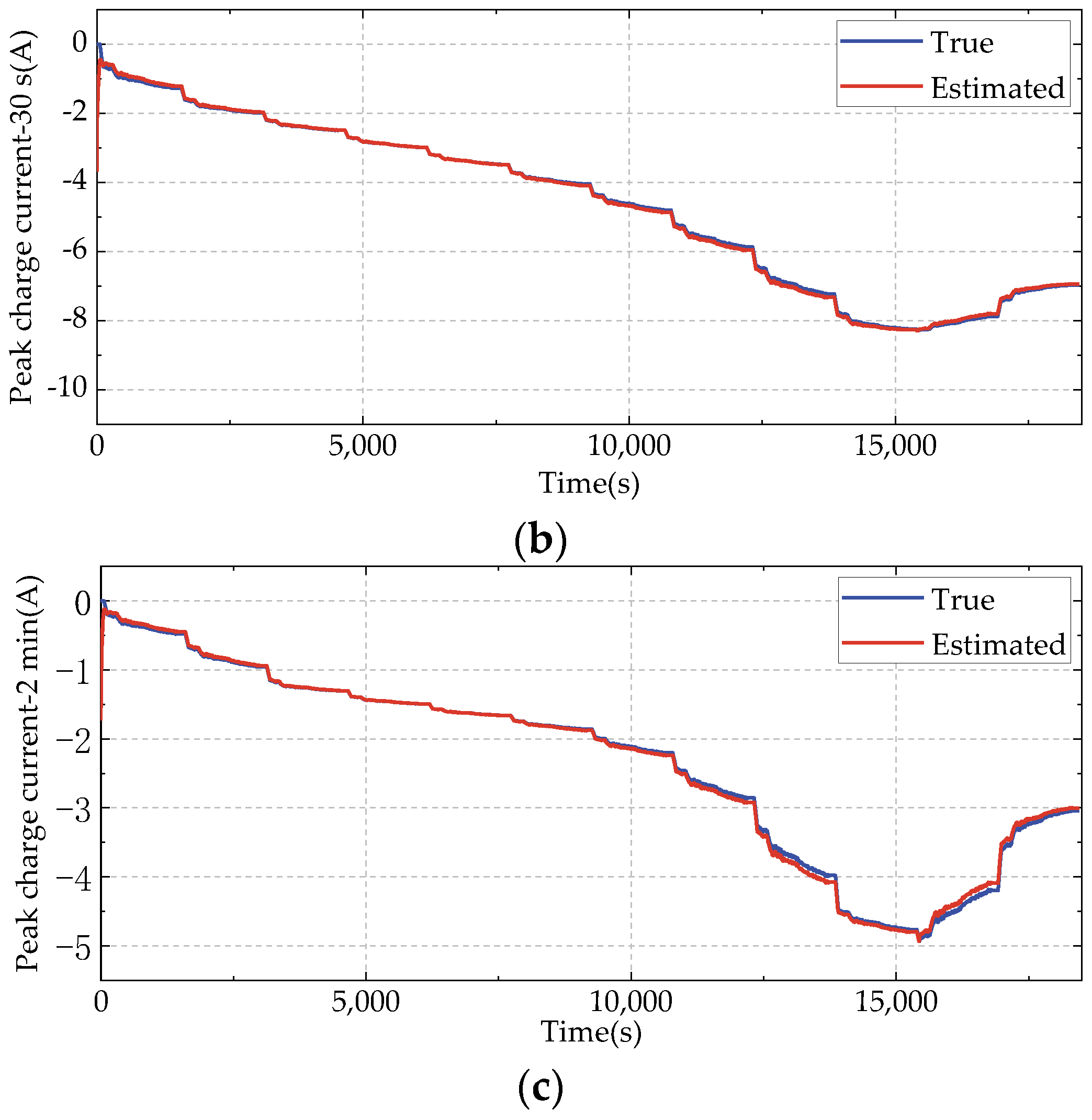
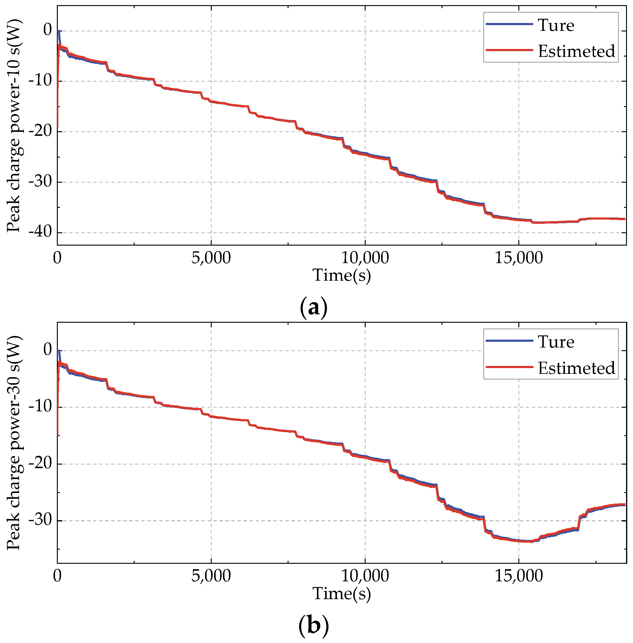
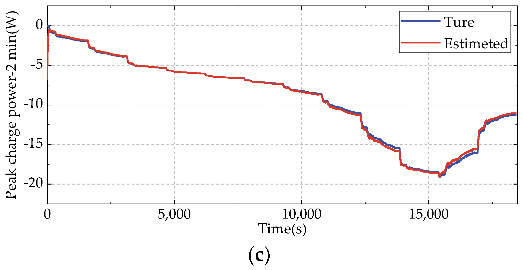
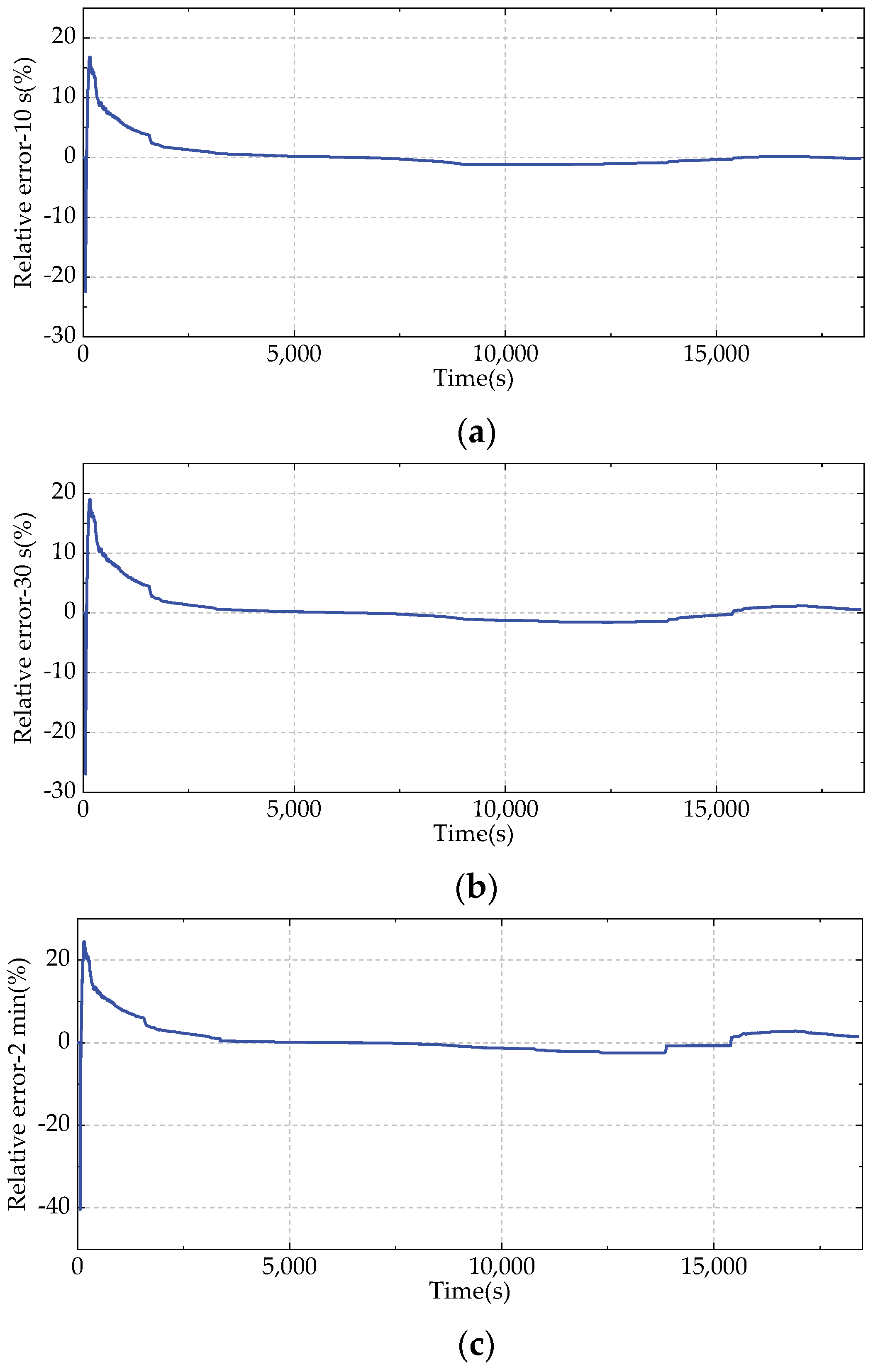
4.4.2. Charging SOP Estimation

Figure 17 and Figure 18 show the estimation results of the sustained peak charging current under different constraints for a duration of 10 s, 30 s, and 2 min. It can be seen that the sustained peak charging current estimated by the SOC or end voltage constraints alone is too large, which can lead to the overcharging of the Li–ion battery and seriously affect the battery performance and service life. The sustained peak charge current is mainly determined by the current terminal voltage of the lithium–ion battery, and this phase is gradually shortened as the charge time increases. This is due to the fact that the longer the sustained charge time, the easier it is to reach the set cutoff condition (terminal voltage charge cutoff condition, 4.2 V) at the same charge current. Then, it shifts to the current SOC constraint, due to the fact that the longer the sustained charge time, the more charge is required to reach the preset cutoff condition at the same moment. This is due to the fact that the longer the continuous charging time, the less current is required to charge at the same moment to reach the set cut-off condition. The required charging current reaches the maximum battery design charging current at a slower rate, and this phase time is shortened.

Figure 19 and Figure 20 show the continuous peak charging power curves and the corresponding error results for 10 s, 30 s, and 2 min of continuous charging. As the continuous charging time increases, the charge current required to reach the set cutoff condition (SOC charging limit condition or end-voltage charging cutoff condition) at the same moment is reduced, as is the value of the continuous peak charging power at the same moment. According to the results listed in

Table 2. Estimation errors of sustained peak charging power for different time scales.

Time Scale	RMSE (W)	MARE (%)	Title 1	Title 2	Title 3
10 s	0.9019	0.77	entry 1	data	data
30 s	1.5034	1.02	entry 2	data	data
2 min	2.2763	1.53

, the sustained peak charging power MARE at different sustained charge times is less than 1.6% and the RMSE falls within the range of 2.3 W.

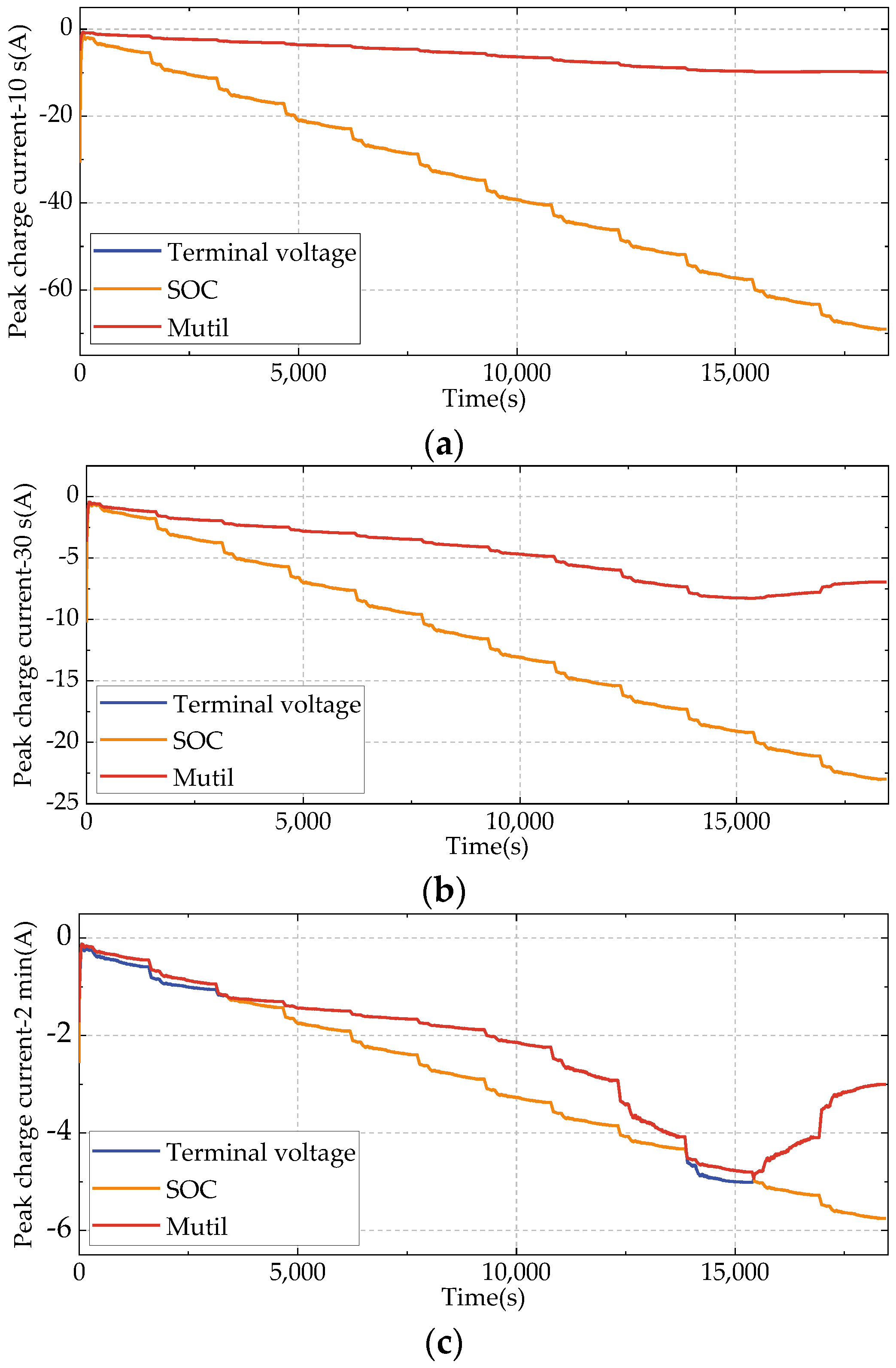
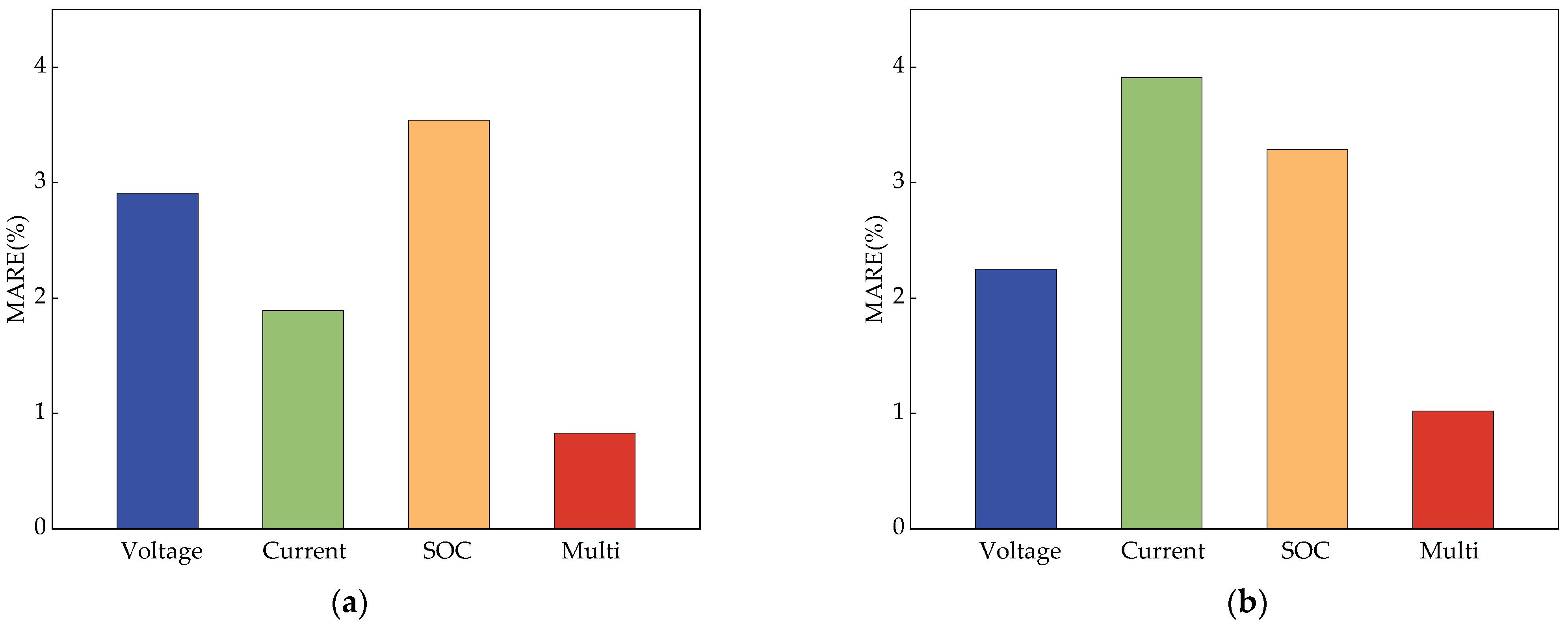
4.4.3. Comparison of SOP Estimates

As the SOP of the lithium–ion battery reflects the charging/discharging capacity of the battery, its accurate estimation can not only provide guidance on how to use the battery rationally and ensure the optimal power distribution, but also avoid the overcharging and overdischarging of the battery and extend the service life of the lithium–ion battery. From Table 1 and Table 2, it can be seen that the SOP estimation error increases with the increase in time scale, with the acceleration, climbing, and braking energy recovery process of the electric vehicle completed in a period of time. Therefore, it is necessary to consider the time scale for the accurate SOP estimation. Figure 21 shows the comparison of the relative error of the average absolute value of SOP estimation under different constraints at the time scale of 30 s. It can be seen from this figure that only a single constraint leads to overcharge and overdischarge of the battery, and the battery SOP is constrained by the common constraints of voltage, current, and SOC. Moreover, the three constraints work alternately at different stages of the charging/discharging process, and the multi-constraint SOP estimation MARE does not exceed 1.1%. In the extreme SOC state of the battery, there is a risk of overcharging and overdischarging for the battery, and the SOC limit is dominant at this stage. For this reason, the H∞ filter algorithm with evident estimation accuracy advantage as described in Section 4.3 is used for SOC estimation, and the result of this estimation is taken as a constraint for SOP estimation. The results listed in Table 1 and Table 2 show that the MARE of SOP estimation is less than 1.6% and the RMSE is less than 2.3 W.

It can be seen from the SOP calculation process in Section 3.2 that the prerequisite for calculating SOP is to calculate the peak current. The SOP value in the current time scale can be obtained by multiplying the calculated peak current and the battery terminal voltage. The peak current based on voltage constraint and SOC constraint and the terminal voltage of the battery are calculated based on the current SOC of the battery. It can be seen that the accuracy of SOC estimation is important for SOP estimation. In order to evaluate the convergence and performance of the proposed method, the EKF algorithm, UKF algorithm, and H∞ algorithm are used to jointly estimate SOC–SOP under the condition that SOC has a large initial error. Figure 22 shows the comparison diagram of charging and discharging SOP estimation based on the H∞, UKF, and EKF algorithms to estimate SOC at a 30 s time scale. From the partial enlargement of Figure 22, it can be seen that the joint SOC–SOP estimation based on the H∞ algorithm can accurately estimate the SOP in the high, middle, and low SOC intervals. The accuracy of the SOP estimation depends largely on the accuracy of the SOC estimation. When the SOC estimation does not converge, the result of the SOP estimation does not converge. From the initial stage of estimation in Figure 22, it can be seen that the given initial value of SOC has a large error, resulting in a large error in SOP estimation. With the rapid convergence of SOC under the H∞ algorithm, SOP also converges rapidly. It can be seen that the convergence of SOC affects the convergence of SOP. From

Table 3. Convergence time of charge and discharge SOP estimation of SOC based on H∞, UKF, and EKF algorithm in 30 s time scale.

Technique	Discharge (s)	Charge (s)
H∞	80	90
UKF	821	1088
EKF	1426	1605

, we can see that the convergence time of joint SOC–SOP estimation based on the H∞ algorithm is less than 100 s, and its effect is far greater than that of joint SOC–SOP estimation based on the EKF algorithm or the UKF algorithm.

5. Conclusions

The accurate management of lithium–ion batteries plays a key role in not only the safe and reliable operation of electric vehicles, which requires the accurate estimation of lithium–ion battery state, but also the effective monitoring and control, which mainly involves SOC estimation and SOP estimation of lithium–ion batteries. In this paper, the focus of study is placed on three aspects: model parameter identification, SOC estimation, and the SOP estimation of the power lithium–ion battery.

(1)

To address the significant computational workload required by traditional online identification methods, it is proposed in this paper to address the online identification of model parameters through the recursive least squares method with forgetting factor, which achieves a high accuracy and a strong tracking capability under the condition of low computational workload;

(2)

To eliminate the unavoidable measurement noise from current, voltage, and other sensors, H∞ filtering is performed for process noise and measurement noise. SOC estimation is also carried out;

(3)

To resolve problems such as insufficient constraints, the low accuracy of SOC estimation, and single time scale, a multi-constraint SOP estimation method based on multiple time scales is proposed in this paper.

It is verified under the context of UDDS that the H∞ filtering algorithm still performs well in tracking the SOC reference value changes when the initial value of SOC shows a large error, which is evidently superior to the EKF algorithm and the UKF algorithm. The estimated MARE of SOC is less than 1.5%, and the RMSE is less than 0.5%. Based on high-precision SOC, the multi-constrained charge and discharge SOP is estimated to have a MARE of less than 1.6% and an RMSE of less than 2.5 W at two different time scales: 10 s, 30 s, and 2 min. The verification results show the high accuracy and strong robustness of the proposed multi-time scale lithium–ion battery SOP estimation method based on H∞ filtering. As the changes in temperature and parameters (internal resistance and capacity) are ignored in this paper, the accuracy of SOP estimation is affected. For example, a temperature rise accelerates the internal side reactions of lithium batteries [31,32]. The reduction in temperature causes active lithium to deposit on the electrode surface, which affects the available capacity, internal resistance, and other characteristic parameters of the lithium battery [33,34,35]. In future studies, temperature and aging conditions will be taken into account for SOP estimation.

References

1. Jin, X.N.; Gu, Q.M.; Pan, Y.W.; Hua, Y. Online state of power estimation methods for lithium-ion batteries in EV. China J. Power Sources 2019, 43, 1448–1452. [Google Scholar]
2. Xiong, R.; Sun, F.C.; Gong, X.Z. A data-driven based adaptivestate of charge estimator of lithium-ion polymer battery used inelectric vehicles. Appl. Energy 2014, 113, 1421–1433. [Google Scholar] [CrossRef]
3. Wen, G.B.; Rehman, S.; Tranter, T.G.; Ghosh, D.; Chen, Z.; Gostick, J.T.; Pope, M.A. Insights into Multiphase Reactions during Self-Discharge of Li-S Batteries. Chem. Mater. Publ. Am. Chem. Soc. 2020, 32, 4518–4526. [Google Scholar] [CrossRef]
4. Bhattacharjee, A.; Mohanty, R.K.; Ghosh, A. Design of an optimized thermal management system for Li-Ion batteries under different discharging conditions. Energies 2020, 13, 5695. [Google Scholar] [CrossRef]
5. Liu, X.T.; He, Y.; Zeng, J.G.; Zheng, X.X. State-of-Power estimation for Li-ion battery considering the effect of temperature. Trans. China Electrotech. Soc. 2016, 31, 155–163. [Google Scholar]
6. Yoon, S.; Hwang, I.; Lee, C.W.; Ko, H.S.; Han, K.H. Power capability analysis in lithium ion batteries using electrochemical impedance spectroscopy. J. Electroanal. Chem. 2011, 655, 32–38. [Google Scholar] [CrossRef]
7. Chen, C.; Pi, Z.Y.; Zhao, Y.L.; Liao, X.; Zhang, M.M. State of charge estimation with adaptive cataclysm genetic algo-rithm-recurrent neural network for Li-ion batteries. J. Electr. Eng. 2022, 17, 86–94. [Google Scholar]
8. Qian, J.W.; Du, C.; Tian, X.; Zhu, Y.B. An improved fuzzy neural network method based on T-S model to estimate state of charge of lithium batteries. China J. Power Sources 2020, 44, 1270–1273. [Google Scholar]
9. Tang, X.; Liu, K.; Li, K.; Widanage, W.D.; Kendrick, E.; Gao, F. Recovering large-scale battery aging dataset with machine learning. Patterns 2021, 2, 1000302. [Google Scholar] [CrossRef]
10. Li, W.; Sengupta, N.; Dechent, P.; Howey, D.; Annaswamy, A.; Sauer, D.U. One-shot battery degradation trajectory prediction with deep learning. J. Power Sources 2021, 506, 230024. [Google Scholar] [CrossRef]
11. Mastali, M.; Vazquez-Arenas, J.; Fraser, R.; Fowler, M.; Afshar, S.; Stevens, M. Battery state of the charge estimation using Kalman filtering. J. Power Sources 2013, 239, 294–307. [Google Scholar] [CrossRef]
12. Huang, C.; Wang, Z.; Zhao, Z.; Wang, L.; Lai, C.S.; Wang, D. Robustness evaluation of extended and unscented kalman filter for battery state of charge estimation. IEEE Access 2018, 6, 27617–27628. [Google Scholar] [CrossRef]
13. Andre, D.; Appel, C.; Soczka-Guth, T.; Sauer, D.U. Advanced mathematical methods of SOC and SOH estimation for lithium-ion batteries. J. Power Sources 2013, 224, 20–27. [Google Scholar] [CrossRef]
14. Xiong, R.; Cao, J.Y.; Yu, Q.Q.; He, H.W.; Sun, F.C. Critical review on the battery state of charge estimation methods for electric vehicles. IEEE Access 2017, 6, 1832–1843. [Google Scholar] [CrossRef]
15. Xiong, R.; He, H.W.; Sun, F.C.; Liu, X.L.; Liu, Z.T. Model-based state of charge and peak power capability joint estimation of lithium-ion battery in plug-in hybrid electric vehicles. J. Power Sources 2013, 229, 159–169. [Google Scholar] [CrossRef]
16. Li, W.; Fan, Y.; Ringbeck, F.; Jöst, D.; Han, X.; Ouyang, M.; Sauer, D.U. Electrochemical model-based state estimation for lithium-ion batteries with adaptive unscented Kalman filter. J. Power Sources 2020, 476, 228534. [Google Scholar] [CrossRef]
17. Wang, T.; Chen, S.; Ren, H.; Zhao, Y. Model-based unscented Kalman filter observer design for lithium-ion battery state of charge estimation. Int. J. Energy Res. 2012, 42, 1603–1614. [Google Scholar] [CrossRef]
18. Zou, C.; Klintberg, A.; Wei, Z.; Fridholm, B.; Wik, T.; Egardt, B. Power capability prediction for lithium-ion batteries using economic nonlinear model predictive control. J. Power Sources 2018, 396, 580–589. [Google Scholar] [CrossRef]
19. Sun, B.X.; Gao, K.; Jiang, C.J.; Luo, M.; He, T.T.; Zheng, F.D.; Guo, H.Y. Research on discharge peak power prediction of battery based on ANFIS and subtraction clustering. Trans. China Electrotech. Soc. 2015, 30, 272–280. [Google Scholar]
20. Zhu, H.; Zhang, W.B.; Deng, Y.W.; Li, M.; Ji, X. Peak power estimation of power battery discharge based on SA + BP hybrid algorithm. J. Jiangsu Univ. 2020, 41, 192–198. [Google Scholar]
21. Plett, G.L. High-performance battery-pack power estimation using a dynamic cell model. IEEE Trans. Veh. Technol. 2004, 53, 1586–1593. [Google Scholar] [CrossRef] [Green Version]
22. Xavier, M.A.; de Souza, A.K.; Plett, G.L.; Trimboli, M.S. A low-cost MPC-based algorithm for battery power limit estimation. In Proceedings of the 2020 American Control Conference (ACC), Denver, CO, USA, 1–3 July 2020; pp. 1161–1166. [Google Scholar]
23. Zhang, W.; Shi, W.; Ma, Z. Adaptive unscented Kalman filter based state of energy and power capability estimation approach for lithium-ion battery. J. Power Sources 2015, 289, 50–62. [Google Scholar] [CrossRef]
24. Pei, L.; Zhu, C.; Wang, T.; Lu, R.; Chan, C.C. Online peak power prediction based on a parameter and state estimator for lithium-ion batteries in electric vehicles. Energy 2014, 66, 766–778. [Google Scholar] [CrossRef]
25. Tang, X.; Wang, Y.; Yao, K.; He, Z.; Gao, F. Model migration based battery power capability evaluation considering uncertainties of temperature and aging. J. Power Sources 2019, 440, 227141. [Google Scholar] [CrossRef]
26. Zhang, W.J.; Wang, L.Y.; Wang, L.F.; Liao, C.L.; Zhang, Y.W. Joint State-of-Charge and State-of-Available-Power Estimation Based on the Online Parameter Identification of Lithium-Ion Battery Model. IEEE Trans. Ind. Electron. 2022, 69, 3677–3688. [Google Scholar] [CrossRef]
27. Guo, R.H.; Shen, W.X. A data-model fusion method for online state of power estimation of lithium-ion batteries at high discharge rate in electric vehicles. Energy 2022, 254, 124270. [Google Scholar] [CrossRef]
28. Hu, X.S.; Jiang, H.; Feng, F.; Liu, B. An enhanced multi-state estimation hierarchy for advanced lithium-ion battery management. Appl. Energy 2020, 257, 114019. [Google Scholar] [CrossRef]
29. Dong, G.; Wei, J.; Chen, Z. Kalman filter for onboard state of charge estimation and peak power capability analysis of lithium-ion batteries. J. Power Sources 2016, 328, 615–626. [Google Scholar] [CrossRef]
30. Rahimifard, S.; Ahmed, R.; Habibi, S. Interacting multiple model strategy for electric vehicle batteries state of charge/health/power estimation. IEEE Access 2021, 9, 109875–109888. [Google Scholar] [CrossRef]
31. Li, Q.; Wang, T.; Li, S.; Chen, W.; Liu, H.; Breaz, E.; Gao, F. Online extremum seeking-based optimized energy management strategy for hybrid electric tram considering fuel cell degradation. Appl. Energy 2021, 285, 116505–118153. [Google Scholar] [CrossRef]
32. Shrivastava, P.; Soon, T.K.; Idris, M.Y.I.B.; Mekhilef, S. Overview of model-based online state-of-charge estimation using Kalman filter family for lithium-ion batteries. Renew. Sustain. Energy Rev. 2019, 113, 109233. [Google Scholar] [CrossRef]
33. Mevawalla, A.; Panchal, S.; Tran, M.K.; Fowler, M.; Fraser, R. One dimensional fast computational partial differential model for heat transfer in lithium-ion batteries. J. Power Sources 2021, 37, 102471. [Google Scholar] [CrossRef]
34. Yang, N.; Song, Z.; Hofmann, H.; Sun, J. Robust state of health estimation of lithium-ion batteries using convolutional neural network and random forest. J. Energy Storage 2022, 48, 103857. [Google Scholar] [CrossRef]
35. Li, X.; Wang, Z.; Zhang, L. Co-estimation of capacity and state-of-charge for lithium-ion batteries in electric vehicles. Energy 2019, 174, 33–44. [Google Scholar] [CrossRef]
Figure 1. Battery state estimation methods classification.
Batteries 09 00191 g001
Figure 2. Model structure of 2-RC equivalent circuit.
Batteries 09 00191 g002
Figure 3. Schematic diagram of forgetting factor recursive least squares (FFRLS).
Batteries 09 00191 g003
Figure 4. SOC estimation process.
Batteries 09 00191 g004
Figure 5. SOP estimation process.
Batteries 09 00191 g005
Figure 6. Battery testing system.
Batteries 09 00191 g006
Figure 7. Excitation current under UDDS condition.
Batteries 09 00191 g007
Figure 8. Experimental data and fitting curve of OCV–SOC.
Batteries 09 00191 g008
Figure 9. Parameter identification results of FFRLS algorithm under UDDS condition: (a) R0, R1, R2; (b) C1, C2.
Batteries 09 00191 g009
Figure 10. Terminal voltage response and relative error of FFRLS parameter identification under UDDS condition: (a) estimated terminal voltage; (b) corresponding error of terminal voltage estimation.
Batteries 09 00191 g010
Figure 11. The results of SOC and voltage estimation using different methods under UDDS conditions: (a) SOC estimation results; (b) terminal estimation results.
Batteries 09 00191 g011
Figure 12. Error of SOC estimation by H∞ algorithm under UDDS condition.
Batteries 09 00191 g012
Figure 13. Results of multi-constraint peak discharge current estimation in different time scales: (a) 10 s; (b) 30 s; (c) 2 min.
Batteries 09 00191 g013aBatteries 09 00191 g013b
Figure 14. Results of peak discharge current estimation in different time scales: (a) 10 s; (b) 30 s; (c) 2 min.
Batteries 09 00191 g014
Figure 15. Results of peak discharge power estimation: (a) 10 s; (b) 30 s; (c) 2 min.
Batteries 09 00191 g015
Figure 16. Results of peak discharge power relative error: (a) 10 s; (b) 30 s; (c) 2 min.
Batteries 09 00191 g016
Figure 17. Results of multi-constraint peak charge current estimation in different time scales: (a) 10 s; (b) 30 s; (c) 2 min.
Batteries 09 00191 g017
Figure 18. Results of peak charge current estimation in different time scales: (a) 10 s; (b) 30 s; (c) 2 min.
Batteries 09 00191 g018aBatteries 09 00191 g018b
Figure 19. Results of peak charge power estimation: (a) 10 s; (b) 30 s; (c) 2 min.
Batteries 09 00191 g019aBatteries 09 00191 g019b
Figure 20. Results of peak charge power relative error: (a) 10 s; (b) 30 s; (c) 2 min.
Batteries 09 00191 g020
Figure 21. 30 s SOP estimation MARE with different constraints: (a) discharge; (b) charge.
Batteries 09 00191 g021
Figure 22. Comparison of charge and discharge SOP estimation based on H∞, UKF, and EKF algorithm to estimate SOC in 30 s time scale: (a) discharge; (b) charge.
Batteries 09 00191 g022