1. Introduction
With growing concern over the environment and the greenhouse effect, EVs are gradually becoming the focus of attention. Lithium-ion batteries are widely applied for the power system of EVs due to their excellent performance, i.e., high energy density, high voltage and long life [
1,
2,
3,
4]. Lithium-ion batteries are easily influenced by ambient temperature, charge and discharge rate, aging and other factors under operations [
5,
6,
7]. It is essential to establish a reliable battery management system (BMS) to monitor and predict the battery state with high-accuracy and real-time [
8,
9]. Among the states of batteries, the battery state of charge represents the ratio of the remaining usable capacity of the battery to the applicable current maximum capacity, which is one of the key states of the battery. Accurate and real-time SOC information determines the range and ensure the reliability of the battery operation by BMS [
10]. However, the battery is a highly complex electrochemical system with time-varying and non-linear characteristics because of the complex electrochemical dynamics and multi-physical field coupling inside the battery [
11,
12,
13]. Therefore, it is still a significant task to accurately estimate SOC online based on macroscopic signals.
At present, the essential SOC estimation methods include: 1. the coulomb counting method (CCM), 2. the open-circuit-voltage (OCV) method, 3. the model-based method and 4. the data-driven method.
The coulomb counting method integrates the measured current with time, while monitoring the real-time SOC of the battery online based on the initial SOC. This method is equipped with the ease of implementation, but the initial error will affect the accuracy seriously. Additionally, such method is an open-loop method, where the cumulative error influences the SOC error [
14].
By establishing the corresponding relationship between the OCV and SOC, the OCV method can map the SOC of the battery by obtaining the OCV [
15,
16]. However, the OCV-SOC relationship will be influenced by temperature and degradation. If the relationship is not updated in time, serious SOC estimation errors may result. Moreover, when the SOC is in the middle range (20–80%), the OCV-SOC characteristic curve will present a flat plateau, especially in lithium iron phosphate (LFP) batteries. At this time, the small error of OCV will sharply increase the estimation error of SOC, which will cause the estimation to be very sensitive. In addition, when measuring OCV, it is necessary to disconnect the battery for a certain period of time (more than 2 h) to make it reach a stable state to ensure accuracy. Therefore, this method is only applicable to specific application scenario such as laboratories, and cannot achieve the requirements of onboard applications [
17].
The model-based method is mainly implemented through three steps: battery modelling, parameter identification and state estimation. At present, most of the model-based methods used in practice are to establish an equivalent circuit model (ECM) and identify the parameters, and then estimate the SOC through Kalman’s filter or other observers [
18]. The model-based method belongs to a closed-loop system, which can reduce the interference of uncertainty through self-tuning. It has robustness to initial SOC offset and measurement noise and has achieved high estimation accuracy under specific operating conditions. Plett applied extended Kalman filters (EKF) and different battery models in BMS to estimate the SOC for lithium polymer batteries [
19,
20,
21]. Based on the cubature Kalman filter (CKF), Peng et al. [
22] achieved SOC estimation with high-accuracy and robustness by establishing an equivalent circuit model and identifying the parameters using the Sequential Quadratic Programming (SQP) method, which shows that CKF is more accurate than EKF in estimating the SOC of lithium batteries. Ling et al. [
23] proposed an estimation method based on the probability fusion of ACKF and AHCKF to further improve the estimation accuracy and robustness of SOC. However, although the method based on the ECM model can achieve better accuracy and robustness with relatively small calculation consumption, it is usually difficult to establish an accurate model because of the changes in the internal resistance and capacitance of the battery for different battery aging process and different temperatures in practical applications, and the OCV-SOC look-up tables will also be affected by different battery aging process and different temperatures, such error will increase if the update is not timely.
The data-driven method is not constrained by the physical relationship, which is easier to establish a high-efficient model. The non-linear relationship between SOC and measurable signals such as current, voltage and temperature can be established by training a substantial number of sample data. With appropriate training, higher estimation accuracy can be achieved [
24]. At the same time, the battery SOC estimation model established based on the data-driven method has a strong generalization in different working environments of the battery. Chaoui et al. [
25] realized the estimation of battery SOC through a recurrent neural network (RNN), but ordinary RNN cannot solve the long-term dependence problem. Chemali et al. [
26] used the Long short-term memory (LSTM) to achieve the estimation of SOC with high accuracy, and the same model can be applied at different temperatures, overcoming the problem that model parameters need to be updated due to changes in the working conditions. One-dimensional convolution also has an excellent performance in solving time series problems. Hannan et al. [
27] realized high-accuracy SOC estimation by using a one-dimensional depth full convolution network with a learning rate optimization algorithm. In general, the data-driven method still has problems such as large computation consumption and limited accuracy. The data-driven method is significantly dependent on the quality and quantity of the data. When the specific working conditions of a specific battery are used as training data, because the training data cannot fully reflect the inherent characteristics of the battery, large estimation errors may occur in different battery systems and under the complex and dynamic working conditions of the battery. Meanwhile, when the amount of data is large, the training of data-driven models requires a huge computing cost.
Obviously, each individual method has its own drawbacks when using a single method to estimate the battery SOC. Collaboration between various approaches is an effective solution to obtain more accurate results. Tian et al. [
28] extracted the open circuit voltage (OCV), ohmic response and polarization voltage from the voltage and current sequence as features and input them into the deep neural network (DNN) for battery SOC estimation. Feng et al. [
29] fused the simplified single particle model (SSPM) with the thermal model to form a lumped model to estimate the battery SOC through the unscented Kalman filter (UKF), and used the feedforward neural network to improve the performance of the lumped model under an extreme working environment. Ragone et al. [
30] combined a vehicle model, an electrochemical degradation model, a battery thermal model and a machine learning to estimate the SOC for the EVs. Although the method of model collaboration can achieve high accuracy, the constructed model has a high degree of complexity, which will increase calculation consumption and is unsuitable for vehicle applications. At the same time, many collaboration models still have the problem of generalization under different temperatures.
In summary, there are several main issues in the estimation of battery SOC: one is that the generalization of the estimation of SOC is weak under various working conditions, especially for temperature conditions, and the impact will become more critical with battery degradation and inconsistency. It is essential to update the model parameters in a timely manner to ensure accuracy under different temperatures, but in the data-driven method, the temperature can be simply regarded as a feature and directly input into the model for training and prediction, which greatly reduces the difficulty of the operation and effectively solves the problem of SOC estimation under different temperatures. Another problem is the contradiction between the constrained computing power of vehicle terminals in practical applications and the requirements for accurate algorithms functional in real-time. The high-accuracy results of most methods are usually obtained by building complex models. However, in practical applications, excessive computing consumption may lead to slow signal response time, which cannot guarantee the real-time performance of SOC estimation due to the constraint computing power of the onboard BMS. Although some methods also have high computing efficiency, these methods are all aimed at predicting battery cells and cell only. In practical applications, the electric vehicles are equipped with battery packs, which leads to the calculation consumption multiplied, where the problems mentioned above still stand.
In order to deal with the above problems, this paper proposes an end-cloud collaboration approach to online estimate SOC. The deep learning model can directly input the simple temperature as a feature into the network for training and prediction, which solves the problem of generalization under different temperatures, and the end-cloud collaborative working mode can share the calculation consumption, so as to solve the contradiction between accuracy and real-time. The deep learning model with large calculation consumption is deployed on the cloud-side and the real-time collected measurable signals are uploaded to the cloud for offline estimation. The data-driven model on the cloud-side is built with the CNN-LSTM network as the core. This model can effectively deal with the time series problem of SOC estimation in the battery, a non-linear system, and can obtain satisfactory estimation accuracy under different temperatures. The state function constructed by the coulomb counting method with less calculation consumption is deployed on the end-side, and the online calculation is carried out through the real-time collected current. At the same time, the Kalman filtering algorithm is deployed on the end-side to fuse the estimation results of the cloud-side and end-side, to achieve high-accuracy and real-time SOC online estimation. The accuracy and robustness of the proposed end-cloud collaboration approach were evaluated with three dynamic driving conditions, including dynamic stress test (DST), US06 driving schedule and federal urban driving schedule (FUDS) under different temperatures and different initial errors.
This paper is organized as follows:
Section 2 shows the theory of the models and algorithms deployed on the cloud-side and end-side, as well as the structure of the whole end-cloud collaboration system.
Section 3 describes the settings of software and hardware in the experiment and the evaluation index of the experiment.
Section 4 describes the estimation results and discussions of the proposed method. Finally,
Section 5 summarizes the main conclusions.
2. Methodology
The proposed end-cloud collaboration approach consists of three parts:
(1) Deep learning model on the cloud-side, which has high accuracy, poor real-time performance and large computing consumption, and is suitable for cloud computing.
(2) The state function constructed by the coulomb counting method on the end-side, whose accuracy is susceptible to the interference of initial value deviation, with poor accuracy and robustness, but the calculation cost is small, which is suitable for the arrangement of the end-side for calculation.
(3) Fusion algorithm. Kalman’s filtering algorithm is used to combine the result of the end-side with that of the cloud-side to obtain more accurate results.
2.1. Data-Driven Model on Cloud
The deep learning model on the cloud-side used in this paper is constructed with the CNN-LSTM model as the base.
2.1.1. CNN-LSTM Introduction
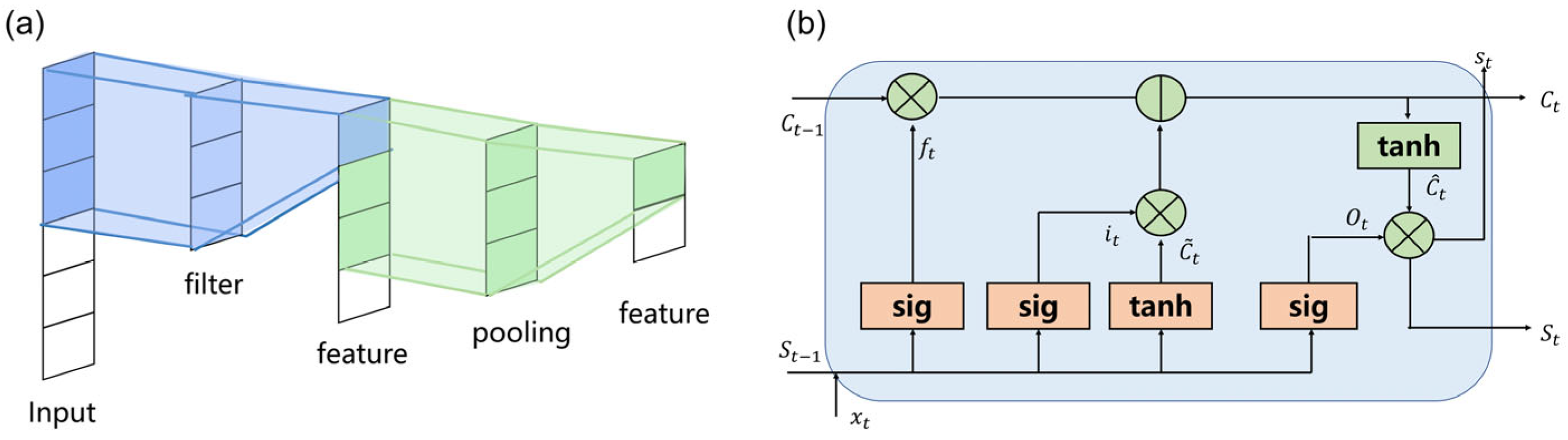
CNN and LSTM are two commonly used networks in deep learning. CNN is mainly composed of convolution layer and pooling layer, which can extract potential features from sample data through the convolution kernel, and there is an activation function after the convolution layer to introduce the nonlinear characteristics to the model [
31]. CNN has the characteristics of weight sharing and local connection, which can significantly reduce the number of model parameters, speed up training and improve generalization performance. One-dimensional CNN is mainly used in timeseries problems and the structure is shown in
Figure 1a. The one-dimensional convolution is calculated as:
where ∗ is the convolution operation,
is the
convolution map of the layer
,
is the activation function,
is the number of convolution maps,
is the weight of the operation
of the convolution kernel
of layer
and
is the offset of the convolution kernel
corresponding to the layer
.
LSTM is a variant of RNN, which adds input gates, output gates and forgetting gates to the hidden layer, and adds cells for memory storage, which can process the time series problem of long-term dependence [
32]. The schematic of a unit is shown in
Figure 1b. Each unit of LSTM can be expressed as follows:
Firstly, the LSTM units receive the
and
and the forget gate is used to control which information to be forgotten in the cell state:
where sigmoid is a nonlinear activation function, and will limit the value to the range of 0 to 1, which determines the proportion of forgotten information and update the unit status
.
Secondly, the input gate processes the input data of the current sequence position and determines which information to be updated to update the cell state. The input gate includes two parts: one uses the sigmoid activation function to determine which new information in the input is added to the cell state, and after determining the reserved input new information, the tanh activation function is used to generate new candidate vectors, and then input the information to be reserved into the cell state. The input gate can be described as follows:
Next, after determining the output of the forgetting gate and the input gate, the unit state update from
to
:
where
is the information that to be retained
is the new information to add. The sum of the two is the cell state of this sequence.
Finally, using the sigmoid activation function to determine which part of the content needs to be output, then use the tanh activation function to process the cell state, and then multiply the two parts to obtain the final output:
where
is the new hidden state, and the
is the unit state.
SOC estimation is a typical time series estimation problem but it is aimed at highly complex dynamic conditions and requires high real-time, which causes the difficulty to further extract features from the data. CNN can extract the potential features from sample data, while LSTM can capture the long-term dependence in time series problems, which has great advantages in processing time series data. Therefore, we use a hybrid model that adopts LSTM as the backend of CNN, which is called CNN-LSTM, in which CNN is used to extract features from data and LSTM is used to learn the time dependency relationship.
2.1.2. Structure of Deep Learning Model
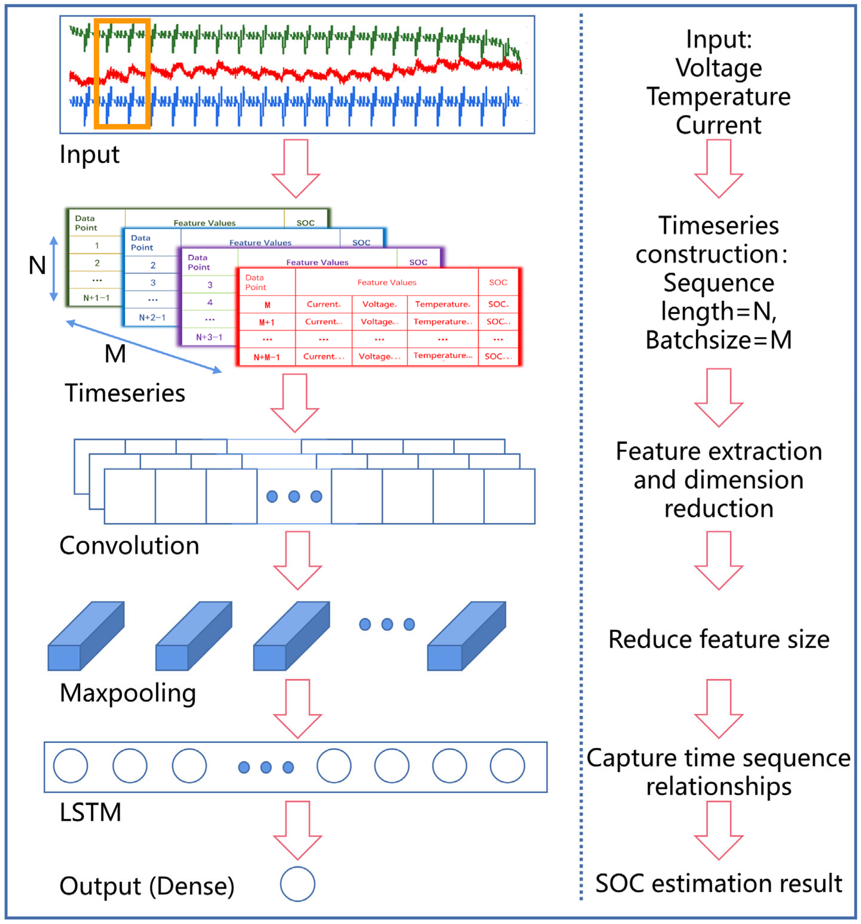
The model is constructed with the input layer, Conv1d layer, Maxpooling layer, LSTM layer and full connection layer. Since we are dealing with one-dimensional time series problems, one-dimensional convolution is used for the convolution layer. The architecture of the CNN-LSTM is shown in
Figure 2. The current, voltage and temperature are used as the input. Since the input structure required by 1d-CNN-LSTM is a 3d-tensor, the input data is built into a time series format. First, build a time series according to a certain time series length
. The input and the output structures are “many to one”. Considering that the transmission delay in practical applications will affect the real-time performance, this work focuses on the SOC estimation of the future time step, that is, extrapolating the SOC of the future time based on historical data. The input and output of the CNN-LSTM can be described as follows:
where
,
and
are the current, voltage and temperature, respectively.
is the SOC at time
, where
is the extrapolation step size and is selected as 1 in this paper.
is the input matrix of CNN-LSTM and
is the output of CNN-LSTM at time
.
Generally, a longer time series length will improve the accuracy of the estimation but will reduce the efficiency of the model. For the sake of real-time, it is not appropriate to choose too large a time series. After comprehensive consideration of model accuracy and model efficiency and debugging, the time series length is selected as 300. The constructed time series is constructed into a batch according to the batch size subsequently. With the increase of the batch size, the training speed will be accelerated, but model will converge to the local optimal point easily. After comprehensive consideration of the model efficiency and prediction accuracy, the batch size is selected as 2560. Then, the input data is processed through CNN; with the operation of convolution and pooling, CNN extracts features from input and reduces the feature dimension. The convolution layer extracts potential features from the original data through the sliding of the filter in the time dimension. The pooling layer uses maxpooling, and the processing of the pooling layer can further reduce the feature size to reduce the amount of computation. After that, the LSTM receives the data processed by CNN and the LSTM network adjust the parameters in each gate through training so that it can learn the time-dependence relationship between data from features extracted by the CNN, thus effectively solving the time series prediction problems. Finally, the predicted value is output by the full connection layer, and the sigmoid activation function is added to the full connection layer. The detailed training and testing process can be found in
Figure S1 and Table S1.
2.2. CCM in End
The state function constructed by CCM is deployed at the end-side. The change in charge is obtained through integrating the current with time, the coulomb counting method is calculated as:
where
is the rated capacity of the battery,
is the current and
is the charge and discharge efficiency.
When the CCM is carried in vehicle BMS, it needs to be discretized first. In addition, the integration of the cloud-side model and the end-side also needs the discrete form, which can be described as follows:
where
is the time interval between time
and time
,
is the current at time
,
is the SOC at time
obtained by the CCM and
is the SOC at time
obtained through the CCM. This method has a clear physical basis and simple calculation, and consumes little computational resources. However, as an open-loop method, it is easy to encounter the influence of cumulative error, so it is necessary to use certain methods to correct it in practical application.
2.3. End-Cloud Collaboration
Kalman’s filter algorithm is deployed on the end-side for fusion. The KF algorithm estimates the system state based on the linear system state function through the input and output observation data of the system, but only linear systems can adopt the KF algorithm. The UKF algorithm is an improvement on the KF algorithm, which adopts the Kalman linear filtering framework and approximates the probability density of nonlinear functions based on the Bayesian transform and UT transform. The UKF algorithm has high accuracy in nonlinear problems, and can also be applied to linear problems. Although the state function and measurement function constructed in the application of this paper are all linear functions, considering that the follow-up work will be extended to the joint estimation of multi-state quantities, in order to deal with the possible nonlinear problems, this paper will adopt the KF and UKF algorithms, respectively, as collaborative algorithms, and make a comparison between these two algorithms, to explore the impact of the approximate transformation of the UKF on the accuracy.
2.3.1. KF Algorithm
The Kalman filter is a filtering algorithm based on optimal estimation [
33]. By comprehensively considering estimated values and measured values, it fuses state variables and observation variables to get a result close to real value, which will as state variables of the next process, and then fuses with the observation variables of the next process, so iteratively. The KF algorithm can be described as follows:
Expression (12) is a state function, where represents the current state, represents the previous state, represents the input, represents the process noise, and B represent the state transition matrix. Expression (13) is a measurement function, where represents measured variables, represents measurement noise and represents the transfer parameters matrix of the measured variables. The working process of Kalman filter is as follows:
where
is the prior estimate of the state,
is the posteriori optimal estimate,
is the prior estimates of covariance,
is the posterior optimal estimation of the covariance,
is the Kalman gain and
is a complete identity matrix.
2.3.2. UKF Algorithm
The UKF is a method that enables nonlinear problems to be applied to the KF system only applicable to linear problems through UT transformation [
34]. The UKF algorithm can be described as follows:
where,
is the system noise, and
is the measurement noise.
The process of UKF algorithm is as follows:
First determine the initial value of the status value
and the initial covariance of the status error
, and then calculate the sampling points:
The weight value is calculated as follows:
where
is the scale factor between the mean of random variable
and the sigma sampling points,
is the row
or column
of the square root matrix obtained by Cholesky decomposition of matrix
,
and
are the scale factor, and
is a high-order characteristic reflecting the state history information.
Then update the prior status value
and system variance prediction value
:
where
is the system noise covariance matrix. Next, update the observations
and predicted value of observation variance
.
Finally, update the covariance
, the posterior state value
and the posterior state error covariance
.
2.3.3. Collaboration Process
For the SOC estimation, the state vector is
, which follows the coulomb counting method to construct the state function and deploy on the end-side. The measurement vector is the SOC outputs by the CNN-LSTM network. The CNN-LSTM network deployed on the cloud-side is applied as the measurement function. The Kalman’s filter is deployed on the end-side, which receives the results from both sides of the end and cloud and performs result fusion. Therefore, a state space model is established as follows:
where
is the current at time
,
is the nominal capacity,
is the Gaussian state noise and
is the Gaussian measurement noise.
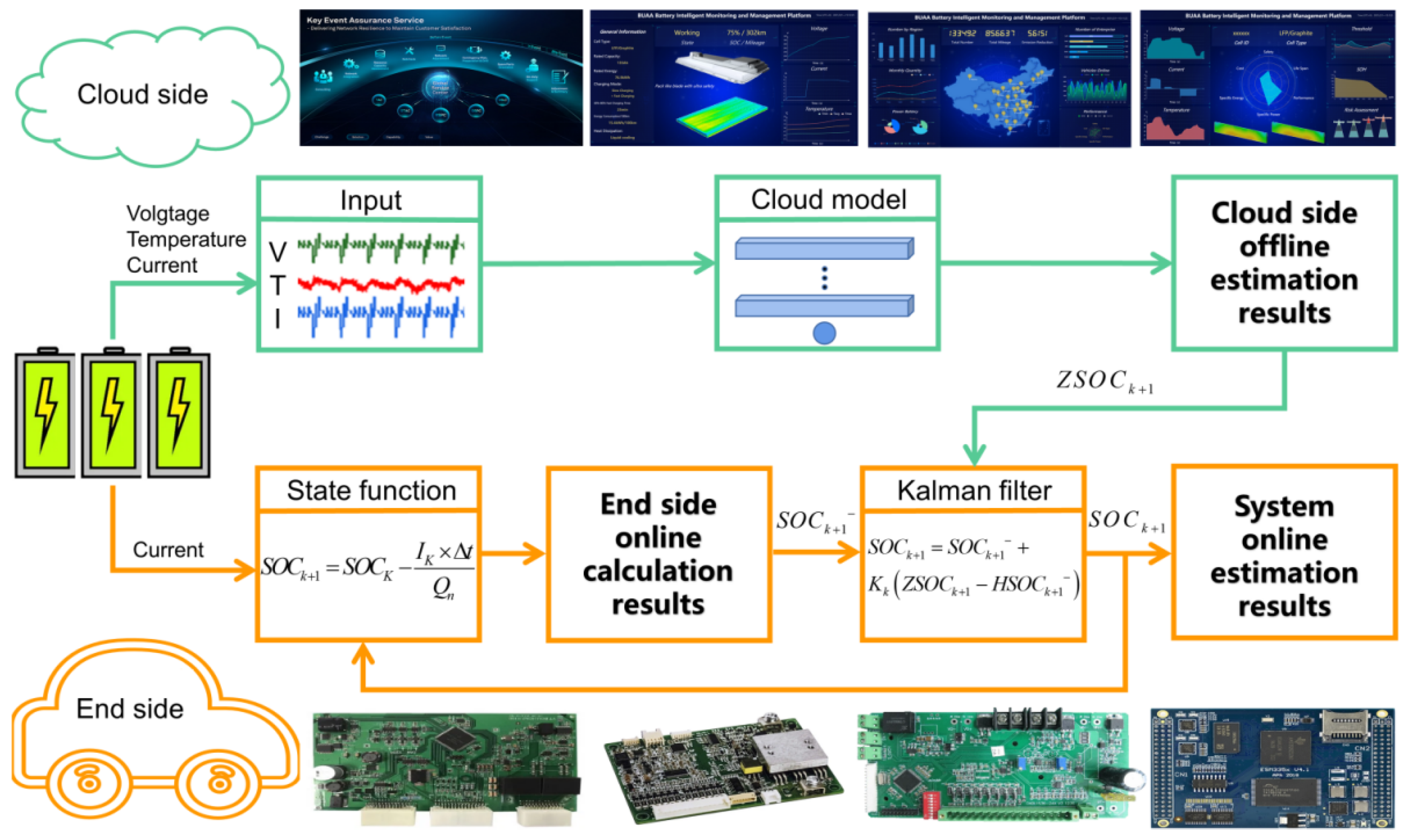
The framework of the proposed end-cloud collaboration SOC estimation system is represented in
Figure 3; the whole system is constructed based on the CHAIN framework [
35,
36]. On the cloud-side, the deep learning model estimates SOC, and the estimated results are regarded as the measured value. On the end-side, the state estimation is performed and the calculation results are regarded as the observed values, and then the collaborative algorithm is used to combine the calculation results of the end-side and the cloud-side, and update the result at each time step to obtain more accurate results. Specifically, in the training process, the deep learning model on the cloud-side uses a substantial amount of offline data from public datasets, enterprise databases, online data storage and other aspects to complete the training. During the estimation process, the voltage, current and temperature collected from the end-side are uploaded to the cloud-side. To estimate the battery SOC, and the cloud-side offline high-accuracy estimation results are obtained subsequently, the deep learning model on the cloud-side can estimate the SOC of the battery in the form of extrapolated estimation of historical data and the result will be used as the measured values of the Kalman’s filter, that is, the
in Expression (17) and the
in Expression (33) to update the end results. The coulomb counting method in end-side uses the current collected from the end-side to calculate the SOC, and the result will be used as the observed value of the Kalman’s filter, that is, the
in Expression (14) and the
in Expression (24). The Kalman’s filter is deployed on the end-side, and the real-time estimation results from the end-side and the estimation results from the cloud-side are received at the same time. Because the cloud-side is estimated by extrapolation, the cloud-side estimation results of the current time step have been obtained and transmitted in the previous time, so it can ensure that the transmission delay will not affect the real-time performance. The Kalman’s filter fuses the results from both sides to obtain the end-cloud collaborative high-accuracy and real-time estimation result, that is, the
in Expression (17) and the
in Expression (33), which is the final output of the entire end-cloud collaboration system. In practical applications, the whole end-cloud collaboration process can be realized through a cloud-based BMS [
37].
4. Result and Discussion
In this section, the accuracy and generalization of the CNN-LSTM network and the proposed end-cloud collaboration approach are evaluated firstly by estimating the SOC at different temperatures and different driving profiles. Secondly, the robustness of the proposed method is evaluated by manually setting different initial errors to estimate SOC under different temperatures. Meanwhile, the estimation results of KF and UKF as collaborative algorithms are compared in all experiments about the end-cloud collaboration approach.
4.1. Estimation Result of CNN-LSTM Network
In this subsection, the accuracy and generalization of the deep learning model on the cloud-side are evaluated at 0 °C, 25 °C and 40 °C, respectively.
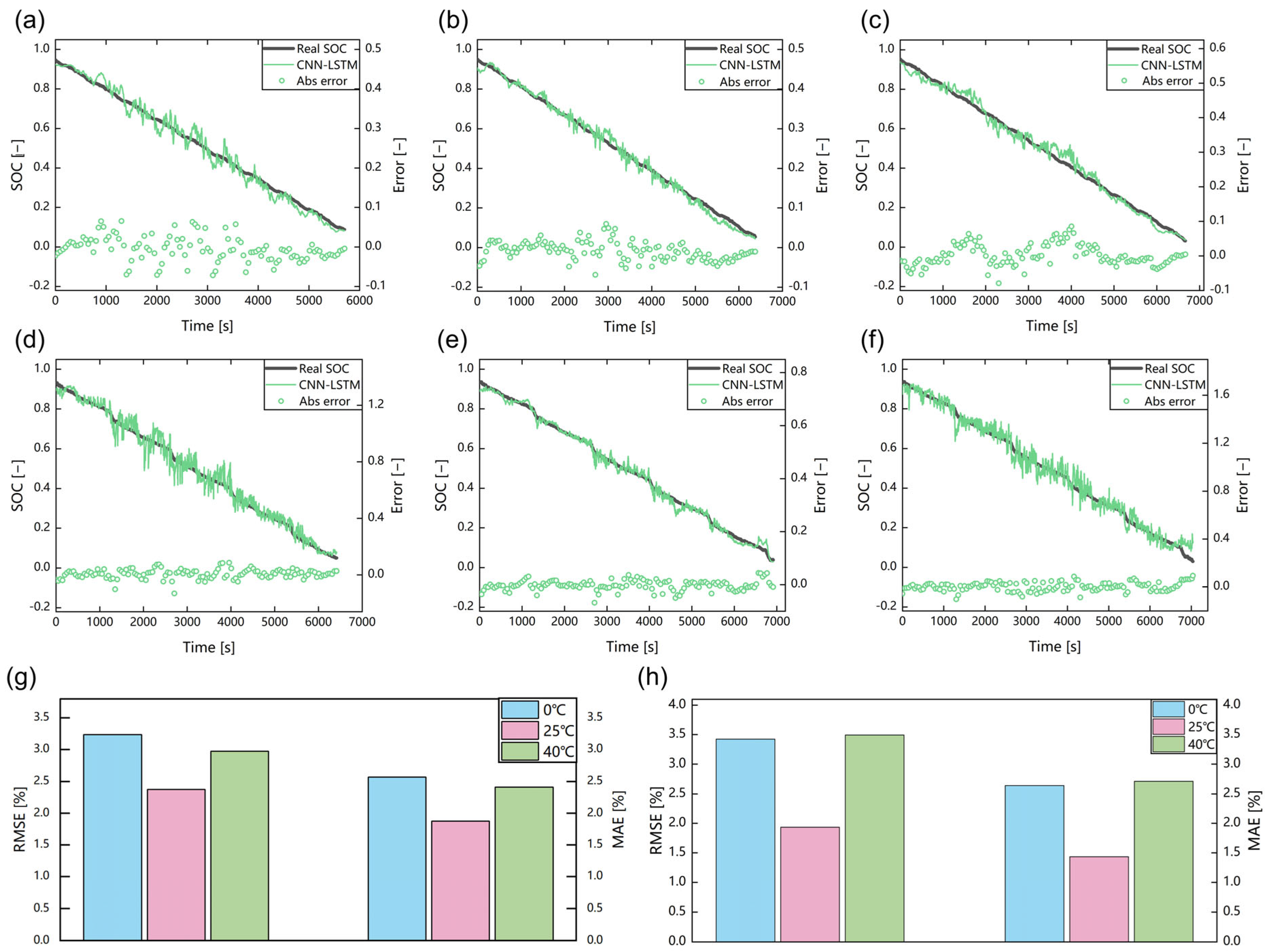
Figure 5a–f shows the estimation results and estimation errors of the CNN-LSTM network under US06 and FUDS profiles, respectively, while
Figure 5g,h show all estimation errors in the form of histograms. Each subgraph contains one dotted line and two solid lines. The black solid line illustrates the real SOC, the green solid line illustrates the estimation results of the CNN-LSTM network and the dotted line illustrates the estimation error of the CNN-LSTM network. The MAE and RMSE of the estimation results are about 2% and 3%, respectively. In particular, at 25 °C, the MAE and RMSE of the FUDS profile are 1.44% and 1.94%, respectively. However, the estimation results of the CNN-LSTM network fluctuate significantly, with a maximum estimation error is about 10%, and all appear in the middle regions, because the voltage characteristic curve having a plateau section in the middle region of SOC during battery discharge and cause the voltage change slope is so small that enlarge the deviation of the entire estimation results easily. Meanwhile, although the CNN-LSTM network has a strong generalization of the battery SOC estimation at different temperatures, the temperature will affect the estimation results. The error and fluctuation of the estimation results will increase at 0 °C and 40 °C. The maximum error is 8.57% at 25 °C under the US06 profile but will increase to 10% and 10.9%, respectively at 0 °C and 40 °C. At 25 °C under the FUDS profile, the maximum error is 7.8%, when the temperature is 0 °C and 40 °C, it will increase to 16.5% and 15.4%, respectively. The estimation error will also have a difference of about 1.5%. This is because the LiFeO
4 battery has a section of platform in the voltage characteristic curve and it will become flatter with the increase in temperature. Therefore, when the voltage measurement errors are the same, the estimation error of SOC will increase at high temperatures, while at low temperatures, with the increase in temperature, the internal resistance will increase rapidly and as a result, the polarization characteristic time at low temperature is very short, and the polarization voltage changes rapidly with temperature, increasing the estimation error.
4.2. Estimation Result of End-Cloud Collaboration Approach under Different Temperatures
In this subsection, the estimation accuracy and generalization of the proposed end-cloud collaboration approach are evaluated at 0 °C, 25 °C and 40 °C, respectively.
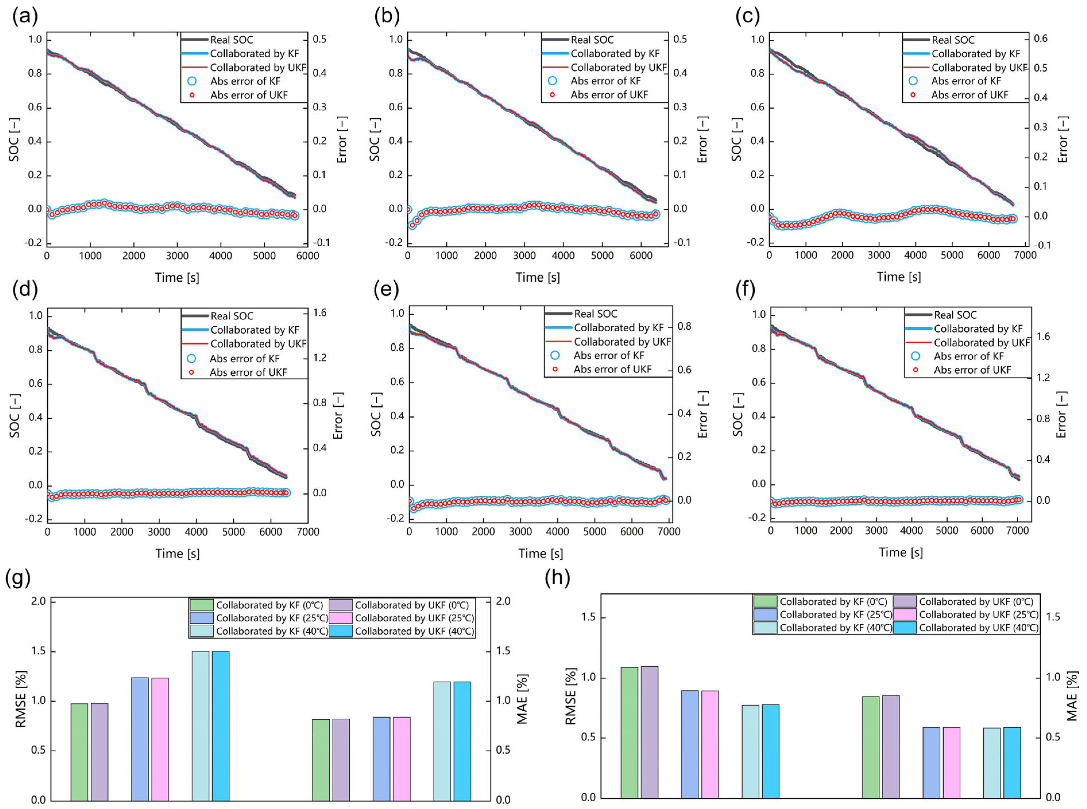
Figure 6a–f shows the estimation results and estimation errors of the end-cloud collaboration approach under US06 and FUDS profiles respectively, while
Figure 6g,h show all estimation errors in the form of histograms. Each subgraph contains two dotted lines and three solid lines. The black solid line represents the real SOC, the blue solid line represents the estimation result collaborated by KF, and the red solid line represents the estimation result collaborated by UKF. The dotted line represents the estimation error, and different colours correspond to the above solid lines one by one. The MAE and RMSE are all about 1%. In particular, at the FUDS profile under 40 °C, the MAE and RMSE are 0.58% and 0.77%, respectively. The accuracy of adopting KF and UKF as collaborative algorithms are almost the same, and the difference between MAE and RMSE is only about 0.01%. In most cases, the estimation accuracy of UKF is slightly lower than that of KF, but the difference is very small, which does not affect its application in practical applications. The difference between these two methods is little for the application is linear, but the approximate transformation will slightly reduce the accuracy when using UKF in linear problems.
Table 2 summarizes the estimation error of the end-cloud collaboration approach and the CNN-LSTM network. It can be seen that after the integration of the end-cloud collaboration system, the MAE and RMSE are reduced by about 1% and 2%, respectively compared with those of the single data-driven model, and the RMSE is reduced by 2.73% under the FUDS profile, particularly at 40 °C. Meanwhile, the maximum error of the end-cloud collaboration system has also been greatly reduced, and the maximum error is within 5%, which is more stable than the data-driven model. Furthermore, the estimation results of the single data-driven model will be affected for temperature, while the end-cloud collaboration approach is more stable at different temperatures, and the estimation error at room temperature is only 0.2% different from that at 0 °C and 40 °C. It can be seen that the end-cloud collaboration approach proposed in this work has high accuracy, and strong generalization and stability under different temperatures and driving cycles.
4.3. Estimation Result of End-Cloud Collaboration Approach under Different Initial SOC Errors
In practical applications, the challenging point in estimating the battery SOC is about the SOC estimation with the consideration of varying model parameters, which change with the temperature and aging state of the battery. On the end-side, the state function is built by the CCM, whose accuracy is highly dependent on the initial error, which will change at different temperatures and different aging process. On the cloud-side, the deep learning model can directly input the temperature as a feature into the network for training and prediction. Meanwhile, training data with different data distributions can be used to train battery SOC estimation models under different aging states to deal with the impact of different aging process. Thus, the estimated results of the model on the cloud-side can correct the influence of varying working environment. Therefore, to verify the ability of the proposed end-cloud collaboration approach to resist initial value dependence and converge, in this subsection, taking the FUDS profile as an example, SOC is estimated by manually setting the initial value error at different temperatures.
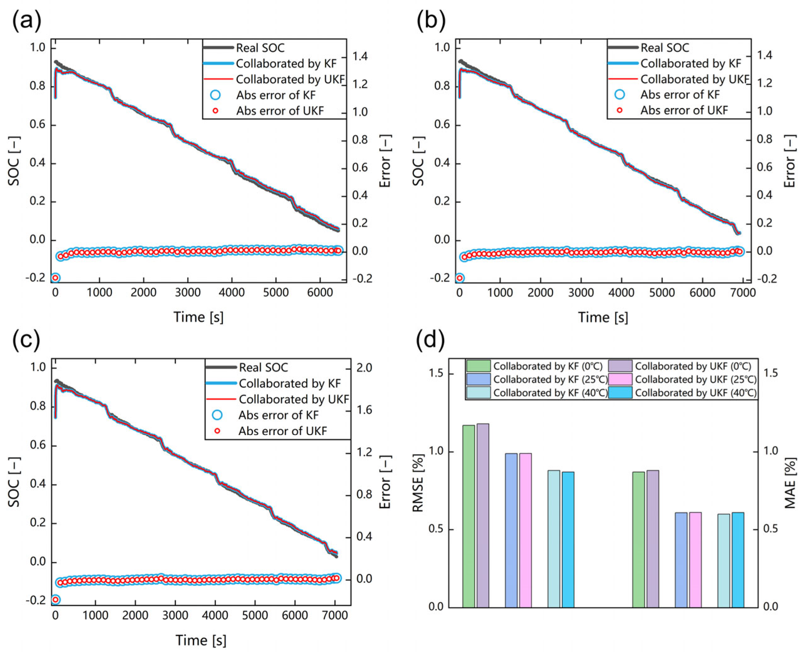
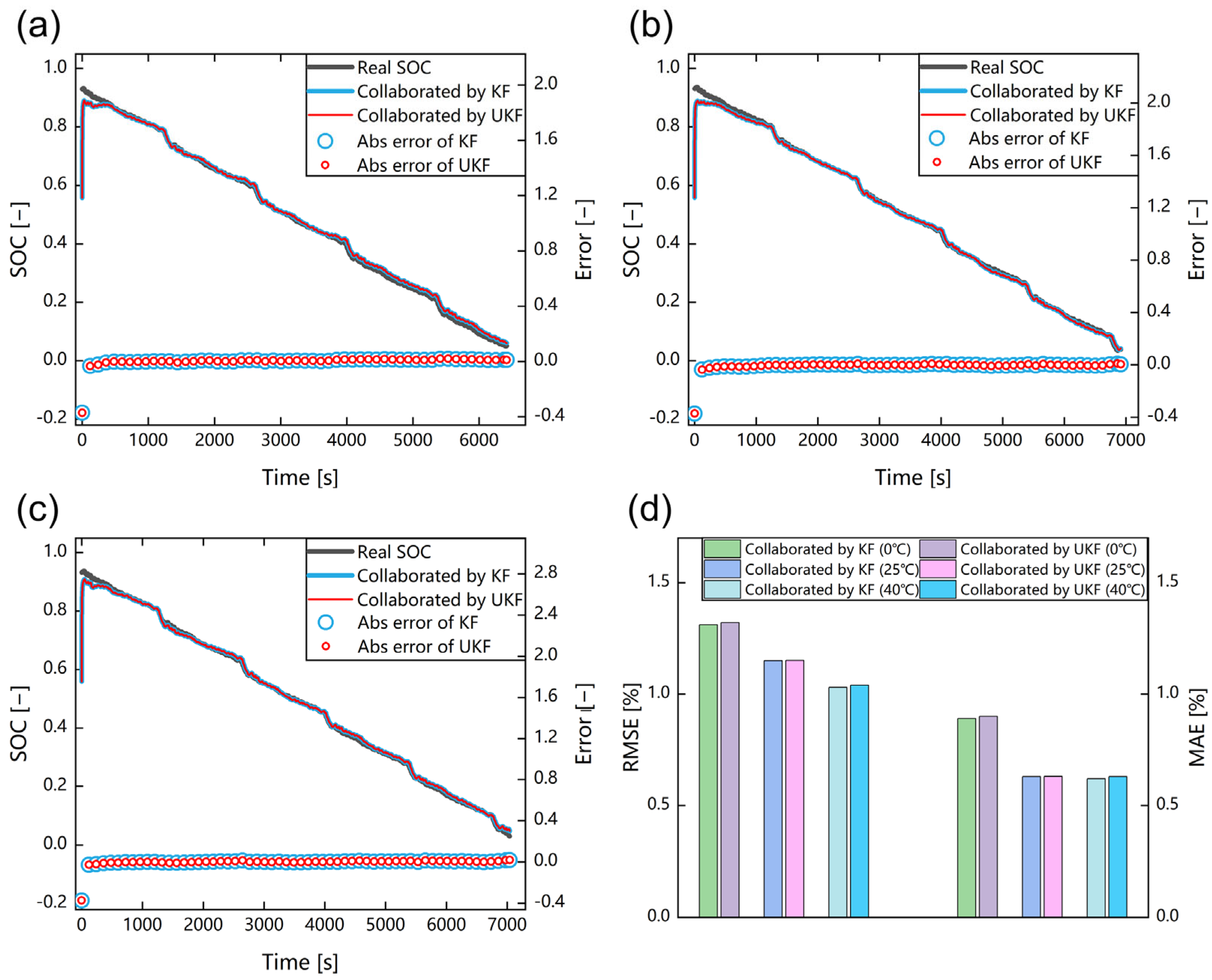
Figure 7a–c and
Figure 8a–c shows the estimation results and estimation errors of the end-cloud collaboration approach under the FUDS profile when the initial error is 20% and 40% of the true initial SOC, respectively.
Figure 7d and
Figure 8d show all estimation errors in the form of histograms. The lines and colours in each subgraph represent the same content as described in
Section 4.2. Specific error values are summarized in
Table 3.
Observe the overall deviation. When the initial SOC is 80% of the real initial SOC, the estimation results of the end-cloud collaboration system can still guarantee high accuracy. Compared with the case without initial value error, MAE and RMSE only increased by about 0.02% and 0.1%, respectively. Under the harsh case with the initial SOC is 60% of the real initial SOC, MAE and RMSE are only increased by about 0.04% and 0.3%, respectively. In particular, under the US06 profile at 40 °C, when the initial SOC was 0.8 and 0.6 of the real initial SOC, RMSE increased by only 0.05% and 0.16%, respectively.
Meanwhile, observing the initial error correction, it can be seen that under different initial errors, the proposed end-cloud collaboration approach can quickly complete the initial error correction, so that the estimation results can quickly converge to the level under true condition. When the initial SOC is 80% of the real initial SOC, the estimation result can converge to the accuracy equivalent to that under the condition of accurate initial SOC within 30 s, and the error can be converged within the maximum error of the condition of accurate initial SOC about 10 s. When the initial SOC is 60% of the real initial SOC, it can converge to the same accuracy as the condition of accurate initial SOC within 50 s, and the error can converge within the maximum error under the condition of accurate initial SOC about 20 s. The convergence speed of KF and UKF is almost the same.
In general, the proposed end-cloud collaboration approach can quickly complete the initial value error correction, thus avoiding the initial value dependence. Under different initial SOC conditions and different temperatures, it can achieve satisfactory accuracy, proving the robustness and stability of our method.
5. Conclusions
In this paper, the end-cloud collaboration approach is proposed to estimate the SOC for lithium-ion batteries online. The data-driven model is deployed on the cloud-side, and the coulomb counting method and Kalman’s filter are deployed on the end-side. The data-driven model is built with the CNN-LSTM network as the core. The potential features in the original data are extracted through CNN, and the time series features are captured from the information extracted from the CNN network through LSTM subsequently. During the experiment, the Bayesian optimization algorithm is used for the automatic optimization of hyperparameters, and the training process is completed through a substantial number of data provided by public data sets or databases offline. The voltage, current and temperature collected from end-side and uploaded to cloud, where such data is used for estimation. The state function constructed by the CCM is deployed at the end-side and is calculated online through the current monitored in real-time. The estimation results of data-driven model are regarded as measured values, and calculation results of the coulomb counting method are regarded as observed values. The Kalman’s filter simultaneously receives and fuses the calculation results from both the end side and cloud side, thus obtaining the final high-accuracy real-time output of the entire end-cloud collaboration system. Finally, the proposed end-cloud collaboration approach is evaluated under different temperatures and different initial errors with three dynamic driving profiles: DST, US06 and FUDS. The RMSE error is controlled less than 1.5%, and the maximum error is less than 5%, which indicates that the proposed end-cloud collaboration approach has high accuracy and strong robustness. By deploying a data-driven model on the cloud-side, deploying the coulomb counting method and Kalman’s filter on the end-side, and fusing the calculation results of the end-side and the cloud-side through Kalman filtering algorithm to obtain high-accuracy estimation results, the amount of calculation is transferred through end-cloud collaboration, thus realizing high-accuracy, real-time online estimation of battery SOC. The data-driven model on cloud-side is constructed based on the CNN-LSTM network, the potential features in the original data are extracted through CNN, and the long-term dependence on the time series is captured from the feature information extracted from CNN through LSTM subsequently and iterative training is conducted for many times, thus conducting effective dynamic modelling. In the dynamic working condition, the features contained in the measurable signal and the long-term dependence relationship with SOC can be well extracted. This approach has strong generalization for it is based on the data-driven and CCM, which eliminates the necessity to adjust model parameters promptly and consult tables to build appropriate OCV-SOC relationships at different temperatures. Meanwhile, this method has strong robustness which can automatically correct the initial value error to avoid initial value dependence and achieve satisfactory accuracy under different initial SOC conditions. It can complete the estimation task well under a variety of working conditions and initial errors and can be extended to batteries with different materials. This paper optimizes the estimation results and ensures real-time performance by arranging the models on the end-side and cloud-side respectively in the manner of end-cloud collaboration. Under the CHAIN framework, a high-accuracy and real-time SOC online estimation can be achieved through the proposed approach and this method can be extended to multi-state collaborative online estimation, making contributions to the development of the next generation of cloud-based BMS and end-cloud collaborative management system. In the future work, the impact of battery aging on SOC estimation will be considered through SOH and SOC collaborative estimation, and the proposed method will be further verified and optimized through real vehicle data verification and embedded development and can be expanded to application scenarios such as fault diagnosis and energy management.

 ,
, 


