An Extended Kalman Filter Design for State-of-Charge Estimation Based on Variational Approach

Abstract

State of charge (SOC) is a very important variable for using batteries safely and reliably. To improve the accuracy of SOC estimation, a novel variational extended Kalman filter (EKF) technique based on least square error method is herein provided by establishing a second-order equivalent circuit model for the battery. It was found that when SOC decreased, resistance polarization occurred in the electrochemical model, and the parameters in the equivalent RC model varied. To decrease the modeling error in the equivalent circuit model, the system parameters were identified online depending on the SOC’s estimated result. Through the SOC-estimation process, the variation theorem was introduced, which enabled the system parameters to track the real situations based on the output measured. The experiment results reveal the comparison of the SOC-estimation results of the variational EKF algorithm, the traditional EKF algorithm, the recursive least square (RLS) EKF algorithm, and the forgotten factor recursive least square (FFRLS) EKF algorithm based on different indices, including the mean square error (MSE) and the mean absolute error (MAE). The variational EKF algorithm provided in this paper has higher estimation accuracy and robustness than the traditional EKF, which verifies the superiority and effectiveness of the proposed method.

1. Introduction

In recent decades, with continuous climate change and extreme weather occurrences, environmental deterioration and the energy crisis have become some of the key problems to overcome [1]. To deal with such problems, strict policies for regulations of fuel consumption and CO₂ emission have been released throughout the world [2]. Therefore, developing sustainable clean energy is a global strategic policy. Moreover, the goal of carbon neutrality has become more and more popular as well [3,4]. Automotive manufacturers are focusing on developing electric vehicles due to their energy savings and pollution reduction for the environment, which offers great advantages and is a potential development trend compared to traditional cars [5,6]. As a conclusion, electric vehicles constitute a major development direction for automotive technology in the future [7,8]. To ensure that electric vehicles are utilized safely and reliably, a battery management system (BMS) is required for real-time battery-state monitoring. In the BMS, state of charge (SOC) is one of the core parameters to monitor [9]. Thus, obtaining an accurate real-time estimation value of the SOC is a significant goal for the future development of electric vehicles.

The SOC denotes the remaining capacity percentage of the battery, which is a key parameter in battery-state-estimation process. Many approaches have been studied by researchers to estimate the SOC, such as the open-circuit voltage (OCV) approach [10], the Coulomb counting approach [11], the model-based approach [12,13], and the data-driven approach [14]. The fundamental principle of the OCV approach depends on the nonlinear correlation between OCV and SOC, in which OCV is able to be established by a high-order function of SOC [10]. However, the drawback of this approach is that the lithium-ion battery must rest for a period of time before OCV measurements can be taken. Compared to the OCV approach, the Coulomb counting method is simple in implementation due to the convenient execution: Researchers only need to integrate the charging and discharging current of the battery [11]. Nevertheless, the measurement error is difficult to eliminate in the current integration process. The model-driven method is based on the establishment of the electrochemical model (EM) and the equivalent circuit model (ECM). It is capable of describing the internal principle of lithium-ion batteries based on the electrochemical characteristics in the EM [12]. For the ECM, the model is combined with the resistance, capacitance, and voltage source so that the dynamic process inside the lithium-ion batteries is simulated within different forms of the circuit [13]. The model-driven methods are based on basic theorems of the circuit, and the robustness is exhibited even with imprecise SOC initialization values and possible measurement noise. However, the model accuracy largely depends on the underlying battery model. The data-driven method is regarded as a “black box” mathematical model rather than a practical model [14]. Its results depend greatly on the quality of the input history data, whether the data are optimally trained, and whether the hyperparameters are suitably selected.

Considering the robustness of the model-driven methods, the Kalman filter (KF), which is known as the most common state-estimation technique, is utilized to estimate the optimal posterior SOC based on ECM [15,16]. Based on the KF framework, the extended Kalman filter (EKF) linearizes the evolution function and measurement function with first-order Taylor expansion to estimate the state for a nonlinear system [17]. Sun et al. proposed a new variational Bayesian (VB)-based adaptive extended Kalman filter (VBAEKF) for master–slave autonomous underwater vehicles (AUV) to deal with the unknown state noises and uncertain measurement noises encountered during underwater cooperative navigation [18]. Duan et al. utilized an improved EKF method with correlated entropy loss to improve the SOC-estimation accuracy for non-Gaussian cases [19]. Zhu et al. proposed a fractional-order adaptive extended Kalman filter (FO-AEKF) for SOC estimation, which can recursively update the noise covariance [20]. In reference [21], Paul et al. provided an optimized long short-term memory–weighted fading extended Kalman filtering (LSTM-WFEKF) model with the consideration of a temperature-adaptation model for SOC estimation, which introduced adaptive weighing and fading factors to correct and optimize the SOC value for different temperature variations under complex working conditions. Moreover, the unscented Kalman filter (UKF) based on unscented transform introduced sigma points that have same mean and variance as the state for nonlinear estimation [22]. With the help of radial basis function (RBF) networks and square-root UKF technique, Gholizade-Narm et al. provided a method for estimating the SOC of lithium-ion batteries [23]. When the nonlinear system is complex, the particle filter (PF) utilizes a large amount of particles to approximate the probability density function (PDF) of the state with the aim of estimating the updated state [24]. Accordingly, the UKF and PF have a more accurate estimation performance, but the implementation is more complex; the EKF is one of the simplest estimation techniques to be realized in many of the studies mentioned above, although the estimation is not as precise as other estimation methods in the Kalman framework. When the modelling parameters are accurate enough, the estimation performance of EKF and improved EKF algorithms are precise as well. Accordingly, the variation idea is proposed to solve the coupling problem of the state’s and system’s uncertainty for compensation. When the system is more certain, the estimated state is more accurate, and vice versa. The variation idea is employed in the variational Bayesian estimation, by which the state and the system parameters are estimated simultaneously by fixing a portion of the variables within the state and the system parameters [25]. As a consequence, the variation idea is an iteration process with heavy computational pressure to arrive at an accurate estimation performance within the Bayesian framework.

In this study, the model was established as a second-order RC model, and the parameters were identified based on the least square error technique. After the parameters were determined, the variational EKF algorithm was utilized, which optimizes the model accuracy and the estimation performance with simultaneous iterations. The main contribution of this study is the variational EKF algorithm in the SOC estimation for batteries. With the determination of the unique characteristics of the RC model in SOC estimation, the feasibility of the combination for the variation idea and the EKF algorithm is proposed. The variational EKF algorithm takes the model system parameters’ variations into consideration and estimates the SOC reasonably. The robustness and non-fragility of the algorithm is stronger than the traditional EKF algorithm due to the variational iteration.

The remaining sections of this paper are organized as following: Section 2 introduces the mathematical analysis for the architecture of the equivalent circuit model and the working principle of the traditional EKF algorithm in the SOC-estimation process. Section 3 proposes the flowchart for SOC estimation and provides the descriptions of the variational EKF algorithm. Section 4 describes the experimental validation of the study, including the experimental test platform, the experimental test procedure, the SOC-estimation results, and the performance comparison for the variational EKF, the traditional EKF, the RLS-EKF, the FFRLS-EKF algorithms based on the second-order RC models. Section 5 gives the conclusion of this paper.

2. Mathematical Analysis

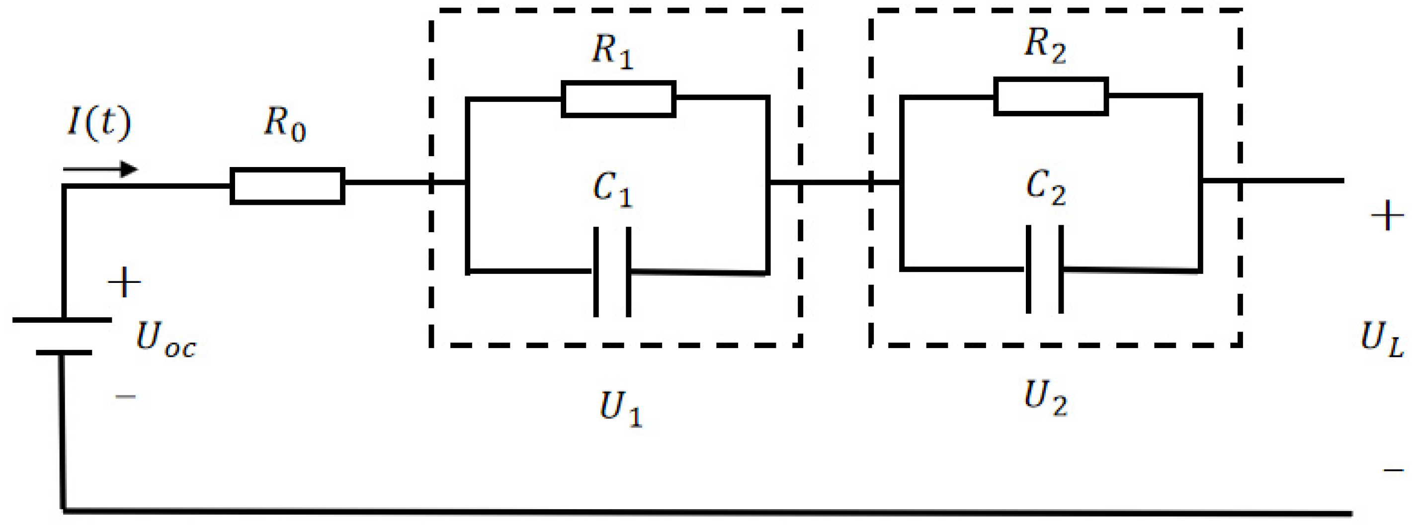
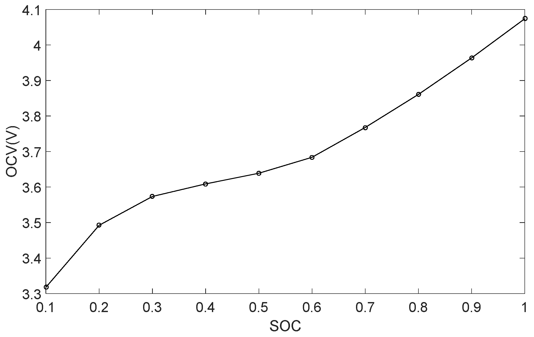
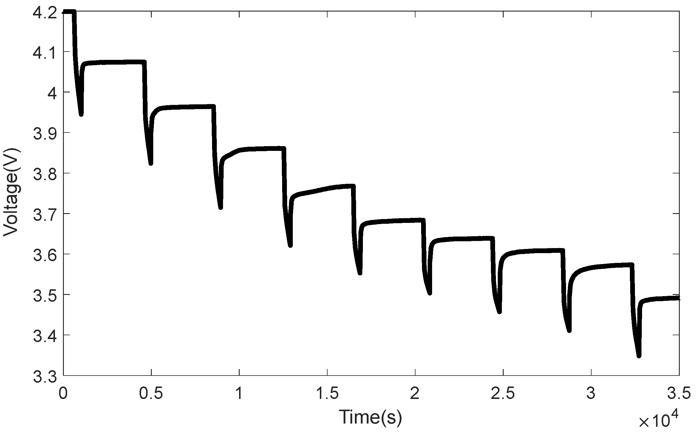
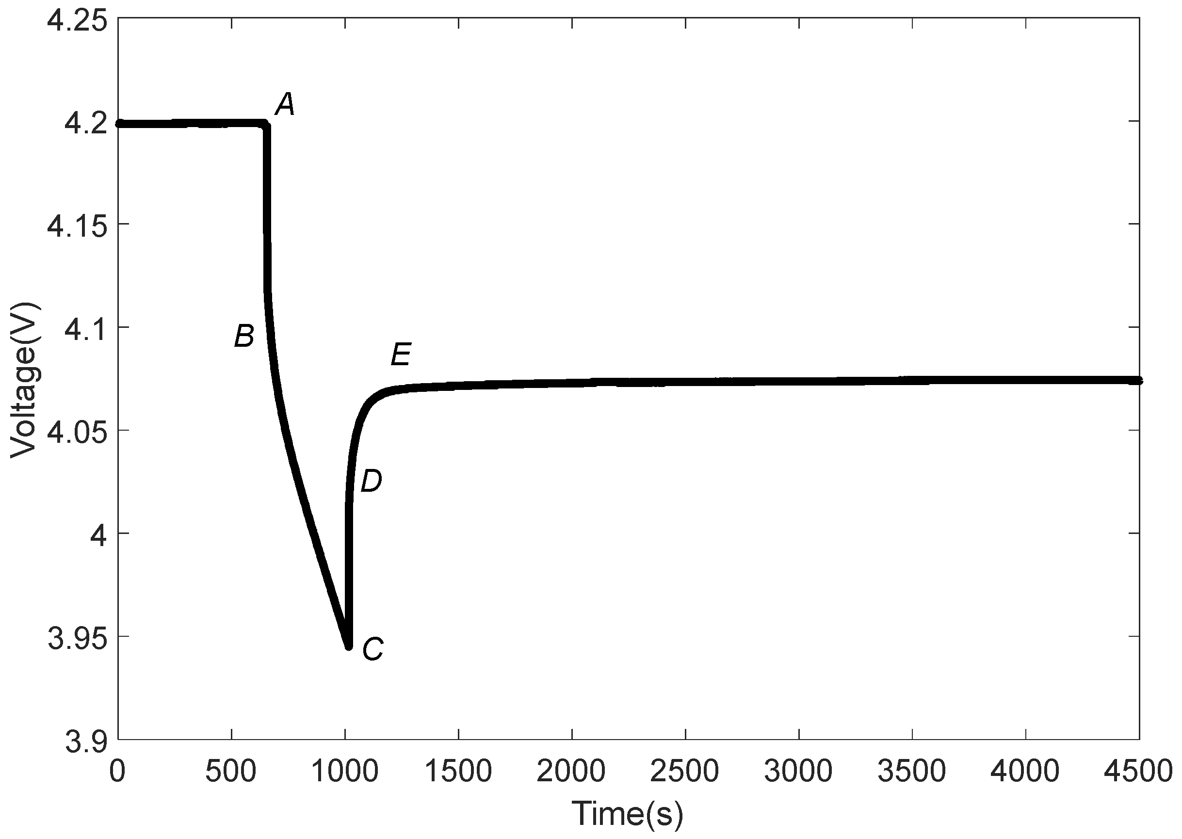
2.1. Battery Modelling

In general, the battery can be equivalently modeled as RC combinations. Considering that the battery-equivalent model is more accurate with more RC and results in heavier computational pressure, a suitable RC selection can balance the computational efficiency and estimation accuracy. In Figure 1, the second-order RC model as utilized is shown [26].

In Figure 1, the battery state of charge (SOC) is defined as the ratio of the residual capacity to the nominal capacity. In practical applications, the most commonly used method to estimate SOC is the Coulomb counting technique, which accumulates the charge transferred in or out of the battery to determine the change of the SOC. Thus, the initial SOC must be precise for SOC estimation in this method. In Equation (1), the SOC at time $t$ is denoted as follows [27]:

$$SOC(t)=SOC(t_0)-\frac{1}{Q_0}{\displaystyle \underset{t_0}{\overset{t}{\int }}\eta I(t)dt}$$

(1)

where $SOC(t_0)$ is the SOC value at time $t_0$, $Q_0$ is the nominal capacity, $\eta$ is the Coulomb efficiency, and $I(t)$ denotes the time-varying current. Then, with the help of Kirchhoff’s law of the circuit, the second-order RC model can be obtained by the following Equations (2)–(4):

$${\dot{U}}_1(t)=-\frac{1}{R_1{C}_1}{U}_1(t)+\frac{1}{C_1}I(t)$$

(2)

$${\dot{U}}_2(t)=-\frac{1}{R_2{C}_2}{U}_2(t)+\frac{1}{C_2}I(t)$$

(3)

$$U_L(t)=U_{OC}(t)-U_1(t)-U_2(t)-R_{0}I(t)$$

(4)

In Equations (2) and (3), $U_1(t)$ and $U_2(t)$ denote the terminal voltages of two RC circuit loops, respectively. $U_{OC}(t)$ is the measured OCV, which establishes the relationship with SOC by the polynomial of the OCV-SOC fitting curve, as in Figure 2.

According to the differential Equations (2) and (3), $U_1(t)$ and $U_2(t)$ are solved. Then, the discrete state space based on Equations (2)–(4) is proposed as the state space model system (5).

$$\{\begin{array}{c}x(k+1)=Ax(k)+Bu(k)+w(k)\\ y(k)=Cx(k)+Du(k)+U_{OC}(k)+v(k)\end{array}$$

(5)

In system (5), the state variable $x(k)={\left[\begin{array}{ccc}SOC(k)& U_1(k)& U_2(k)\end{array}\right]}^T$, the input $u(k)=I(k)$, and the outputs $y(k)=U_L(k)$. $w(k)$ and $v(k)$ are the Gaussian system noise, and measurement noise with zero mean and the variance are $Q$ and $R$, respectively. $U_{OC}(k)$ is the discrete form of $U_{OC}(t)$. The state space parameters are given as follows:

$$\begin{array}{c}A=\left[\begin{array}{ccc}1& 0& 0\\ 0& e^{-\frac{\Delta t}{R_1{C}_1}}& 0\\ 0& 0& e^{-\frac{\Delta t}{R_2{C}_2}}\end{array}\right], B={\left[\begin{array}{ccc}-\frac{\eta }{Q_0}& R_1\left(1-e^{-\frac{\Delta t}{R_1{C}_1}}\right)& R_2\left(1-e^{-\frac{\Delta t}{R_2{C}_2}}\right)\end{array}\right]}^T,\hfill \\ C=\left[\begin{array}{ccc}0& -1& -1\end{array}\right]\mathrm{and}D=R_0\hfill \end{array}$$

where $\Delta t=1$ is the sampling rate of the discrete system.

In the system (5), the parameters are written as the function of the second-order RC model parameters $R_1$, $C_1$, $R_2$, $C_2$, and $R_0$ given in Figure 1. These parameters are identified based on the hybrid pulse power characteristic (HPPC) test of the battery. The time-varying battery discharge voltage in the HPPC test is given in Figure 3 [26]. In the HPPC test procedure, the voltage of the battery is 4.2 V in the beginning, which means the battery SOC is 100% and at full charge. During the HPPC process, the battery is discharged by a 1 C current for 6 min at 25 °C in the discharging step; then, the battery is preserved for 60 min in the preserving step. Therefore, the time range of the measured voltage curve of the battery is 66 min. The discharging and preserving step in the HPPC test process needs to be repeated ten times. The battery SOC is reduced by 10% after each repetition. In the end, the battery SOC is reduced to 0, which means the battery runs out of power.

To explain in detail, Figure 4 provides a pulse of the HPPC test in Figure 3. In Figure 4 [26], time A is the beginning of discharging, and time C is the end of discharging. In the figure, the voltage decreases sharply from time A to time B and the voltage decreasing speed significantly slows down from time B to time C. Simultaneously, it can be found that the voltage decreases at time A and increases at time C; time C to time E denotes the battery preserving time after discharging with zero current $I(0)=0$. The voltage increases rapidly from time C to time D and voltage increasing speed significantly slows down from time D to time E. Consequently, the internal resistance $R_0$ can be determined by the voltage variation as follows:

$$R_0=\frac{\left(U_A-U_B\right)+\left(U_D-U_C\right)}{2I}$$

(6)

where $U_A$, $U_B$, $U_C$, and $U_D$ are the voltages at times A, B, C, and D in Figure 4, respectively. The dynamic characteristics of $U_1(t)$ and $U_2(t)$ of the battery are given as follows:

$$U_1(t)=U_1(0)e^{-\frac{t}{R_1{C}_1}}+I{R}_1\left(1-e^{-\frac{t}{R_1{C}_1}}\right)$$

(7)

$$U_2(t)=U_2(0)e^{-\frac{t}{R_2{C}_2}}+I{R}_2\left(1-e^{-\frac{t}{R_2{C}_2}}\right)$$

(8)

Then, the output based on zero input $I(t)=0$ can be written by substituting Equations (7) and (8) in the state space model (5) through the stabilization process in Figure 4 from time C to time D as follows:

$$\begin{array}{cc}\hfill U_L(t)& =U_{OC}-U_1(t)-U_2(t)\hfill \\ & =U_{OC}-U_1(0)e^{-\frac{t}{R_1{C}_1}}-U_2(0)e^{-\frac{t}{R_2{C}_2}}\hfill \end{array}$$

(9)

The curve fitting tool in MATLAB2022a software was utilized to perform custom equation fitting of the polarization voltage based on the following equation:

$$f(t)=a_0-a_1{e}^{-b_{1}t}-a_2{e}^{-b_{2}t}$$

(10)

Referring to Equations (8) and (9), the parameters can be obtained as follows:

$$U_{OC}=a_0,U_1(0)=a_1,R_1{C}_1=\frac{1}{b_1},U_2(0)=a_2\mathrm{and}{R}_2{C}_2=\frac{1}{b_2}$$

(11)

Before time A in Figure 4, the battery has been preserved enough times so that the polarization and concentration effect is nearly zero. From time A to time C in Figure 4, the battery is discharging with invariable current. With the substitution $t=0$ into Equations (7) and (8), it is easy to find $U_1(0)=I{R}_1$ and $U_2(0)=I{R}_2$. Then, the parameters in the second-order RC model can be identified as follows:

$$R_1=\frac{a_1}{I},C_1=\frac{I}{a_1{b}_1},R_2=\frac{a_2}{I}\mathrm{and}{C}_2=\frac{I}{a_2{b}_2}$$

(12)

To determine the relationship between $U_{OC}(t)$ and SOC shown in Figure 2, which are obtained by the measurement of the battery discharge voltage in the HPPC test from Figure 3, the MATLAB curve fitting tool was utilized, and its fitting polynomial is given as follows:

$$\begin{array}{cc}\hfill U_{OC}& =12.6667SO{C}^6-38.7423SO{C}^5+40.1910SO{C}^4\hfill \\ \hfill & -12.2887SO{C}^3-4.1345SO{C}^2+3.3490SOC+3.0330\hfill \end{array}$$

(13)

From Figure 3, it is obvious that the parameters in the second-order RC model are variables with different SOCs based on Equations (6) and (12). Similarly, the fitting polynomial for the second-order RC model parameters can be derived as follows:

$$\begin{array}{cc}\hfill R_0& =5.5499SO{C}^6-24.4678SO{C}^5+38.0322SO{C}^4\hfill \\ \hfill & -25.2196SO{C}^3+5.6661SO{C}^2+0.9635SOC-0.3488\hfill \end{array}$$

(14)

$$\begin{array}{cc}\hfill R_1& =24.1999SO{C}^6-87.3629SO{C}^5+125.7313SO{C}^4\hfill \\ \hfill & -91.9119SO{C}^3+35.8142SO{C}^2-7.0041SOC+0.5513\hfill \end{array}$$

(15)

$$\begin{array}{cc}\hfill C_1& =7.1098\times {10}^{5}SO{C}^6-2.6085\times {10}^{6}SO{C}^5+3.7925\times {10}^{6}SO{C}^4\hfill \\ \hfill & -2.7592\times {10}^{6}SO{C}^3+1.0443\times {10}^{6}SO{C}^2-1.9416\times {10}^{5}SOC+1.5661\times {10}^4\hfill \end{array}$$

(16)

$$\begin{array}{cc}\hfill R_2& =-26.6129SO{C}^6+104.0744SO{C}^5-158.7476SO{C}^4\hfill \\ \hfill & +118.6184SO{C}^3-43.8665SO{C}^2+7.0261SOC-0.2359\hfill \end{array}$$

(17)

$$\begin{array}{cc}\hfill C_2& =-5.6107\times {10}^{5}SO{C}^6+1.5432\times {10}^{6}SO{C}^5-1.5337\times {10}^{6}SO{C}^4\hfill \\ \hfill & +7.0519\times {10}^{5}SO{C}^3-2.0315\times {10}^{5}SO{C}^2+5.4359\times {10}^{4}SOC+640.8538\hfill \end{array}$$

(18)

According to Equations (13)–(18), it is obvious that the parameters $A$, $B$, $C$, and $D$ in the state space model (5) vary depending on the state variable SOC, which results in the deficiency of the traditional recursive state-estimation algorithms.

2.2. Extended Kalman Filter

Previously, in Section 2.1, the system parameters in the state space model (5) were shown varying depending on the state variable SOC. In this way, it is clear that the system (5) is nonlinear, and the estimation error of the traditional Kalman filter is unneglectable because the Kalman filter only determines the best expectation for the estimation based on the linear system and white Gaussian noise [15]. When it comes to nonlinear systems, the Kalman filter is unable to provide the optimal estimation result.

In this way, the extended Kalman filter (EKF) is proposed to deal with such estimation problems in a nonlinear system, which is an improvement of the traditional Kalman filter algorithm. The EKF algorithm for a discrete system is given as follows:

$$\{\begin{array}{c}x(k+1)=f\left(x(k),u(k)\right)+w(k)\\ y(k)=g\left(x(k),u(k)\right)+v(k)\end{array}$$

(19)

where $f\left(x(k),u(k)\right)$ and $g\left(x(k),u(k)\right)$ are continuously differentiable nonlinear functions in Equation (19).

The EKF introduces the first-order Taylor expansion for the nonlinearities of $x(k)$, which is given as follows:

$$\{\begin{array}{c}x(k+1)=\tilde{A}\left(x(k|k)\right)x(k)+\tilde{B}\left(x(k|k)\right)u(k)+w(k)\\ y(k)=\tilde{C}\left(x(k|k)\right)x(k)+\tilde{D}\left(x(k|k)\right)u(k)+v(k)\end{array}$$

(20)

where $x\left(k|k\right)$ is the posterior estimation of state $x$ at time $k$, and the system parameters are differentiated as $\tilde{A}\left(x\left(k|k\right)\right)={\frac{df}{dx}|}_{x=x\left(k|k\right)}$, $\tilde{B}\left(x\left(k|k\right)\right)={\frac{df}{du}|}_{x=x\left(k|k\right)}$, $\tilde{C}\left(x\left(k|k\right)\right)={\frac{dg}{dx}|}_{x=x\left(k|k\right)}$, and $\tilde{D}\left(x\left(k|k\right)\right)={\frac{dg}{du}|}_{x=x\left(k|k\right)}$.

Then, the process of the recursive Traditional EKF algorithm is provided as Algorithm 1 in the following:

Algorithm 1 Traditional EKF Algorithm

$\mathrm{Step}1:\mathrm{Initializing}\mathrm{the}\mathrm{initial}\mathrm{state}x(0)$$\mathrm{and}\mathrm{the}\mathrm{variance}P(0)$.

Step 2: Predicting the one step prior state prediction and variance.

$x\left(k+1|k\right)=f\left(x(k|k),u(k)\right)$

$P\left(k+1|k\right)=\tilde{A}\left(k|k\right)P\left(k|k\right)\tilde{A}\left(k|k\right)+Q$

Step 3: Computing the filter gain.

$\begin{array}{cc}\hfill K\left(k+1\right)& =P\left(k+1|k\right){\tilde{C}}^T\left(x\left(k+1|k\right)\right)\hfill \\ \hfill & \times [\tilde{C}\left(x\left(k+1|k\right)\right)P\left(k+1|k\right){\tilde{C}\left(x\left(k+1|k\right)\right)+R]}^{-1}\hfill \end{array}$

Step 4: Calculating the one step posterior state estimation and variance

$x\left(k+1|k+1\right)=x\left(k+1|k\right)+K\left(k+1\right)\left[y\left(k\right)-g\left(x(k),u(k)\right)\right]$

$P\left(k+1|k+1\right)=[I-K\left(k+1\right)\tilde{C}\left(x\left(k+1|k\right)\right)]P\left(k+1|k\right)$

Step 5: Repeating Step 2 to Step 4.

The traditional EKF algorithm may cause divergence in the filtering process mainly due to the unreasonable mathematical model. The linearized parameters are derived based on the Jacobian of the nonlinear function. In this way, it is clear that the model only satisfies first-order accuracy, which means that once the system’s nonlinearity come to the higher order, the approximated linearized system is unable to follow the original nonlinear system well. Therefore, when the estimation result of the EKF algorithm is inaccurate, and the approximated linearized system is unable to approximate the original nonlinear system, especially with strong nonlinearity.

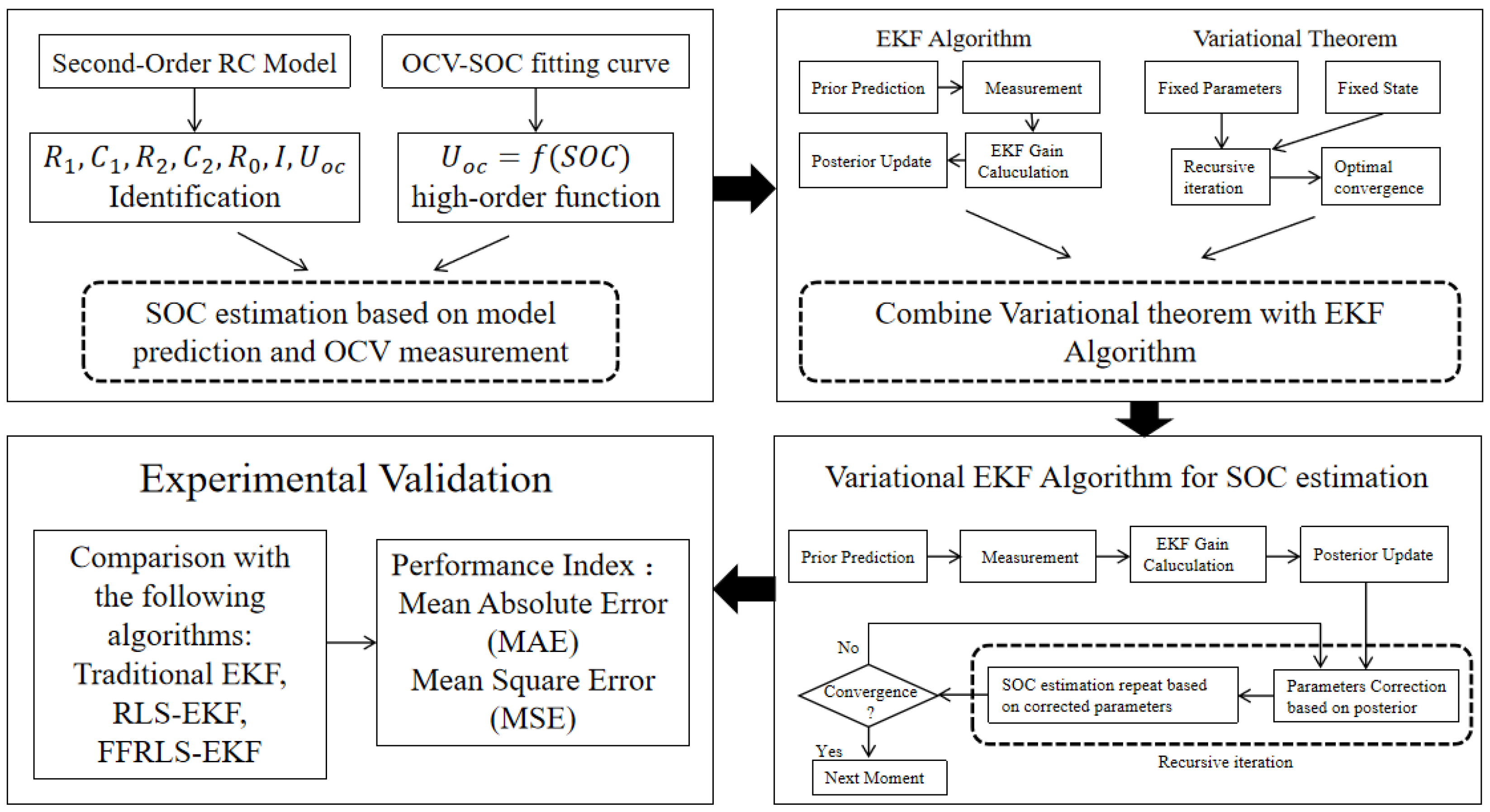
3. SOC Estimation Based on Variational Extended Kalman Filter Algorithm

To compensate the drawbacks of EKF as mentioned above, the idea of parameter variation was introduced. With the introduction of such an idea, the traditional EKF was improved by recursive iteration for the linearized parameters depending on the posterior estimation of SOC, with estimation of the SOC depending on the parameters obtained in the previous iteration.

In the variational EKF algorithm, the posterior estimation result of the SOC is obtained based on the EKF algorithm depending on the system parameters determined by the estimated SOC in the previous iteration. Then, the parameters are determined based on the updated estimation result of the SOC obtained by Equations (14)–(18). It is clear that the approximated linearized system is able to arrive at the estimation result, which is close to the original nonlinear function based on the accurate estimated SOC. With this confirmation, the system parameters and the SOC estimation result are closer to the true value in every iteration simultaneously. The variational EKF algorithm is given as Algorithm 2 in the following.

Algorithm 2 Variational EKF Algorithm

Step 1: Initializing the initial state $x(0)$ and the variance $P(0)$.

Step 2: Figuring out the one step prior to state prediction $x\left(k+1|k\right)$ and variance $P\left(k+1|k\right)$, the filter gain $K\left(k+1\right)$, and the posterior state estimation $x\left(k+1|k+1\right)$ and variance $P\left(k+1|k+1\right)$ based on traditional EKF algorithm mentioned in Algorithm 1.

Step 3: Computing the system parameters $\tilde{A}\left(x\left(k+1|k+1\right)\right)$, $\tilde{B}\left(x\left(k+1|k+1\right)\right)$, $\tilde{C}\left(x\left(k+1|k+1\right)\right)$, $\tilde{D}\left(x\left(k+1|k+1\right)\right)$ based on Equations (13)–(18) with the introduction of the posterior state estimation $x\left(k+1|k+1\right)$.

Step 4: Comparing the difference between the posterior state estimated by step 2 and step 3; if the difference is small enough, then go to next step; if the difference is large, then send the posterior state estimation in step 3 to step 2, and repeat step 3;

Step 5: Replacing moment $k$ by moment $k+1$ and repeating step 2–4.

With the variational EKF algorithm proposed, the most important highlight is the variation cycle in each time moment. The variation cycle recursively estimates the posterior state based on traditional EKF and improves the linearized system parameters depending on the estimated posterior state. With more accurate linearized system parameters, the estimation result is closer to the true value, and with an estimation result closer to the true value, the linearized system parameters provide a more accurate estimation result. Therefore, the variation cycle is able to help the traditional EKF algorithm to estimate the posterior state more accurately. For better understanding, a flow chart of this process is provided in Figure 5 to show the logical order and algorithm flow.

Furthermore, the most common drawback of traditional EKF is the heavy computational pressure for the Jacobian matrix computation. As mentioned in [27], the number of floating operations (flops) required to implement the EKF equations from step 2 to step 4 in Algorithm 1 at each recursion is given approximately as follows:

$$Coun{t}_{EKF}=3n_x^3+\left(3n_y+\frac{5}{2}\right)n_x^2+3\left(n_y^2+n_y\right)n_x+\frac{2}{3}{n}_y^3+\frac{3}{2}{n}_y^2+\frac{5}{6}{n}_y$$

(21)

From Equation (21), it can be inferred that when the state dimension $n_x$ is very large, direct implementation of the EKF is not possible because of the cubic term $3n_x^3$ due to the computation of the Jacobian matrix, the prior variance $P\left(k|k-1\right)$, and the inverse matrix in Kalman gain. Nevertheless, when it comes to the SOC estimation, the Jacobian matrix computation is not as heavy as other EKF circumstance because all the differentials in the linearized system parameters are only for the component SOC in the state vector and have no relationship with other components in the state vector. Simultaneously, the parameter in the linearized system is a diagonal matrix obtained by the Kirchhoff’s law circuit, which indicates that the computational pressure of solving the inverse matrix for the Kalman gain in the EKF algorithm is not as heavy as traditional EKF applications but is approximately of $n_x^2$ order of magnitude. In this way, the computation pressure is tolerable, and the introduction of the variation idea is possible.

In Section 4, the experiment’s validation results are shown to prove the reliability and superiority of the variational EKF algorithm. The traditional EKF, the RLS-EKF, and the FFRLS-EKF are compared for the SOC-estimation process based on five batteries of the same type.

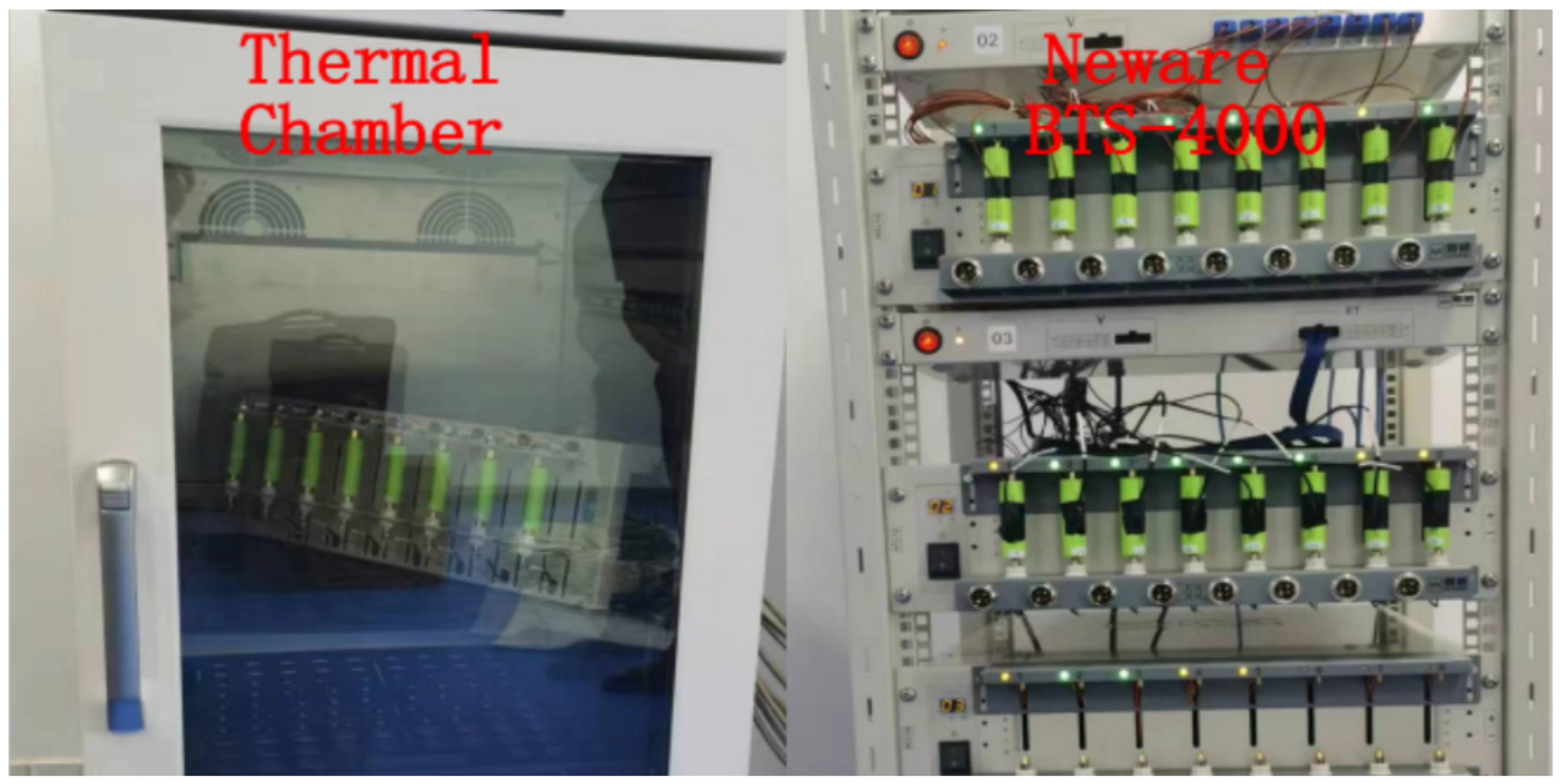
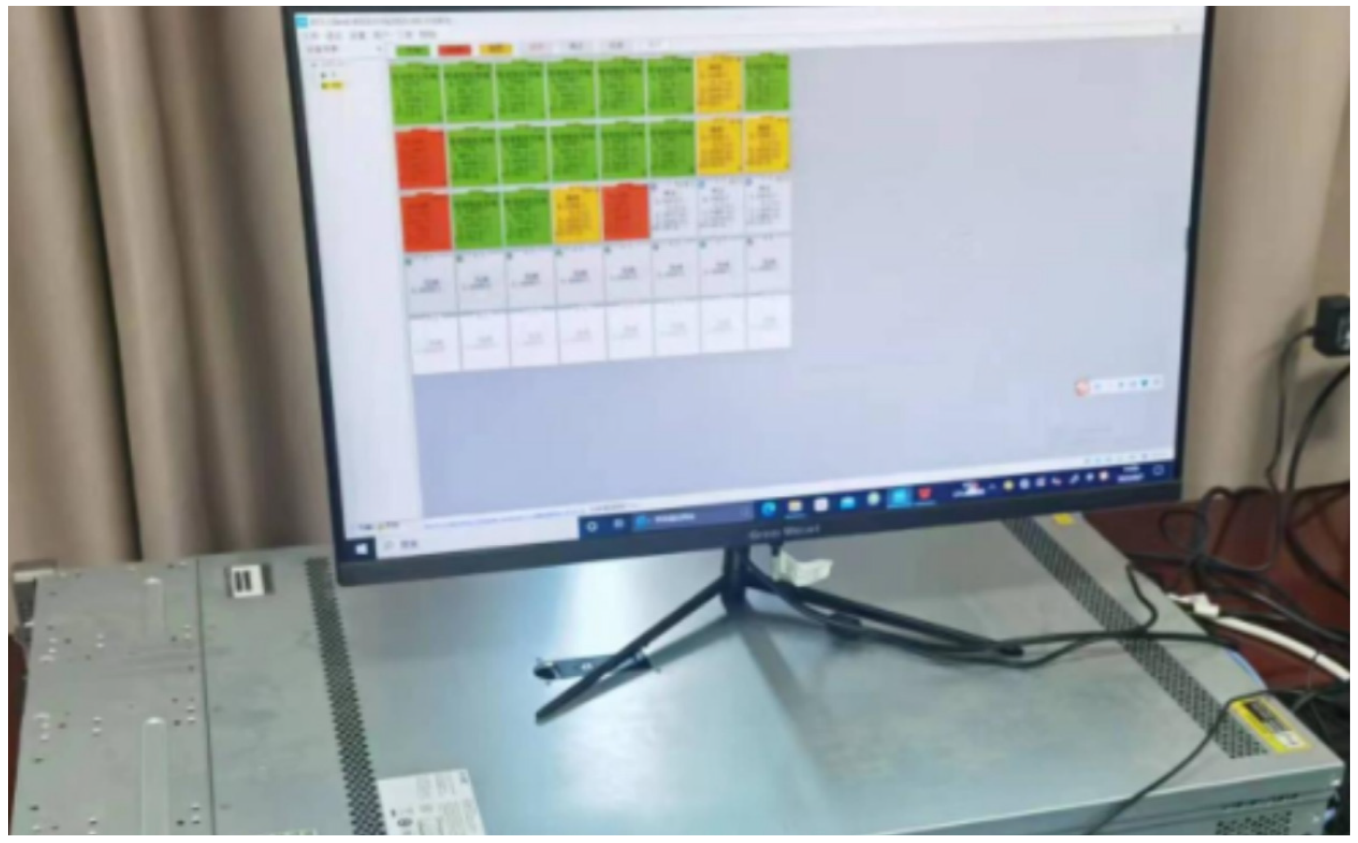
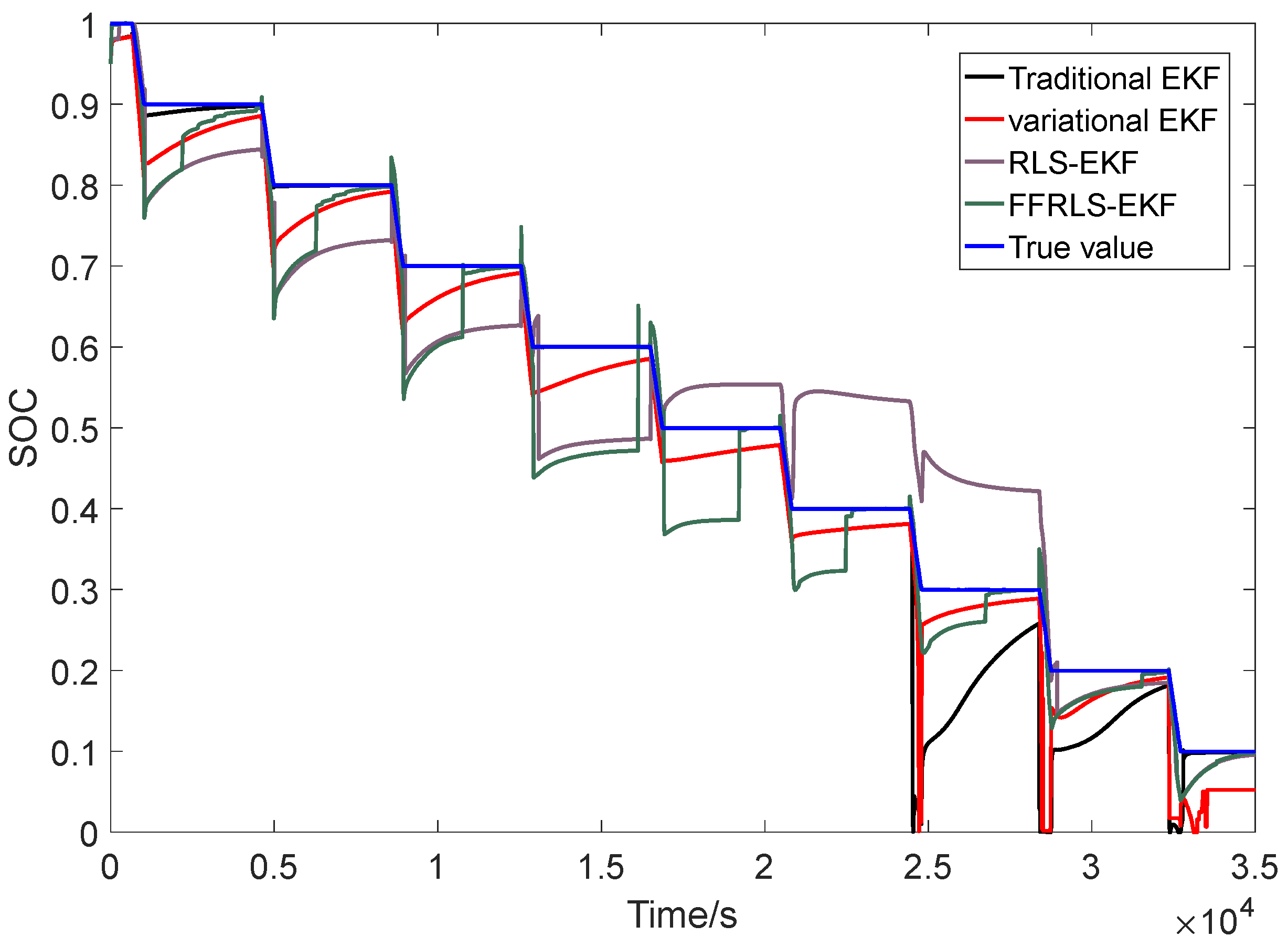
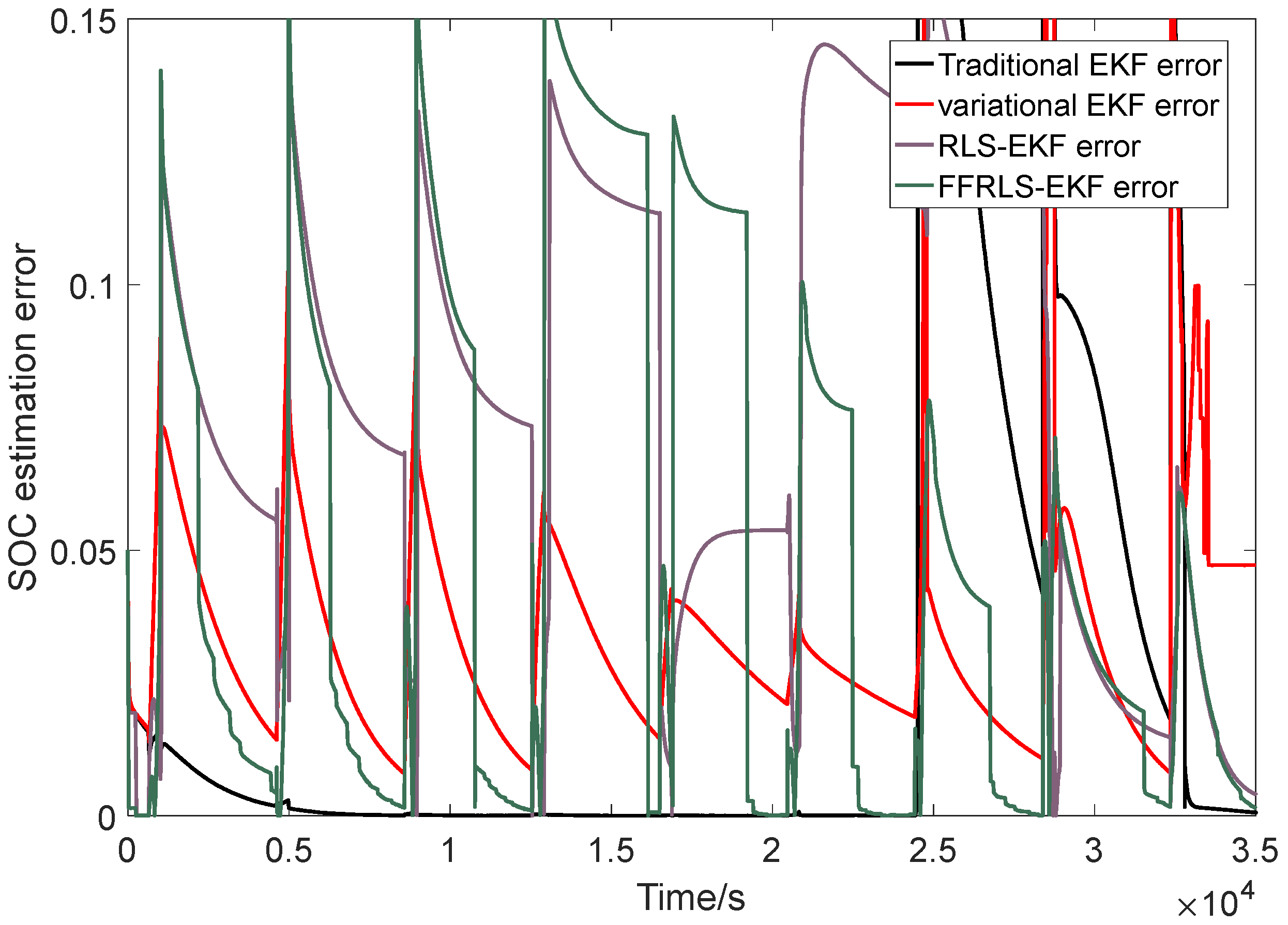
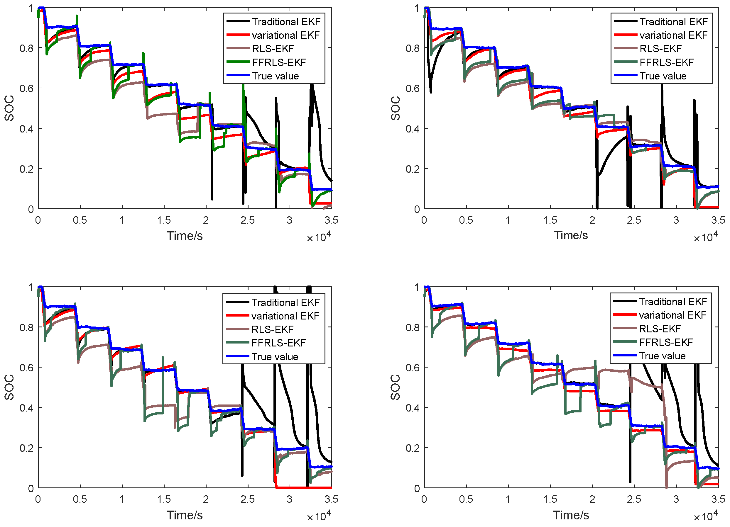
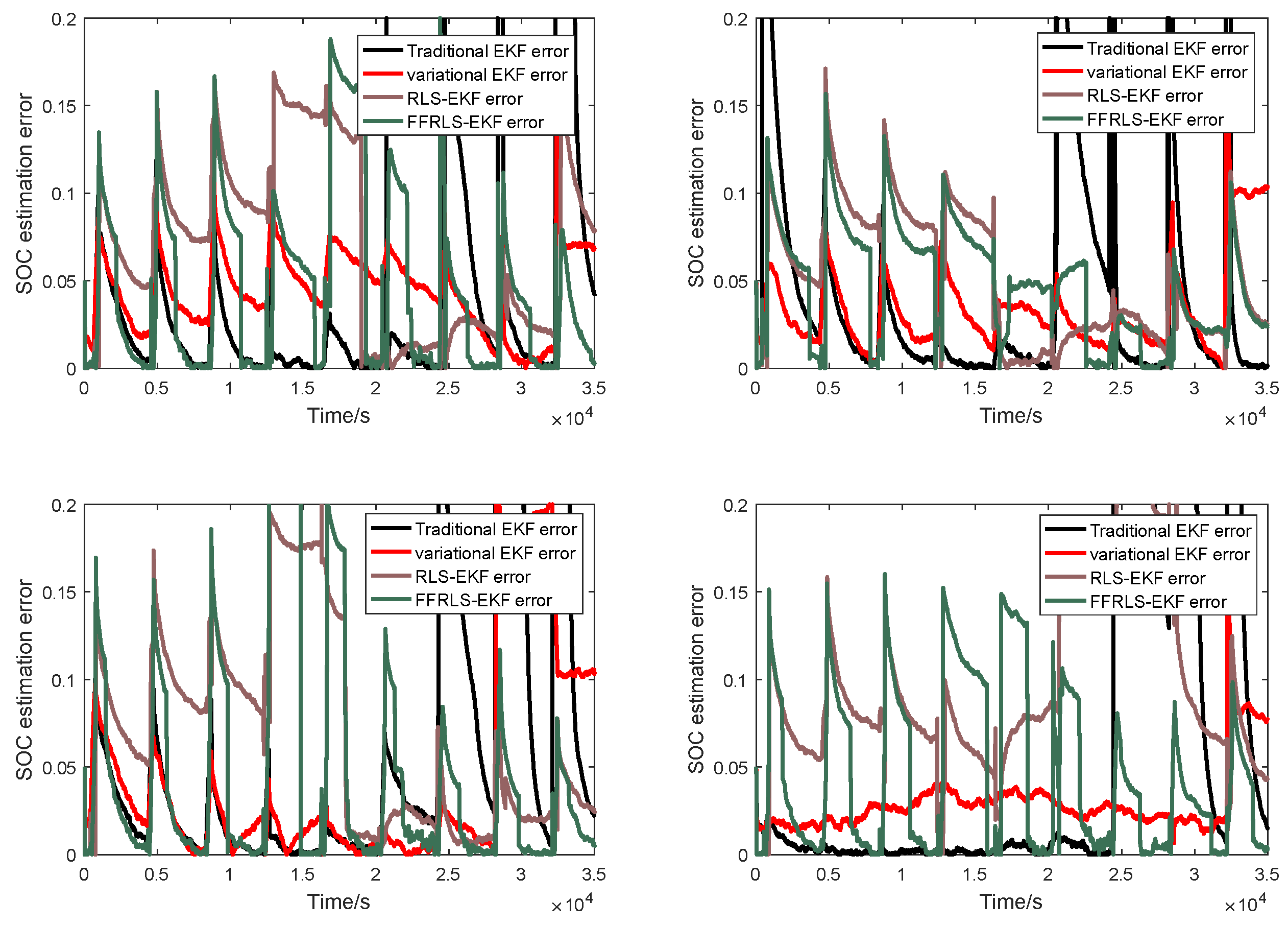
4. Experimental Validation

The effectiveness of the variational EKF algorithm in SOC estimation was revealed through the comparative experiments explained in this section. This study utilized the 18650 lithium-ion battery test with a rated capacity of 2.5 Ah as the research object, and the experimental platform was utilized to set the working conditions by the charge–discharge instrument in Figure 6 and battery manage system in Figure 7. As shown in Figure 6, the battery measurement system includes a battery testing system (BTS) and a thermal chamber from Neware manufacturer (Shenzhen, China). The type of BTS is Neware BTS-4000, which is carried out battery aging experiments at different charging rates. The type of the thermal chamber is Neware MHW-200, which is used to control the battery temperatures. Figure 7 shows that the battery aging data are measured by a battery management system in the Industrial Personal Computer (IPC). The green, red, and orange color blocks in the figure denote the charging, discharging, and temporary waiting of batteries. In the charging and discharging process, the hybrid pulse power characteristic (HPPC) test of the battery was performed to obtain the discharge data and was conducted with a NEWARE BTS-4000 in a 5 V 20 A working condition and at 25 °C working temperature. The detailed parameters of the 18650 battery are given in

Table 1. The parameters of the 18650 battery.

Battery Model	LR1865SZ
Nominal capacity	2.5 Ah
Minimum capacity	2.4 Ah
Charging voltage	4.2 V
Nominal voltage	3.0 V
Maximum charging current	1 C (2.4 A)
Maximum discharging current	1 C (2.4 A)

.

Five batteries of the same type were tested in the experiment. The tested batteries have different RC model parameters; nevertheless, the estimation result based on variational EKF is always better than that based on traditional EKF, the RLS-EKF, and the FFRLS-EKF, which shows the robustness of the variational EKF algorithm compared to the other methods. In the RLS-EKF algorithm, the RLS technique is able to derive the real-time characteristics by recursively updating the system parameters [28]. Compared to the RLS-EKF, the FFRLS-EKF introduces the forgotten factor to decrease the early date weights, which makes the updated parameters of the system more reasonable. The initialization of the tested batteries is given as follows. The true value of SOC at the beginning is 100%, and the initial parameters of the variational EKF and the comparison EKF algorithms are $x\left(0\right)=95\%$ and $P(0)={10}^{-4}$. The variance of the system noise and the measurement noise is $Q={10}^{-4}$ and $R={10}^{-4}$, respectively. In the experiment, the SOC is estimated based on the RC model and the measured OCV in the HPPC test according to the OCV-SOC fitting curve obtained in Figure 2.

The experimental results for battery No. 1 are provided in Figure 8 and Figure 9. The estimation comparison of the traditional EKF algorithm, the variational EKF algorithm, the RLS-EKF, and the FFRLS-EKF is given in Figure 8. From this figure, it is obvious that the variational EKF estimation result is closer to the true value of SOC compared to the other EKF estimation results. With the introduction of the variation technique, the linearized system parameters are approximated to the nonlinear system parameters. Therefore, the estimation result is accurate, demonstrating the algorithm’s ability to determine the true SOC value well even when a signal mutation or measurement error exists. The estimation error comparison between the EKF algorithms is given in Figure 8. Similarly, the experimental results for batteries No. 2 through No. 5 are given in Figure 10 and Figure 11. Obviously, the estimation result comparison and the estimation error have a similar tendency with battery No. 1, and the variational EKF performs better than the other EKF algorithms. The reason is that the RC model parameters are determined depending on the estimated SOC but not the true value, and the estimation result gives an inaccurate performance when the initialization is far from the true SOC or when sudden extreme cases occur in the estimation process. In these circumstances, the other EKF algorithms’ performance is not as good as that of the variational EKF due to the parameters’ correction from the variation part. The detailed experimental testing data are shown in

Table 2. The Experimental Testing Data of Batteries.

Battery No.	Initial Voltage (V)	Discharge Current (mA)	Discharge Capacity (mAh)	Discharge Energy (mWh)
No. 1	4.1238	2352.4	2337.614	9083.854
No. 2	4.1319	2379.7	2362.726	9173.627
No. 3	4.1282	2367.3	2361.838	9174.183
No. 4	4.1378	2328.8	2317.366	9001.016
No. 5	4.1307	2346.2	2336.890	9065.465

. The SOC estimation based on variational EKF algorithm are other EKF algorithms depends on these test data.

To make the experimental results more persuasive, the estimation results were tested based on simulations with different random noise sequences with the help of a Monte Carlo (MC) simulation algorithm. Each battery was simulated 100 times for the random noise in different sequences. In this way, the estimation error of the variational EKF was proven to still be significantly less than that of the other EKF algorithms. To demonstrate the superiority of the variational EKF algorithm, the mean absolute error (MAE) and the mean square error (MSE) of several EKF algorithms for batteries No. 1 through No. 5 during 100 simulations are given in

Table 3. Performance index comparison between the variational EKF and other EKF algorithms.

Battery No.	Algorithm	MAE	MSE
No. 1	Variational EKF	0.0357	0.0021
	Traditional EKF	0.0262	0.0037
	RLS-EKF	0.0779	0.0081
	FFRLS-EKF	0.0482	0.0047
No. 2	Variational EKF	0.0448	0.0025
	Traditional EKF	0.0425	0.0097
	RLS-EKF	0.0702	0.0075
	FFRLS-EKF	0.0455	0.0047
No. 3	Variational EKF	0.0343	0.0019
	Traditional EKF	0.0421	0.0062
	RLS-EKF	0.0505	0.0038
	FFRLS-EKF	0.0467	0.0032
No. 4	Variational EKF	0.0453	0.0057
	Traditional EKF	0.0720	0.0237
	RLS-EKF	0.0683	0.0079
	FFRLS-EKF	0.0455	0.0062
No. 5	Variational EKF	0.0298	0.0012
	Traditional EKF	0.0733	0.0263
	RLS-EKF	0.0990	0.0128
	FFRLS-EKF	0.0454	0.0042

to prove the effectiveness and the reliability of the variational EKF algorithm.

In detail, it is easily observed that the estimation error of all the EKF algorithms has a spike at the end of every discharge step. This phenomenon occurs mainly owing to the mismatch between the model prediction and OCV measurement results. If the model is accurate enough, the estimation results of EKF algorithm will be accurate as well. All the EKF algorithms gradually converge to the true value of SOC in the preserving step. At the high-SOC part, the traditional EKF algorithm performs better than the variational EKF, which is shown in Table 3. However, when it comes to low-SOC part, the performance of the traditional EKF algorithm decreases sharply. The reason is that the modeling error is unable to be ignored during the RC model parameter identification process. When the model parameters are not accurate at low-SOC part, the EKF is unable to determine an accurate posterior estimation result. Nevertheless, the variational EKF algorithm has better performance at the low-SOC part, which results from the recursive parameter and estimation result iteration by the variational theorem. In Figure 8 and Figure 10, the variational EKF algorithm performs much better than other EKF algorithms. The performance indices provided in Table 3 show that the variational EKF has the lowest MSE for all the batteries and the lowest MAE for batteries No. 3 through No. 5. The traditional EKF algorithm has a lower MAE than the variational EKF algorithm in batteries No. 1 and No. 2. This result depends on the RC model accuracy by which the traditional EKF is able to track the SOC well at the high-SOC part. At the low-SOC part, the model’s accuracy reduction is not significant enough, and the SOC-estimation error is averaged by the good performance at the high-SOC part. The MSE magnifies the estimation error comparison, especially at the low-SOC part. Therefore, even though the traditional EKF algorithm has a lower MAE in some cases, the variational EKF algorithm is robust for most battery cases, and the superiority and the effectiveness are extremely obvious.

5. Conclusions

In this paper, a variational EKF algorithm is provided to estimate the SOC of lithium-ion batteries. Firstly, the input battery datasets were modeled as a second-order RC model based on the least square error curve fitting technique. Secondly, the SOC estimation was obtained by the variational EKF and other EKF algorithms based on the second-order RC model, respectively. With the introduction of the variational theorem, the estimation result of the improved EKF algorithm was more accurate than that of the other EKF algorithms. The result provides low noise and good error-correction ability. The variational EKF algorithm estimated the SOC for battery No. 1 with the overall best MAE, with MSE values of 0.0355 and 0.0019 under the HPPC working condition, respectively, which manifests the superiority and reliability of the variational EKF algorithm. However, the initialization value of the variational EKF algorithm still affects the estimation accuracy. Therefore, in future work, we will focus on reducing the effectiveness of the imprecise initialization value.

References

1. Kampa, M.; Castanas, E. Human health effects of air pollution. Environ. Pollut. 2008, 151, 362–367. [Google Scholar] [CrossRef]
2. Ge, S.; Xu, L.; Liu, H.; Fang, J. Low-carbon benefit analysis on DG penetration distribution system. J. Mod. Power Syst. Clean Energy 2015, 3, 139–148. [Google Scholar] [CrossRef]
3. Biswas, P. Adapting SUV AWD powertrain to P0/P2/P4 hybrid EV architecture: Integrative packaging and capability study. In Proceedings of the IEEE Transportation Electrification Conference, Pune, India, 13–15 December 2017. [Google Scholar]
4. Sun, F.C. Green Energy and Intelligent Transportation-promoting green and intelligent mobility. Green Energy Intell. Transp. 2022, 1, 100017. [Google Scholar] [CrossRef]
5. Lane, B.; Shaffer, B.; Samuelsen, S. A comparison of alternative vehicle fueling infrastructure scenarios. Appl. Energy 2020, 259, 114128. [Google Scholar] [CrossRef]
6. Hannan, M.A.; Lipu, M.S.H.; Hussain, A.; Mohamed, A. A review of lithium-ion battery state of charge estimation and management system in electric vehicle applications: Challenges and recommendations. Renew. Sustain. Energy Rev. 2017, 78, 834–854. [Google Scholar] [CrossRef]
7. Kiaee, M.; Cruden, A.; Sharkh, S. Estimation of cost savings from participation of electric vehicles in vehicle to grid (V2G) schemes. J. Mod. Power Syst. Clean Energy 2015, 3, 249–258. [Google Scholar] [CrossRef]
8. He, H.W.; Sun, F.C.; Wang, Z.P.; Lin, C.; Zhang, C.; Xiong, R.; Deng, J.; Zhu, X.; Xie, P.; Zhang, S.; et al. China’s battery electric vehicles lead the world: Achievements in technology system architecture and technological breakthroughs. Green Energy Intell. Transp. 2022, 1, 100020. [Google Scholar] [CrossRef]
9. Xiong, R.; Kim, J.; Shen, W.X.; Lv, C.; Li, H.; Zhu, X.; Zhao, W.; Gao, B.; Guo, H.; Zhang, C.; et al. Key technologies for electric vehicles. Green Energy Intell. Transp. 2022, 1, 100041. [Google Scholar] [CrossRef]
10. Chen, Y.; Yang, G.; Liu, X.; He, Z. A time-efficient and accurate open circuit voltage estimation method for lithium-ion batteries. Energies 2019, 12, 1803. [Google Scholar] [CrossRef]
11. Movassagh, K.; Raihan, A.; Balasingam, B.; Pattipati, K. A critical look at coulomb counting approach for state of charge estimation in batteries. Energies 2021, 14, 4074. [Google Scholar] [CrossRef]
12. Shao, Y.; Liu, H.; Shao, X.D.; Sang, L.; Chen, Z.T. An all coupled electrochemical-mechanical model for all-solid-state Li-ion batteries considering the effect of contact area loss and compressive pressure. Energy 2022, 239, 121929. [Google Scholar] [CrossRef]
13. Nejad, S.; Gladwin, D.T.; Stone, D.A. A systematic review of lumped-parameter equivalent circuit models for real-time estimation of lithium-ion battery states. J. Power Sources 2016, 316, 183–196. [Google Scholar] [CrossRef]
14. Dong, G.; Yang, F.; Wei, Z.; Wei, J.; Tsui, K.L. Data-driven battery health prognosis using adaptive Brownian motion model. IEEE Trans. Ind. Inform. 2019, 16, 4736–4746. [Google Scholar] [CrossRef]
15. Meng, J.H.; Ricco, M.; Luo, G.Z.; Swierczynski, M.; Stroe, D.; Stroe, A.; Teodorescu, R. An overview and comparison of online implementable SOC estimation methods for lithium-ion battery. IEEE Trans. Ind. Appl. 2017, 54, 1583–1591. [Google Scholar] [CrossRef]
16. Xiong, R.; Sun, F.C.; He, H.W. Data-driven State-of-Charge estimator for electric vehicles battery using robust extended Kalman filter. Int. J. Automot. Technol. 2014, 15, 89–96. [Google Scholar] [CrossRef]
17. Sun, D.; Yu, X.; Wang, C.; Zhang, C.; Bhagat, R. State of charge estimation for lithium-ion battery based on an Intelligent Adaptive Extended Kalman Filter with improved noise estimator. Energy 2021, 214, 119025. [Google Scholar] [CrossRef]
18. Sun, C.J.; Zhang, Y.G.; Wang, G.Q.; Gao, W. A New Variational Bayesian Adaptive Extended Kalman Filter for Cooperative Navigation. Sensors 2018, 18, 2538. [Google Scholar] [CrossRef]
19. Duan, J.; Wang, P.; Ma, W.; Qiu, X.; Fang, S. State of charge estimation of lithium battery based on improved correntropy extended Kalman filter. Energies 2020, 13, 4197. [Google Scholar] [CrossRef]
20. Zhu, Q.; Xu, M.; Liu, W.; Zheng, M.Q. A state of charge estimation method for lithium-ion batteries based on fractional order adaptive extended kalman filter. Energy 2019, 187, 115880. [Google Scholar] [CrossRef]
21. Takyi-Aninakwa, P.; Wang, S.; Zhang, H.; Yang, X.Y.; Fernandez, C. An optimized long short-term memory-weighted fading extended Kalman filtering model with wide temperature adaptation for the state of charge estimation of lithium-ion batteries. Appl. Energy 2022, 326, 120043. [Google Scholar] [CrossRef]
22. He, W.; Williard, N.; Chen, C.; Pecht, M. State of charge estimation for Li-ion batteries using neural network modeling and unscented Kalman filter-based error cancellation. Int. J. Electr. Power Energy Syst. 2014, 62, 783–791. [Google Scholar] [CrossRef]
23. Gholizade-Narm, H.; Charkhgard, M. Lithium-ion battery state of charge estimation based on square-root unscented Kalman filter. IET Power Electron. 2013, 6, 1833–1841. [Google Scholar] [CrossRef]
24. Wang, S.; Fernandez, C.; Fan, Y.C.; Feng, J.Q.; Yu, C.M.; Huang, K.F.; Xie, W. A novel safety assurance method based on the compound equivalent modeling and iterate reduce particle-adaptive Kalman filtering for the unmanned aerial vehicle lithium ion batteries. Energy Sci. Eng. 2020, 8, 1484–1500. [Google Scholar] [CrossRef]
25. Yun, Z.; Qin, W.; Shi, W. State of charge estimation of lithium-ion battery under time-varying noise based on Variational Bayesian Estimation Methods. J. Energy Storage 2022, 52, 104916. [Google Scholar] [CrossRef]
26. Liu, R.; Zhang, C. An Active Balancing Method Based on SOC and Capacitance for Lithium-Ion Batteries in Electric Vehicles. Front. Energy Res. 2021, 9, 773838. [Google Scholar] [CrossRef]
27. Ait-El-Fquih, B.; Hoteit, I. Fast Kalman-like filtering for large-dimensional linear and Gaussian state-space models. IEEE Trans. Signal Process. 2015, 63, 5853–5867. [Google Scholar] [CrossRef]
28. Ren, B.; Xie, C.; Sun, X.D.; Zhang, Q.; Yan, D. Parameter identification of a lithium-ion battery based on the improved recursive least square algorithm. IET Power Electron. 2020, 13, 2531–2537. [Google Scholar] [CrossRef]
Figure 1. The Second-Order RC Model [26].
Batteries 09 00583 g001
Figure 2. OCV-SOC fitting curve.
Batteries 09 00583 g002
Figure 3. Battery discharge voltage in the HPPC test [26].
Batteries 09 00583 g003
Figure 4. Battery discharge voltage in a pulse of the HPPC test [26].
Batteries 09 00583 g004
Figure 5. The EKF.
Batteries 09 00583 g005
Figure 6. The charge–discharge instrument for lithium-ion battery test.
Batteries 09 00583 g006
Figure 7. The IPC of the charge–discharge instrument.
Batteries 09 00583 g007
Figure 8. Estimation result comparison between the variational EKF and other EKF algorithms.
Batteries 09 00583 g008
Figure 9. Estimation error comparison between the variational EKF and other EKF algorithms.
Batteries 09 00583 g009
Figure 10. Estimation result comparison for batteries No. 2 through No. 5.
Batteries 09 00583 g010
Figure 11. Estimation error comparison for batteries No. 2 through No. 5.
Batteries 09 00583 g011