Article

Cloud-Based Optimization of a Battery Model Parameter Identification Algorithm for Battery State-of-Health Estimation in Electric Vehicles

1
Dipartimento di Ingegneria dell’Informazione, University of Pisa, Via Caruso 16, 56122 Pisa, Italy
2
TECH, Advanced Connectivity—E2E Prototyping and Validation, Stellantis RF, Strada Torino 50, 10043 Orbassano, Italy
*
Authors to whom correspondence should be addressed.
Batteries 2023, 9(10), 486; https://doi.org/10.3390/batteries9100486
Submission received: 26 July 2023 / Revised: 1 September 2023 / Accepted: 21 September 2023 / Published: 24 September 2023

Abstract

:
Connectivity and cloud computing are key elements in the future of electric mobility. They allow manufacturers to provide advanced fleet management and predictive diagnostic services. In particular, cloud computing dramatically enhances data availability and enables the use of more complex and accurate state estimation algorithms for electric vehicle lithium-ion batteries. A tuning procedure for a moving window least squares algorithm to estimate the parameters of a 2-RC equivalent circuit battery model is presented in this paper. The tuning procedure uses real data collected from a test vehicle and uploaded to the Stellantis-CRF cloud. The tuned algorithm was applied to eight months of road tests and showed very small estimation errors. The errors are comparable to other literature data, even when the literature results were obtained in laboratory tests. The estimated model parameters are tracked through time and seem accurate enough to show the first signs of battery aging.

1. Introduction

Connectivity together with autonomy and electrification are the three pillars of the automotive revolution that is paving the way to the future of mobility. A connected vehicle is a vehicle able to communicate with other devices (vehicles, smartphones, cloud infrastructure, etc.) over a wireless network. The connection with the vehicle and the possibility of exchanging different types of data allow the carmaker to improve fleet management and provide advanced predictive diagnostic services. Electric vehicles (EVs) represent the natural target for the implementation of innovative connected services [1,2,3]. In fact, the potentials of cloud computing, in terms of computational power and vehicle fleet data availability, promise to enable a significant improvement in state-of-charge (SOC), state-of-health (SOH), and remaining useful life estimation of the EV traction battery.
Aging and performance degradation mechanisms of lithium-ion batteries (LIBs) are still a large subject of debate in the scientific community, and a deeper knowledge of them could significantly enhance vehicle battery lifetime, performance, and usability. Degradation is strongly influenced by charging profiles [4,5]. The optimized charging profile (OCP) that achieves the best trade-off between charging time and battery aging rate can be identified starting from a battery model [6,7,8,9,10]. A commonly used battery model is the electric equivalent model (ECM), which offers a very good trade-off between complexity and accuracy. ECMs use electrical components such as voltage sources, resistors, and capacitors to model the dynamic behavior of the battery. Moreover, its components can be related to the electrochemical parameters of the battery [11].
Unfortunately, the parameters of the battery model evolve with the aging of the battery, and they should be continuously identified during the battery life to maintain good model accuracy. Several algorithms can be used for tracking the evolution of the parameters and the state variables of the battery model. State variables and parameters estimation algorithms are usually classified in model-based and data-driven methods [12,13]. Several types of Kalman filters (e.g., extended Kalman filter, unscented Kalman filter, and sigma-point Kalman filter), together with particle filter, slide mode observer, and least squares-based techniques, belong to the model-based methods. Conversely, data-driven methods include artificial neural networks, support vector regression, and fuzzy logic. The application of Kalman and particle filters for SOC estimation is discussed and compared in [14]. These algorithms generally need high computational power that is not often compatible with their implementation in a battery management system (BMS). In fact, real-time implementation of ECM parameter identification algorithms in BMSs requires the use of specific hardware accelerators that increase the BMS cost [15].
A very promising scenario for model parameter identification is the use of the high computational power provided by the cloud computing concept. The vehicle uploads the current, voltage, and temperature profiles to the cloud, where the ECM parameter identification algorithm can be executed without computational limitations. The obtained parameters can then be downloaded to the BMS to improve model-based SOC estimation and used by the cloud services to execute advanced battery control algorithms, such as the OCP evaluation. Pioneering works have already started investigating the potential of the cloud computing approach for state variable and model parameter estimation. For example, machine learning and artificial intelligence are used in [16,17] to estimate SOC and SOH. The recursive least squares combined with a Kalman filter is used to estimate SOC and the parameters of a 2-RC ECM in [18]. A cloud-based digital twin of the real battery is presented in [19].
The aim of this paper is the optimization of a moving window least squares (MWLS) algorithm used to identify the parameter of a 2-RC ECM that benefits from the cloud computing concept. To the best of our knowledge, this is the first application of the MWLS algorithm to the battery data acquired from an electric vehicle fleet and uploaded to the cloud. The MWLS algorithm was initially developed in [20] for ECM with just 1 RC group. Therefore, the MWLS algorithm equations are changed to include the second RC group contribution, as shown in detail in Section 2. Moreover, the upgraded algorithm is tuned with real automotive data uploaded to the Stellantis–CRF cloud by test cars, in order to identify the best algorithm parameters for this application. The tuning procedure and its results are reported in Section 3, while Section 4 shows the algorithm identification results in a wide experimental test campaign. Finally, a comparison of the obtained results with the literature is described in Section 5, and the main conclusions are summarized in Section 6.

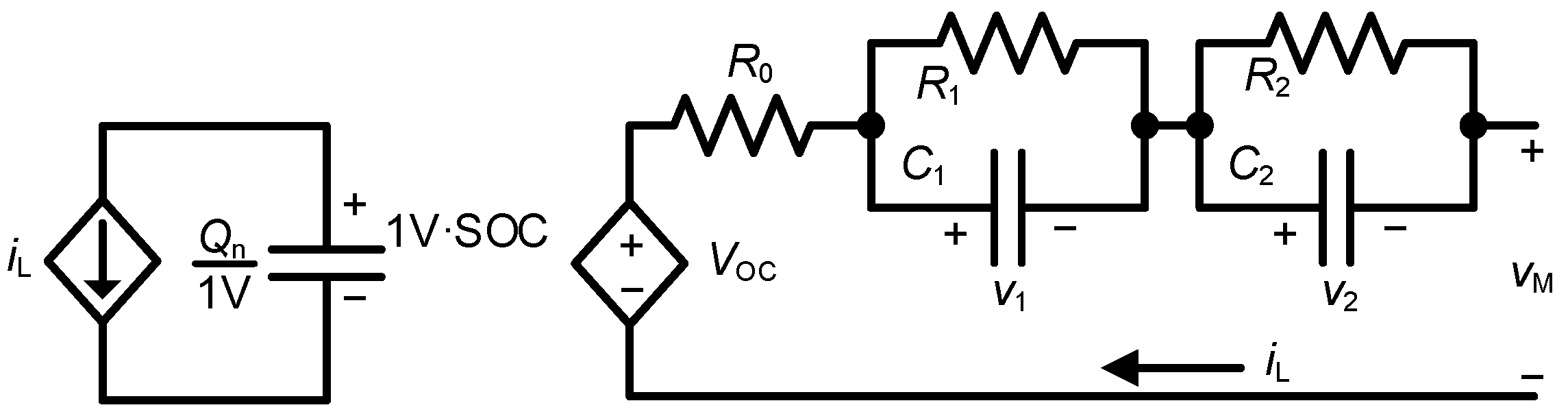
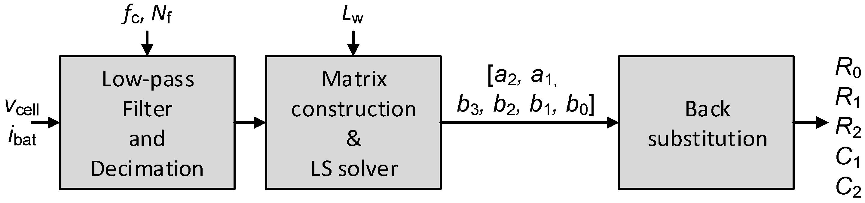
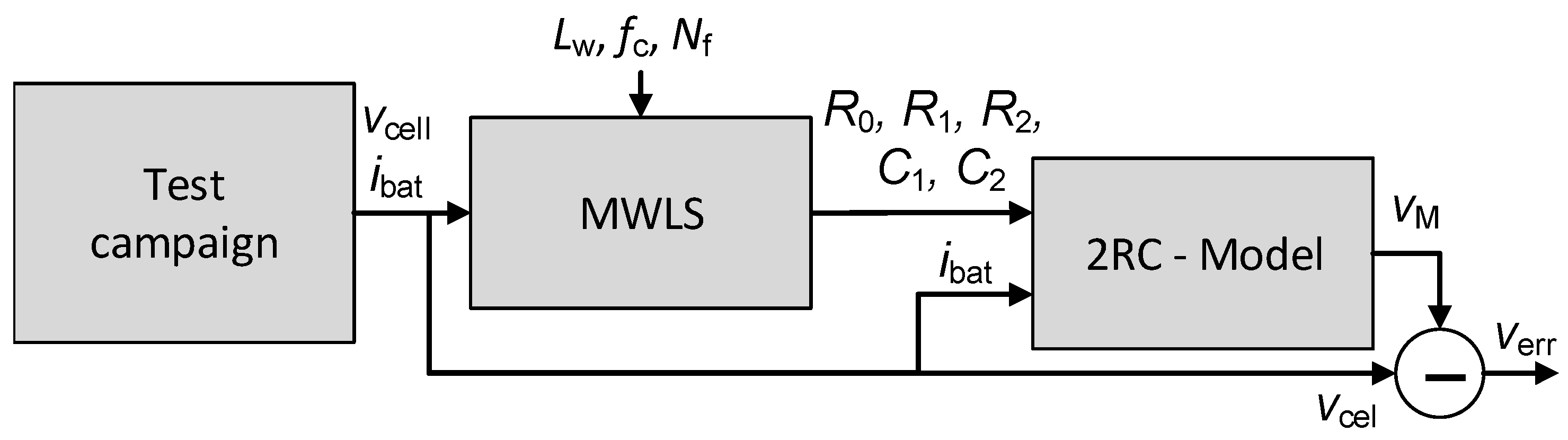
2. Battery Model Parameter Identification

Each cell of the battery pack is modeled using the 2-RC ECM shown in Figure 1.
The model consists of two parts: the left-hand side tracks the cell SOC, while the right-hand one estimates the cell voltage. The cell SOC is obtained as a voltage difference across a capacitor, the value of which is equal to the cell capacity Q n expressed in Coulomb and divided by 1 V . The evaluated SOC is the input signal of the controlled voltage generator V OC that implements the relationship between the open circuit voltage (OCV) and the SOC. V OC is series-connected with a resistance R 0 that models the internal ohmic resistance and two RC groups. The voltage drops generated by R 1 and C 1 and by R 2 and C 2 mimic the fast and the slow cell voltage relaxations, respectively. The state space equations of the model are reported in (1), where τ 1 = R 1 C 1 and τ 2 = R 2 C 2 .
d S O C d t = i L Q n d v 1 d t = v 1 τ 1 + i L C 1 d v 2 d t = v 2 τ 2 + i L C 2 V M = V OC R 0 i L v 1 v 2
In general, the cell model parameters vary with the operating conditions (namely SOC and temperature) and aging of the battery. The aim is to identify the parameters inside a time window, the optimal length of which will be discussed later. Here, we just point out that the OCV–SOC relationship is linearized, while the model parameters are assumed constant inside the identification window. The latter is moved over time to track the parameter variations when the operating conditions and aging of the battery change.
The first step in deriving the identification algorithm is to transform the cell voltage V M in the Laplace domain as:
V M ( s ) = α 0 α 1 I L ( s ) s Q n R 0 I L ( s ) R 1 I L ( s ) 1 + R 1 C 1 s R 2 I L ( s ) 1 + R 2 C 2 s ,
in which the OCV–SOC relationship is linearized by:
V OC = α 0 + α 1 S O C ( s ) ,
where α 0 and α 1 are additional linearization parameters that change with the identification window. Equation (2) can be rewritten in the discrete-time domain using the bilinear transform (4), thus obtaining Equation (5), where T is the sampling time, Y is the cell voltage, and U is the cell current.
s 2 T 1 z 1 1 + z 1
Y ( z 1 ) α 0 U ( z 1 ) = b 3 z 3 + b 2 z 2 + b 1 z 1 + b 0 a 3 z 3 + a 2 z 2 + a 1 z 1 + 1
The detailed equations of b 0 , b 1 , b 2 , b 3 , a 1 , a 2 , and a 3 are reported in Appendix A. It can be seen that the coefficients a 1 , a 2 , and a 3 only depend on τ 1 and τ 2 and that 1 + a 1 + a 2 + a 3 is equal to zero. Therefore, the coefficient a 3 can be substituted with ( 1 + a 1 + a 2 ) in Equation (5), yielding the third-order autoregressive exogenous (ARX) model shown below.
y ( k ) y ( k 3 ) = a 2 ( y ( k 3 ) y ( k 2 ) ) + a 1 ( y ( k 3 ) y ( k 1 ) ) + b 0 u ( k ) + b 1 u ( k 1 ) + b 2 u ( k 2 ) + b 3 u ( k 3 )
The ARX model in Equation (6) is evaluated at M sampling points ( k [ k 0 , k 0 + M 1 ] , which correspond to the identification window starting at the sampling time k 0 . The M equations obtained form a linear system b = A x , where b R M holds the M values of y ( k ) y ( k 3 ) , x is the vector of the variables [ a 1 , a 2 , b 0 , b 1 , b 2 , b 3 ] T , and A R M x 6 is the coefficient matrix filled with the voltage and current values sampled at discrete times from k 0 3 to k 0 + M 1 . As M is chosen to be greater than 6, the system is overdetermined and is solved using the least squares method (LS). The variables a 1 , a 2 , b 0 , b 1 , b 2 , and b 3 thus obtained are used to retrieve the ECM parameters by inverting the equations in Appendix A. The identification window is shifted at each estimation step, i.e., k 0 . This approach is usually known as MWLS, and its block diagram is shown in Figure 2.
The MWLS accuracy depends on the time window length L w = M T [21]. In fact, L w should be long enough to track the voltage dynamics of the RC groups so that R 1 , C 1 , R 2 , and C 2 are observable. A longer L w can be obtained by increasing M. However, larger values of M lead to bigger A matrices and consequently to higher computational costs of the MWLS algorithm. A good trade trade-off between complexity and accuracy has been found for M equal to 30, as shown in [15]. Therefore, a sufficiently long value of L w can be obtained by increasing the sampling time T in the moving window, which is usually longer than the sampling time used in BMSs to acquire the cell voltage v cell and the battery current i bat . Thus, the inputs of the MWLS are obtained by decimating the signals acquired by the BMS. This process imposes a preventive low-pass filtering of the acquired voltage and current signals to limit their bandwidth before decimation, according to the Shannon’s sampling theorem.

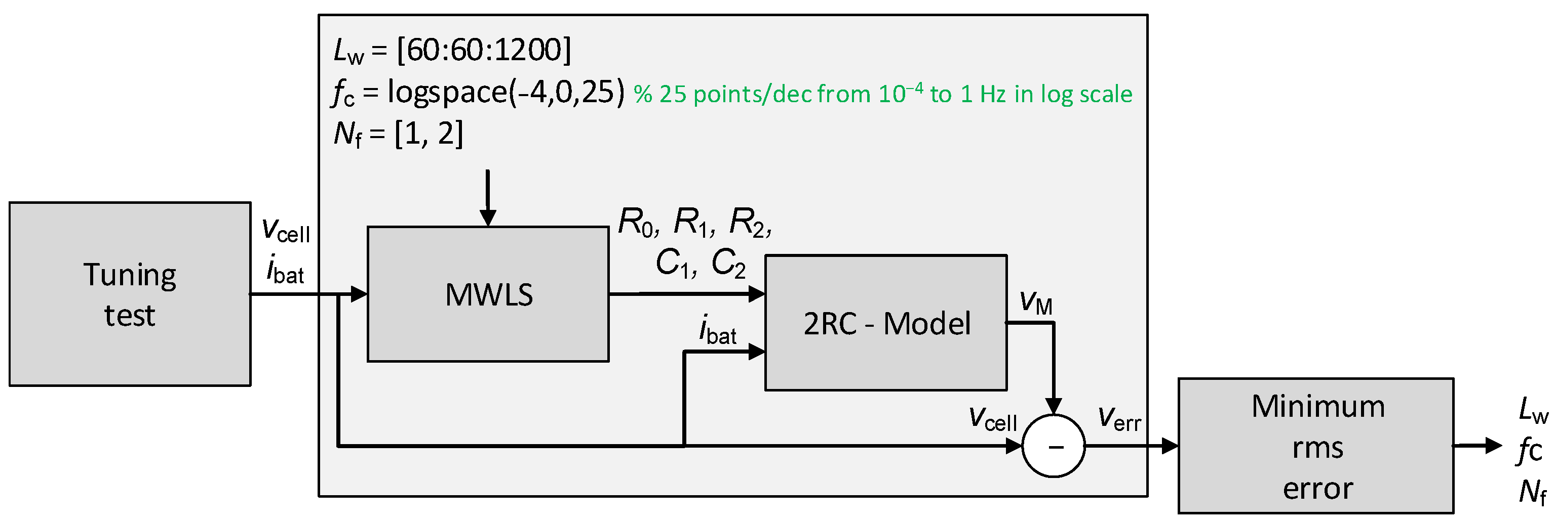
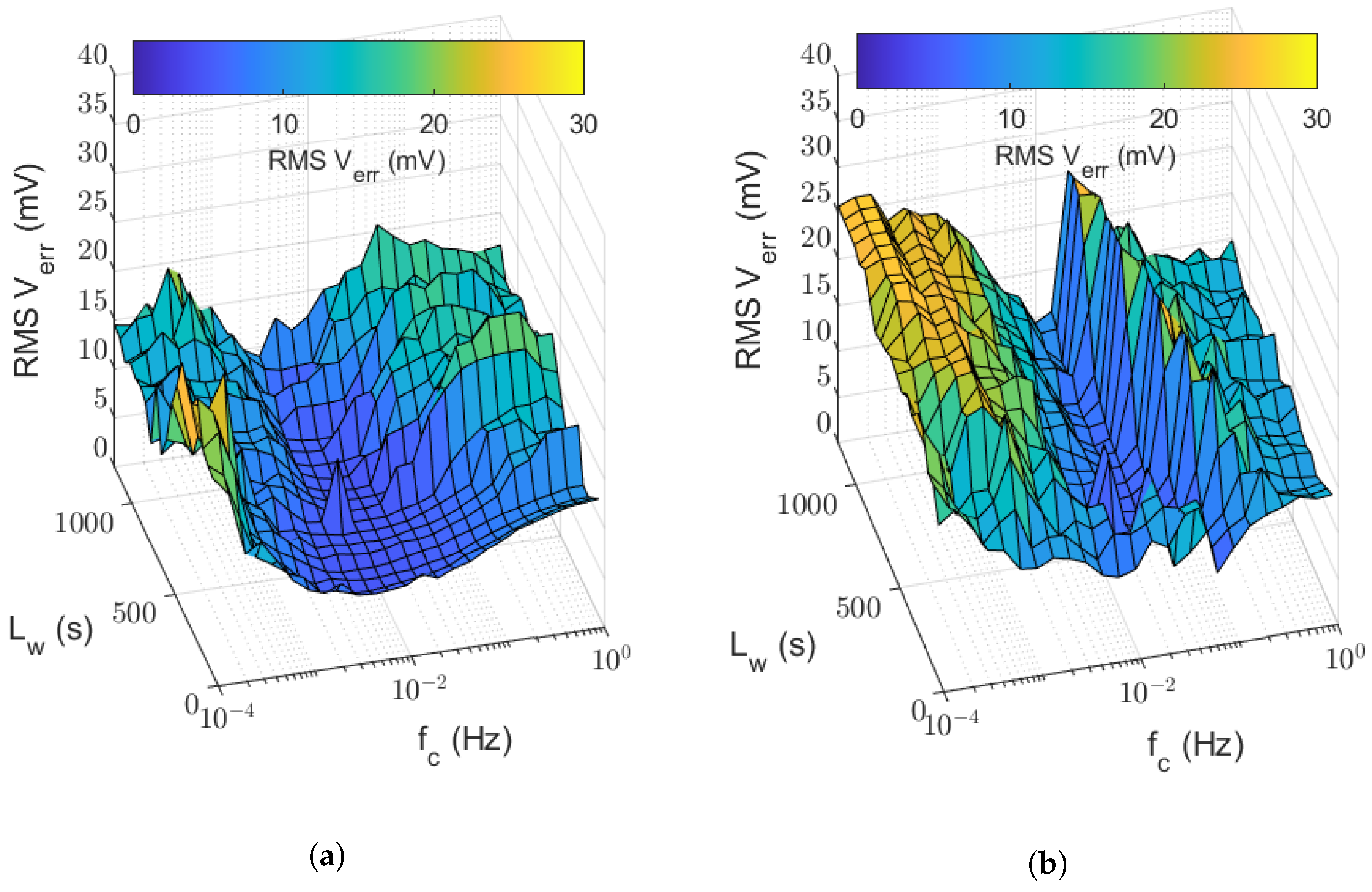
Tuning Procedure of the MWLS Identification Algorithm

The MWLS algorithm requires the appropriate tuning of its parameters to obtain an accurate estimation of the cell model parameters [21]. L w , the low-pass filter cut-off frequency f c , and order N f are the MWLS parameters that are optimized with the tuning procedure proposed in [21], which consists of the following steps:
  • Define a reasonable range for each MWLS parameter;
  • Choose, for each parameter, a reasonable number of possible values in the range previously defined;
  • Run the MWLS algorithm on the measured voltage and current of a battery cell in a test with a load current profile typical of the target application with each possible parameter value combination;
  • Simulate the cell model with the ECM parameters identified in each MWLS execution using the same load current profile;
  • Calculate the RMS error between the measured and simulated cell voltages for each MWLS execution;
  • Select the best combination of L w , f c , and N f as the triplet of values that minimizes the RMS error.

3. Tuning of the MWLS Algorithm for an Electric Vehicle Battery

Real data from an electric vehicle with a battery composed of 108 series-connected cells with 60 Ah capacity are used to tune and validate the MWLS algorithm. The application of the previously described tuning procedure is shown in Figure 3, where the tuning test consists of the current and voltage profiles of cell #1 acquired during a test drive. As shown in Figure 4, the battery is discharged from the initial SOC value of around 90% to 13% in about 4 h , with a rest time of about 30 min when the battery SOC reaches 50%. The average discharge current, excluding the rest period, is around 13 A .
The reasonable ranges of the MWLS parameters have been obtained from both theoretical and empirical considerations. In particular, L w is upper-bounded by the assumption that the ECM parameters are considered constant within the identification window. SOC is the cause of the fastest ECM parameter variations. Limiting the SOC variation in the identification window to below 10% allows this assumption to hold with good approximation [22]. Moreover, the linearization of the OCV–SOC relationship in each identification window is also a good approximation if the SOC variation is limited to 10% [20]. Thus, the maximum value of L w is set to 20 min , which corresponds to a SOC variation of about 7% at the mean discharge current value. Moreover, the f c parameter should be chosen low enough to satisfy the Shannon theorem ( f c 1 / ( 2 T ) ), thus f c M / ( 2 L w ) , but not too low in order not to cancel out the battery voltage dynamics that are captured by the 2-RC groups. However, the ranges chosen for L w , f c , and N f are kept larger than the minimum ones because the tuning procedure is performed offline in the cloud and then its execution time is not a limiting factor. For this reason, the L w range runs from 60 to 1200 s with steps of 60 s , f c goes from 10 4 to 1 Hz following a logarithmic scale with 25 points per decade, and the order of the low-pass N f is set to either 1 or 2.
The MWLS algorithm is executed on the cell current and voltage profiles reported in Figure 4 for each possible combination of the parameter values. The obtained ECM parameters are then used to calculate the predicted cell voltage. The RMS error between the measured and the predicted cell voltage is used to quantify the quality of the identified ECM parameters.
Figure 5a,b show the RMS errors obtained with the explored combinations of L w and f c for N f equal to 1 and 2, respectively. First, we observe that the minimum value of the RMS error is very similar in the two cases, i.e., 4.9   mV (at f c min = 4.6   mHz and L w min = 240   s ) and 5 mV (at f c min = 31.6   mHz and L w min = 180   s ) for the first- and second-order filter, respectively. However, as shown in Figure 5, the surface plot related to the first-order filter shows a larger flat zone around the minimum point compared to what happens to the second-order filter. In fact, considering an octave variation of the f c and L w before and after the minimum point coordinates (i.e., f c [ 0.5 f c min , 2 f c min ] and L w [ 0.5 L w min , 2 L w min ] ), the mean value of the RMS error is 5.4   mV and 9.7   mV for the first- and second-order filter, respectively. This aspect supports the choice of the first-order filter, as it is more robust against variation in the MWLS operating conditions, and its implementation is inherently simpler. Finally, we note that both the RMS error and the MWLS parameters obtained for the first-order filter are in line with the ones reported in [21], where a minimum RMS error of 15 mV is achieved with f c min = 5   mHz and L w min = 210   s .
The MWLS parameters obtained from the first cell are then used to identify the model parameters of the other 107 battery cells by running the algorithm on the individual voltage and current profiles. The RMS error found for each cell model varies in a range from 4.6 to 4.9   mV . Moreover, Figure 6 shows the mean value and the span between the minimum and maximum of the model resistances as a function of the SOC for the 108 battery cells.
Figure 7 shows the distribution of the identified model resistances R 0 and R t = R 0 + R 1 + R 2 for all the battery cells at 50% of SOC. The resistance distributions are fitted with a normal function as suggested by the literature [23], obtaining the mean μ and standard deviation σ values. A relative coefficient of variation, k = σ / μ , is usually calculated to represent the spread of the resistance values around their mean value. The k coefficients of R 0 and R t resistances at 50% of SOC are 1.83% and 1.79%, respectively. These values are in accordance with the literature values for nickel manganese cobalt oxide (NMC) cells [24].

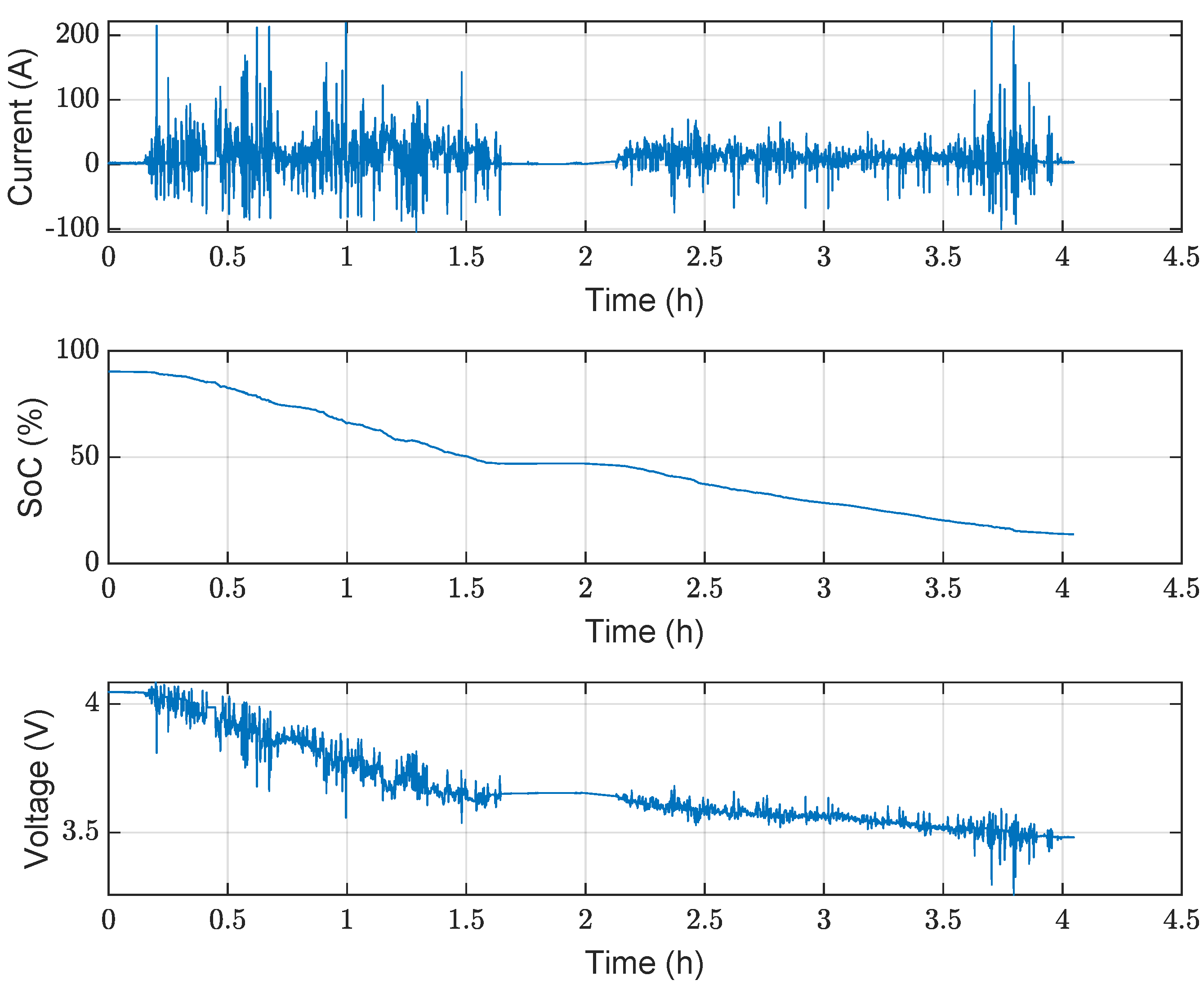
4. Experimental Test Campaign

The MWLS algorithm tuned according to the procedure described in the previous section is applied to 10 road test profiles, the characteristics of which are summarized in Table 1. The investigated profiles were extracted from the experimental daily data collected in the cloud during eight months of electric vehicle driving tests. The test profiles were selected to have large SOC ranges and different current profiles in order to obtain a broader validation of the algorithm.
The model estimation error is calculated by comparing the real acquired voltage to the simulated one with the battery model, whose parameters are identified and tracked by the MWLS algorithm. This test procedure is summarized in Figure 8.
Figure 9a shows the minimum, mean, and maximum values of the RMS and MAE errors of the 108 battery cells for each test. The MAE error is calculated as the average value of the absolute difference between the model and the measured cell voltages. The mean RMS errors obtained by these tests are obviously higher than those found during the tuning procedure. Nevertheless, they are still rather low, being around 0.3% of the nominal cell voltage of 3.6   V , i.e., 11 mV . In addition, the voltage errors seem not to depend on either the driving profile or the season, nor do they increase with time, showing the ability of the MWLS algorithm to accurately track the cell model parameters. The last statement is supported by the evolution of the total cell resistance reported in Figure 9b, as tracked by the MWLS algorithm. Even if the time of operation of the test vehicle is too short to show appreciable aging of the battery, the slightly increasing trend of the total resistance visible in the figure has been caught by the parameter tracking algorithm. In particular, the total resistance goes from about 1.3 to 1.8   m Ω in about 140 cycles (1 cycle for working day in 28 weeks), showing a mean resistance increase of about 0.27% for each cycle. This value is comparable with the literature, in which a cycle SOC ranges from about 90% down to 15%, as shown in [25]. Furthermore, the cell model parameters tracked by the algorithm could be loaded back to the battery, relieving the BMS of the heavy computational load due to parameter identification and allowing a more accurate local estimation of the battery state.

5. Comparison with Literature Data

The results obtained in this work are compared with the literature data in Table 2. The table reports literature studies that address the problem of model parameter identification for different battery models applying different approaches.
For example, an adaptive dual unscented Kalman filter (ADUKF) is used to develop an identification algorithm to estimate the parameters of a 1-RC ECM in [26]. The algorithm is applied to the dynamic stress test (DST) and the Federal Urban Driving Schedule (FUDS), obtaining an RMS error of 10.3   mV and 9.4   mV , respectively. The forgetting factor recursive least squares (FFRLS) technique is instead adopted in [27] to design an estimation parameter algorithm for 1-RC ECM. The authors use the New European Driving Cycle (NEDC) to test the algorithm, obtaining an RMS error of 12.2   mV . Time domain parameter extraction is combined with a decoupled recursive least squares (TD-DRLS) algorithm to estimate the parameters of a 2-RC ECM model in [29]. The DST and FUDS driving cycles are used to assess the TD-DRLS algorithm, achieving RMS errors of 9.1   mV and 9.7   mV , respectively. The SOC and the parameters of a 2-RC ECM with hysteresis are estimated using fixed memory recursive least squares combined with a sigma-point Kalman filter (FMRLS-SPKF) in [30]. The FMRLS-SPKF algorithm is assessed using the DST and FUDS driving cycles, obtaining RMS errors of 8.7   mV and 12.7   mV , respectively. The errors reported in [26,27,28,29,30] are in line with those achieved by our algorithm. However, the load test profiles are applied in controlled environments, and the cell current and voltage are measured with laboratory instruments in the literature. Instead, the current and voltage quantities of our work are directly acquired by the real BMS of the vehicle during road driving tests with lower accuracy and higher noise.

6. Conclusions

This work presents the procedure for the optimization of an algorithm used to identify the parameters of the electrical circuit model of a battery cell with 2-RC relaxation groups. The algorithm applies the MWLS technique and benefits of the cloud computing concept. In fact, the real data coming from a test vehicle are uploaded to the Stellantis-CRF cloud, and the algorithm is executed on them, offline from the BMS, to find the best set of algorithm parameters. The tuning procedure consists of finding the minimum voltage estimation error by exploring all possible combinations of the algorithm parameters, confined to given and reasonable ranges. The parameters that lead to the minimum error are thus selected as golden values for the algorithm. Then, the tuned MWLS algorithm is applied to data from eight months of road tests as uploaded to the cloud by the BMS. The results show that the tuned MWLS algorithm is able to identify the cell model parameters in such a way as to obtain voltage estimation errors that are very small and comparable with literature data obtained in laboratory experiments. Finally, the tracking of the total cell resistance shows a slight increase through time, consistent with the first signs of battery aging.

Author Contributions

Conceptualization, R.D.R., N.N., R.R., R.T. and F.B.; methodology, R.D.R., N.N., N.V, R.T. and F.B.; software, R.D.R. and S.A.; validation, R.D.R. and N.V.; data curation, R.D.R. and S.A.; writing—original draft preparation, R.D.R., N.N., R.R. and R.S.; writing—review and editing, R.D.R., N.N., R.S., R.T. and F.B.; supervision, R.R., R.S., R.T. and F.B.; project administration, F.B. and R.T.; funding acquisition, F.B., R.S. and R.T. All authors have read and agreed to the published version of the manuscript.

Funding

This research was partially funded by the European Union’s Horizon 2020 research and innovation program under grant agreement no. 875131 and by the Italian Ministry of University and Research (MUR) in the framework of the FoReLab project (Departments of Excellence).

Institutional Review Board Statement

Not applicable.

Informed Consent Statement

Not applicable.

Data Availability Statement

The data presented in this study are available on request from the corresponding authors.

Conflicts of Interest

The authors declare no conflict of interest.

Appendix A

The appendix reports the detailed equations that describe the coefficients a 1 , a 2 , a 3 , b 0 , b 1 , b 2 , and b 3 of Equation (5).
a 1 = 2 T τ 1 + 2 T τ 2 + 12 τ 1 τ 2 T 2 T + 2 τ 1 T + 2 τ 2 a 2 = 2 T τ 1 + 2 T τ 2 12 τ 1 τ 2 + T 2 T + 2 τ 1 T + 2 τ 2 a 3 = T 2 τ 1 T 2 τ 2 T + 2 τ 1 T + 2 τ 2
b 0 = α 1 T 3 k 2 T 2 + k 1 T + 8 Q n R 0 τ 1 τ 2 k 3 b 1 = 3 α 1 T 3 + k 2 T 2 + k 1 T + 24 Q n R 0 τ 1 τ 2 k 3 b 2 = 3 α 1 T 3 + k 2 T 2 k 1 T + 24 Q n R 0 τ 1 τ 2 k 3 b 3 = α 1 T 3 + k 2 T 2 + k 1 T 8 Q n R 0 τ 1 τ 2 k 3 k 1 = 4 Q n R 0 τ 1 + 4 Q n R 0 τ 2 + 4 Q n R 1 τ 2 + 4 Q n R 2 τ 1 + 4 α 1 τ 1 τ 2 k 2 = 2 Q n R 0 2 Q n R 1 2 Q n R 2 2 α 1 τ 1 2 α 1 τ 2 k 3 = 2 Q n T + 2 τ 1 T + 2 τ 2

References

  1. Zhao, Y.; Wang, Z.; Shen, Z.J.M.; Zhang, L.; Dorrell, D.G.; Sun, F. Big data-driven decoupling framework enabling quantitative assessments of electric vehicle performance degradation. Appl. Energy 2022, 327, 120083. [Google Scholar] [CrossRef]
  2. Li, S.; He, H.; Wei, Z.; Zhao, P. Edge computing for vehicle battery management: Cloud-based online state estimation. J. Energy Storage 2022, 55, 105502. [Google Scholar] [CrossRef]
  3. Wei, Z.; Yang, X.; Li, Y.; He, H.; Li, W.; Sauer, D.U. Machine learning-based fast charging of lithium-ion battery by perceiving and regulating internal microscopic states. Energy Storage Mater. 2023, 56, 62–75. [Google Scholar] [CrossRef]
  4. Koleti, U.R.; Bui, T.N.M.; Dinh, T.Q.; Marco, J. The Development of Optimal Charging Protocols for Lithium-Ion Batteries to Reduce Lithium Plating. J. Energy Storage 2021, 39, 102573. [Google Scholar] [CrossRef]
  5. Burns, J.C.; Stevens, D.A.; Dahn, J.R. In-Situ Detection of Lithium Plating Using High Precision Coulometry. J. Electrochem. Soc. 2015, 162, A959–A964. [Google Scholar] [CrossRef]
  6. Mohajer, S.; Lanusse, P.; Sabatier, J.; Cois, O. Design of a Model-based Fractional-Order Controller for Optimal Charging of Batteries. IFAC-PapersOnLine 2018, 51, 97–102. [Google Scholar] [CrossRef]
  7. Vo, T.T.; Chen, X.; Shen, W.; Kapoor, A. New charging strategy for lithium-ion batteries based on the integration of Taguchi method and state of charge estimation. J. Power Sources 2015, 273, 413–422. [Google Scholar] [CrossRef]
  8. Perez, H.E.; Hu, X.; Dey, S.; Moura, S.J. Optimal Charging of Li-Ion Batteries with Coupled Electro-Thermal-Aging Dynamics. IEEE Trans. Veh. Technol. 2017, 66, 7761–7770. [Google Scholar] [CrossRef]
  9. Abdollahi, A.; Han, X.; Avvari, G.V.; Raghunathan, N.; Balasingam, B.; Pattipati, K.R.; Bar-Shalom, Y. Optimal battery charging, Part I: Minimizing time-to-charge, energy loss, and temperature rise for OCV-resistance battery model. J. Power Sources 2016, 303, 388–398. [Google Scholar] [CrossRef]
  10. Hwang, G.; Sitapure, N.; Moon, J.; Lee, H.; Hwang, S.; Sang-Il Kwon, J. Model predictive control of Lithium-ion batteries: Development of optimal charging profile for reduced intracycle capacity fade using an enhanced single particle model (SPM) with first-principled chemical/mechanical degradation mechanisms. Chem. Eng. J. 2022, 435, 134768. [Google Scholar] [CrossRef]
  11. Barzacchi, L.; Lagnoni, M.; Rienzo, R.D.; Bertei, A.; Baronti, F. Enabling early detection of lithium-ion battery degradation by linking electrochemical properties to equivalent circuit model parameters. J. Energy Storage 2022, 50, 104213. [Google Scholar] [CrossRef]
  12. Wang, Z.; Feng, G.; Zhen, D.; Gu, F.; Ball, A. A review on online state of charge and state of health estimation for lithium-ion batteries in electric vehicles. Energy Rep. 2021, 7, 5141–5161. [Google Scholar] [CrossRef]
  13. Noura, N.; Boulon, L.; Jemeï, S. A Review of Battery State of Health Estimation Methods: Hybrid Electric Vehicle Challenges. World Electr. Veh. J. 2020, 11, 66. [Google Scholar] [CrossRef]
  14. Restaino, R.; Zamboni, W. Comparing particle filter and extended kalman filter for battery State-Of-Charge estimation. In Proceedings of the IECON 2012—38th Annual Conference on IEEE Industrial Electronics Society, Montreal, QC, Canada, 25–28 October 2012; pp. 4018–4023. [Google Scholar] [CrossRef]
  15. Morello, R.; Di Rienzo, R.; Roncella, R.; Saletti, R.; Baronti, F. Hardware-in-the-Loop Platform for Assessing Battery State Estimators in Electric Vehicles. IEEE Access 2018, 6, 68210–68220. [Google Scholar] [CrossRef]
  16. Zhu, W.; Zhou, X.; Cao, M.; Wang, Y.; Zhang, T. The Cloud-End Collaboration Battery Management System with Accurate State-of-Charge Estimation for Large-Scale Lithium-ion Battery System. In Proceedings of the 2022 8th International Conference on Big Data and Information Analytics (BigDIA), Guiyang, China, 24–25 August 2022; pp. 199–204. [Google Scholar] [CrossRef]
  17. Shi, D.; Zhao, J.; Wang, Z.; Zhao, H.; Eze, C.; Wang, J.; Lian, Y.; Burke, A.F. Cloud-Based Deep Learning for Co-Estimation of Battery State of Charge and State of Health. Energies 2023, 16, 3855. [Google Scholar] [CrossRef]
  18. Mondal, A.; Routray, A.; Puravankara, S. Parameter identification and co-estimation of state-of-charge of Li-ion battery in real-time on Internet-of-Things platform. J. Energy Storage 2022, 51, 104370. [Google Scholar] [CrossRef]
  19. Li, W.; Rentemeister, M.; Badeda, J.; Jöst, D.; Schulte, D.; Sauer, D.U. Digital twin for battery systems: Cloud battery management system with online state-of-charge and state-of-health estimation. J. Energy Storage 2020, 30, 101557. [Google Scholar] [CrossRef]
  20. Rahimi-Eichi, H.; Baronti, F.; Chow, M.Y. Online Adaptive Parameter Identification and State-of-Charge Coestimation for Lithium-Polymer Battery Cells. IEEE Trans. Ind. Electron. 2014, 61, 2053–2061. [Google Scholar] [CrossRef]
  21. Morello, R.; Di Rienzo, R.; Roncella, R.; Saletti, R.; Baronti, F. Tuning of Moving Window Least Squares-based algorithm for online battery parameter estimation. In Proceedings of the 2017 14th International Conference on Synthesis, Modeling, Analysis and Simulation Methods and Applications to Circuit Design (SMACD), Giardini Naxos, Italy, 12–15 June 2017; pp. 1–4. [Google Scholar] [CrossRef]
  22. Bruch, M.; Millet, L.; Kowal, J.; Vetter, M. Novel method for the parameterization of a reliable equivalent circuit model for the precise simulation of a battery cell’s electric behavior. J. Power Sources 2021, 490, 229513. [Google Scholar] [CrossRef]
  23. Paul, S.; Diegelmann, C.; Kabza, H.; Tillmetz, W. Analysis of ageing inhomogeneities in lithium-ion battery systems. J. Power Sources 2013, 239, 642–650. [Google Scholar] [CrossRef]
  24. Schindler, M.; Sturm, J.; Ludwig, S.; Schmitt, J.; Jossen, A. Evolution of initial cell-to-cell variations during a three-year production cycle. eTransportation 2021, 8, 100102. [Google Scholar] [CrossRef]
  25. Ecker, M.; Nieto, N.; Käbitz, S.; Schmalstieg, J.; Blanke, H.; Warnecke, A.; Sauer, D.U. Calendar and cycle life study of Li(NiMnCo)O2-based 18650 lithium-ion batteries. J. Power Sources 2014, 248, 839–851. [Google Scholar] [CrossRef]
  26. Peng, N.; Zhang, S.; Guo, X.; Zhang, X. Online parameters identification and state of charge estimation for lithium-ion batteries using improved adaptive dual unscented Kalman filter. Int. J. Energy Res. 2021, 45, 975–990. [Google Scholar] [CrossRef]
  27. Lao, Z.; Xia, B.; Wang, W.; Sun, W.; Lai, Y.; Wang, M. A Novel Method for Lithium-Ion Battery Online Parameter Identification Based on Variable Forgetting Factor Recursive Least Squares. Energies 2018, 11, 1358. [Google Scholar] [CrossRef]
  28. Li, L.; Zhu, H.; Zhou, A.; Hu, M.; Fu, C.; Qin, D. A Novel Online Parameter Identification Algorithm for Fractional-Order Equivalent Circuit Model of Lithium-Ion Batteries. Int. J. Electrochem. Sci. 2020, 15, 6863–6879. [Google Scholar] [CrossRef]
  29. Pai, H.Y.; Liu, Y.H.; Ye, S.P. Online estimation of lithium-ion battery equivalent circuit model parameters and state of charge using time-domain assisted decoupled recursive least squares technique. J. Energy Storage 2023, 62, 106901. [Google Scholar] [CrossRef]
  30. Sun, C.; Lin, H.; Cai, H.; Gao, M.; Zhu, C.; He, Z. Improved parameter identification and state-of-charge estimation for lithium-ion battery with fixed memory recursive least squares and sigma-point Kalman filter. Electrochim. Acta 2021, 387, 138501. [Google Scholar] [CrossRef]
Figure 1. Electric equivalent model with 2-RC groups.
Batteries 09 00486 g001
Figure 2. Block diagram of moving window least squares approach.
Batteries 09 00486 g002
Figure 3. Block diagram of the tuning procedure of the MWLS algorithm.
Batteries 09 00486 g003
Figure 4. Current, state-of-charge, and voltage profiles of battery cell #1 used to tune the MWLS algorithm.
Batteries 09 00486 g004
Figure 5. RMS error of the voltage predicted by the ECM, as a function of the identification window length L w , the cut-off frequency f c of the filter, and its order. (a) Low-pass filter order N f = 1 . (b) Low-pass filter order N f = 2 .
Batteries 09 00486 g005
Figure 6. Values of ECM resistances identified by applying the tuned MWLS to all the battery cells. Mean value is depicted as a solid line, while minimum and maximum values are reported as vertical bars.
Batteries 09 00486 g006
Figure 7. Distribution of the resistances R 0 (a) and R t = R 0 + R 1 + R 2 (b) of all battery cells estimated by the MWLS algorithm at 50% of SOC and their fitting with a normal distribution function.
Batteries 09 00486 g007
Figure 8. Block diagram of the MWLS algorithm test procedure.
Batteries 09 00486 g008
Figure 9. Maximum, mean, and minimum RMS and MAE errors (a) and R t = R 0 + R 1 + R 2 (b) of the 108 battery cells for each test reported in Table 1.
Batteries 09 00486 g009
Table 1. Tests selected from about eight months of driving tests to characterize the MWLS algorithm.
SOC (%)
Test #DayLength (h)Mean Current (A)StartEndMean Speed (km h−1)Distance (km)
128 April 20201.528.493.119.866.698.7
225 May 20202.221.892.88.464.9140.8
38 June 20202.317.989.719.253.6121.9
420 June 20203.812.392.613.143163.6
529 June 20202.320.194.810.1NA 1NA 1
64 July 20204.311.89310.236.1154
717 August 20204.111.794.712.5NA 1NA 1
84 September 20203.412.89316.535.8120.7
927 September 20202.11989.214.549.1105.1
1016 November 20202.119.395.714.747.298.7
1 Data not available (GPS error).
Table 2. Comparison of the obtained results with the literature.
WorkBattery ModelEstimation MethodRMS Error
This workECM with 2-RCMWLS11 mV (Road data)
[26]ECM with 1-RCADUKF 10.3   mV (DST)
9.4   mV (FUDS)
[27]ECM with 1-RCFFRLS 12.2   mV (NEDC)
[28]Fractional Order ECMRLS 8.02   mV (DST)
6.37   mV (FUDS)
[29]ECM with 2-RCTD-DRLS 9.7   mV (FUDS)
9.1   mV (DST)
[30]ECM with 2-RCFMRLS-SPKF 12.7   mV (FUDS)
and Hysteresis 8.7   mV (DST)
Disclaimer/Publisher’s Note: The statements, opinions and data contained in all publications are solely those of the individual author(s) and contributor(s) and not of MDPI and/or the editor(s). MDPI and/or the editor(s) disclaim responsibility for any injury to people or property resulting from any ideas, methods, instructions or products referred to in the content.

