
Determination of Internal Temperature Differences for Various Cylindrical Lithium-Ion Batteries Using a Pulse Resistance Approach


Abstract
:1. Introduction
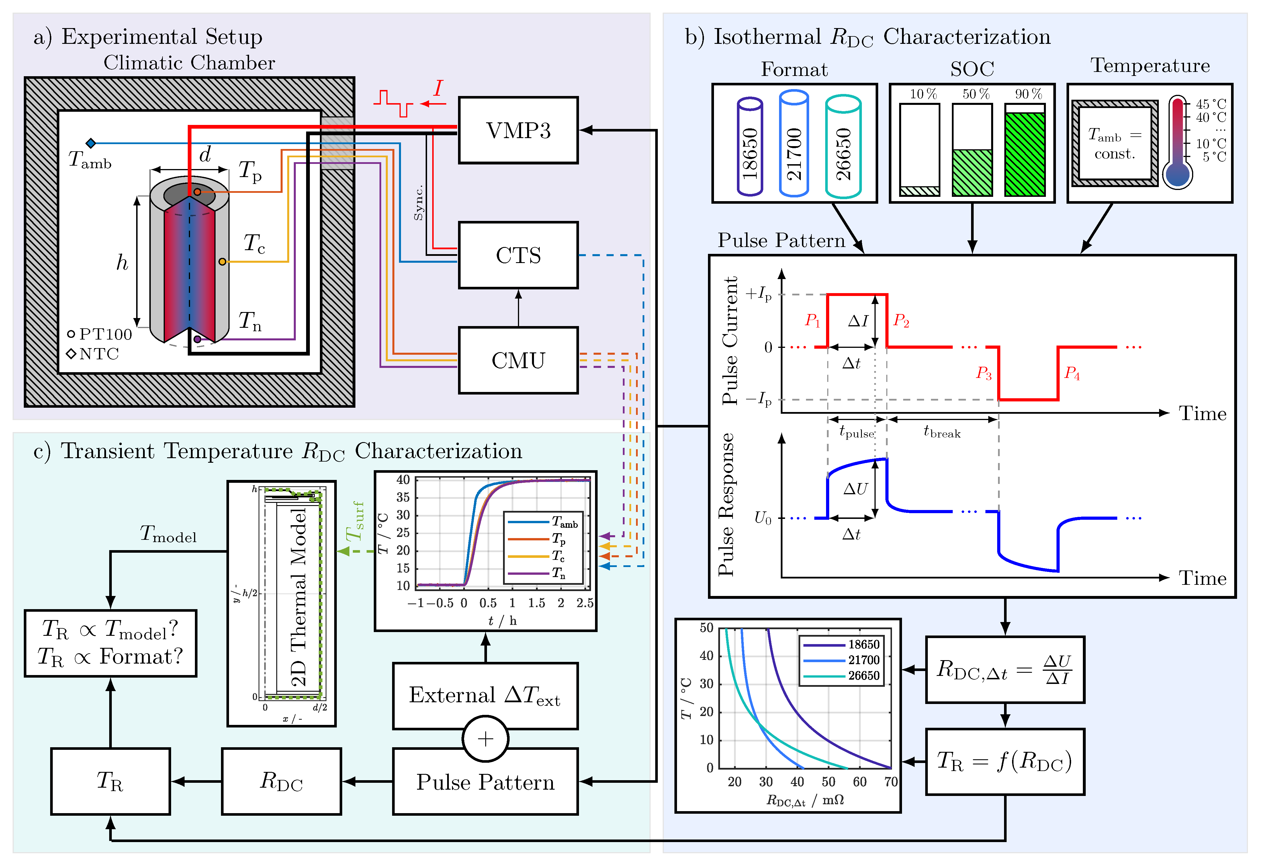
2. Experiment
2.1. Investigated Cells
2.2. Experimental Setup
2.3. Test Procedures
2.3.1. Isothermal Characterization
- (P.1)
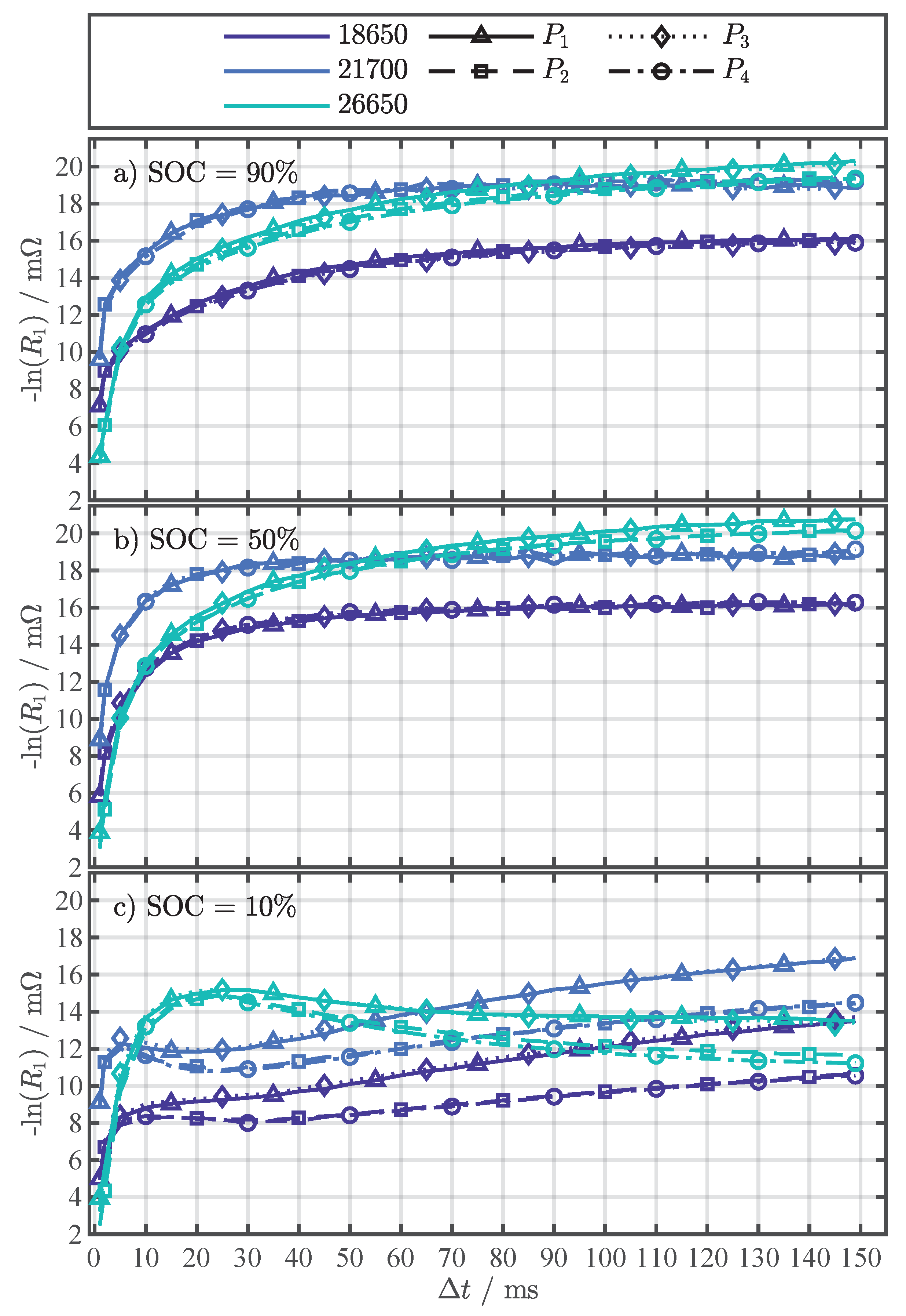
- Our previous analysis in [27] revealed that the optimal evaluation time for the for temperature estimation is in the region of 10 to approximately 100 . To cover this range with margin, the pulse duration () was set to 150 . However, the exact evaluation time () is determined in Section 4.1 with the results listed in Table 4.
- (P.2)
- The continuous pulses may affect each other since LIBs are time-variant systems. The pause between the charging and discharging pulses () was set to 5 , which proved to be long enough to avoid the preceding pulse to affect the following one (see Section 4.1).
- (P.3)
- To analyze the transient temperature behavior (see Section 2.3.2), the cell temperature is changed by externally heating the cell and simultaneously applying current pulses. Internal temperature changes due to heating of the cells through ohmic losses [37] caused by the continuous application of the pulses had to be avoided. Therefore, the pulse current and duration had to be small. The pulse duration with 150 selected in (P.1) is already relatively short. Nevertheless, the current had to be large enough to induce a voltage response with a sufficient signal-to-noise ratio (SNR) to avoid inaccurate measurements. The trade-off resulted in a pulse current of . Taking the resistance values for from Table 2 into account, the resulting heat generation of the applied pulses is less than for each cell.
2.3.2. Transient Temperature Characterization
3. 2D Thermal Model
4. Results & Discussion
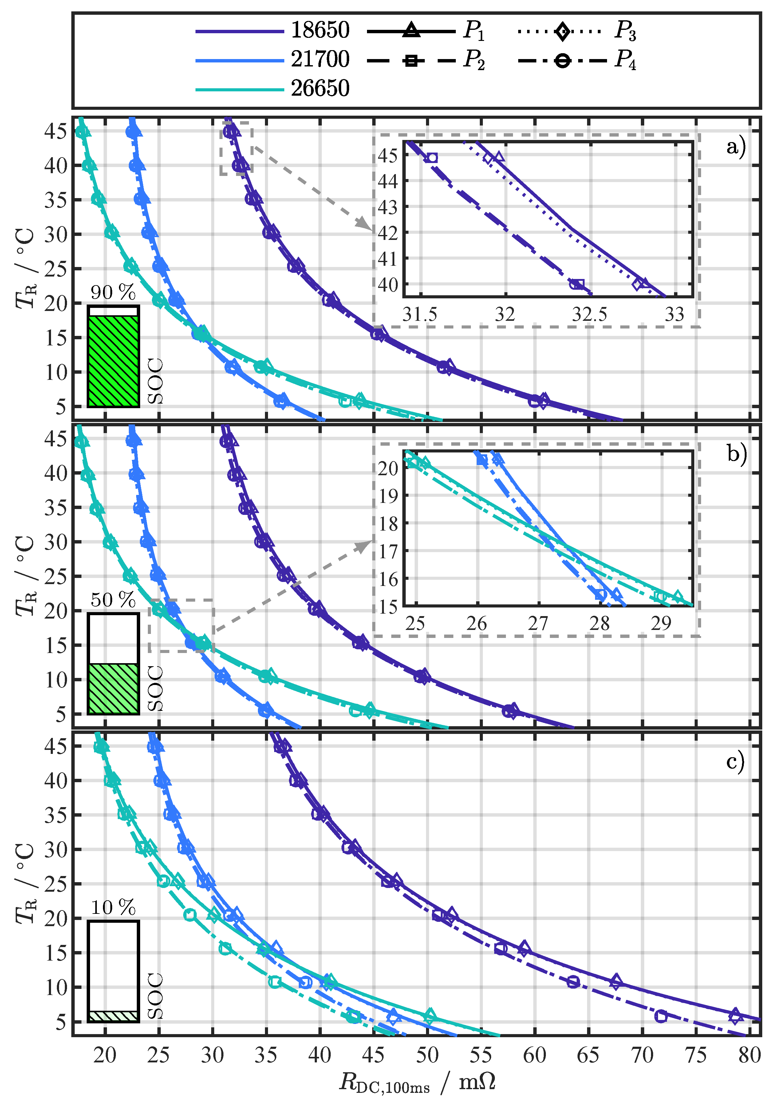
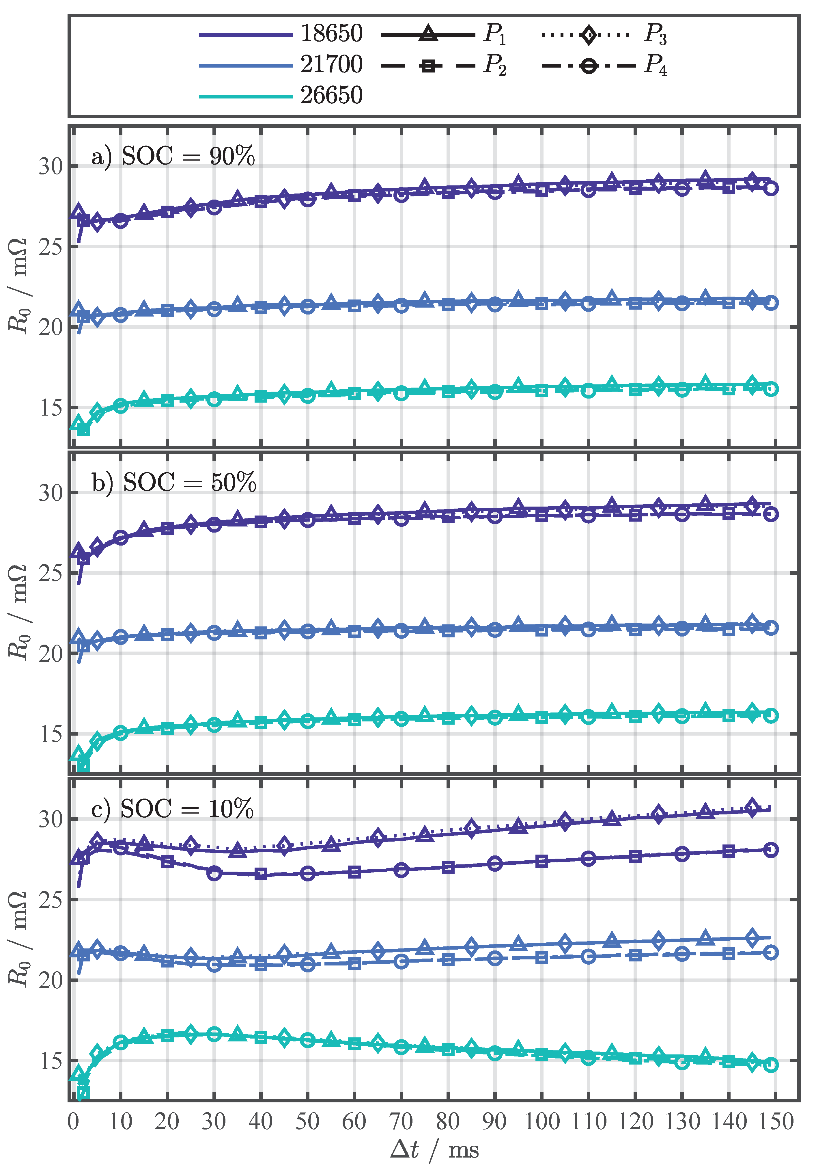
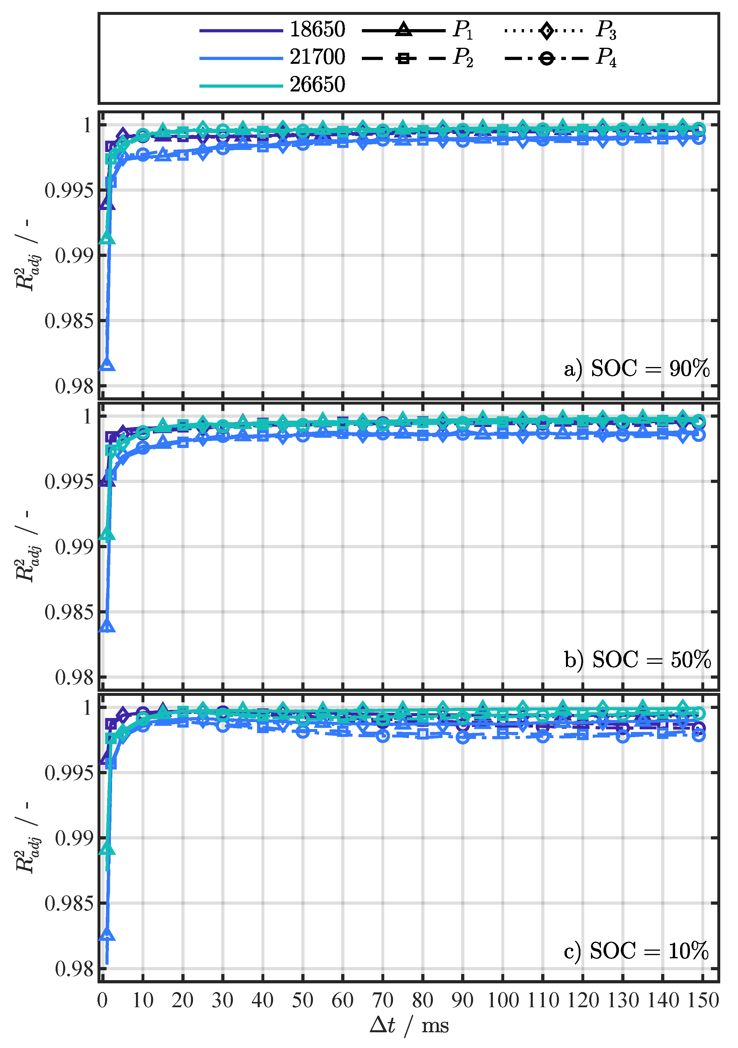
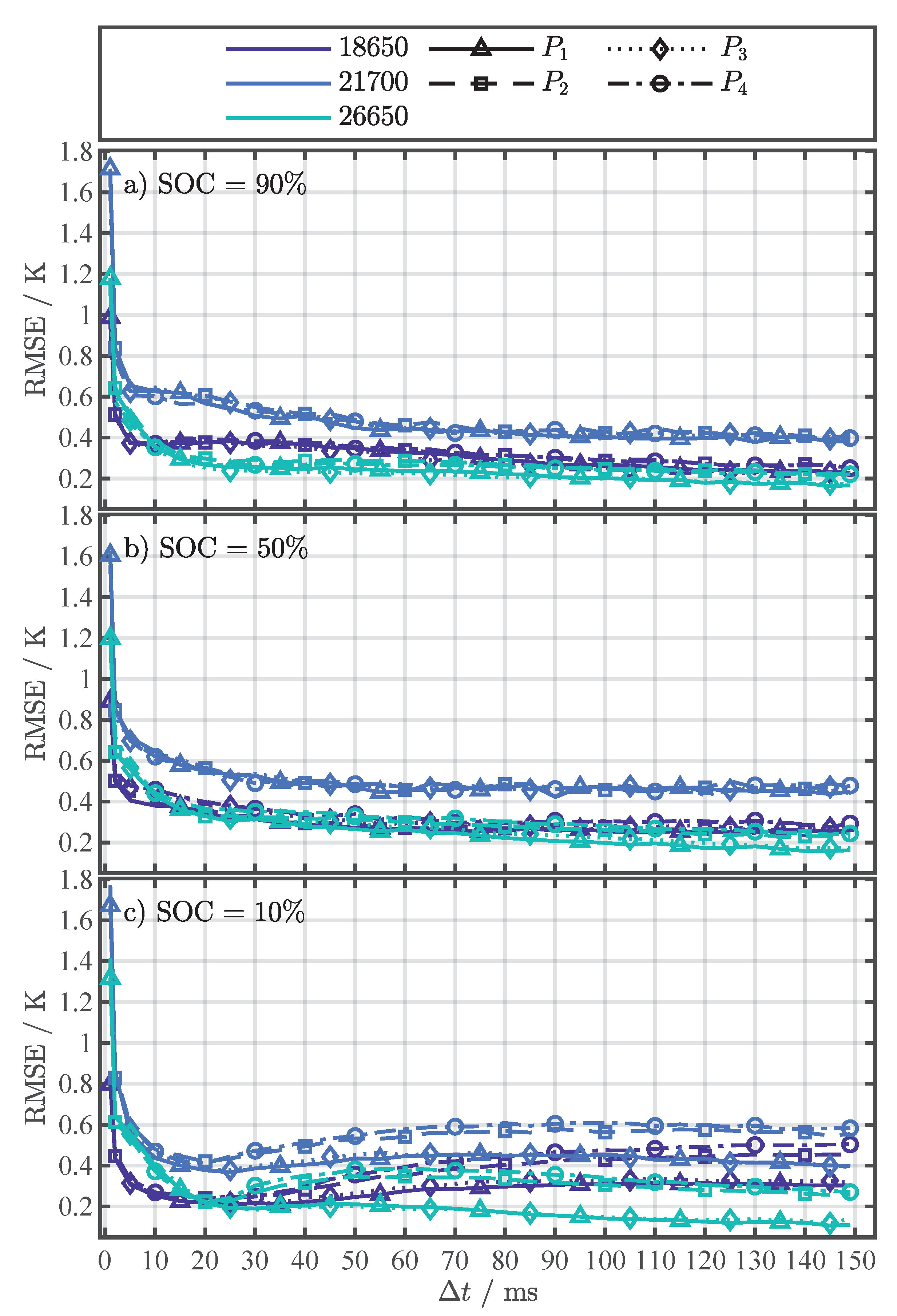
4.1. Isothermal Characterization
- (E.1)
- Ohmic losses, due to limiting electronic/ionic conductivity of the current collectors, the electrolyte, the active materials of the electrodes, and additives, such as carbon black.
- (E.2)
- Contact losses, attributed to contact resistance between one of the electrodes and the current collector, as well as from particle-to-particle contacts.
- (E.3)
- Interface losses, related to the charge transfer at the electrodes, as well as the contribution of the solid electrolyte interface (SEI).
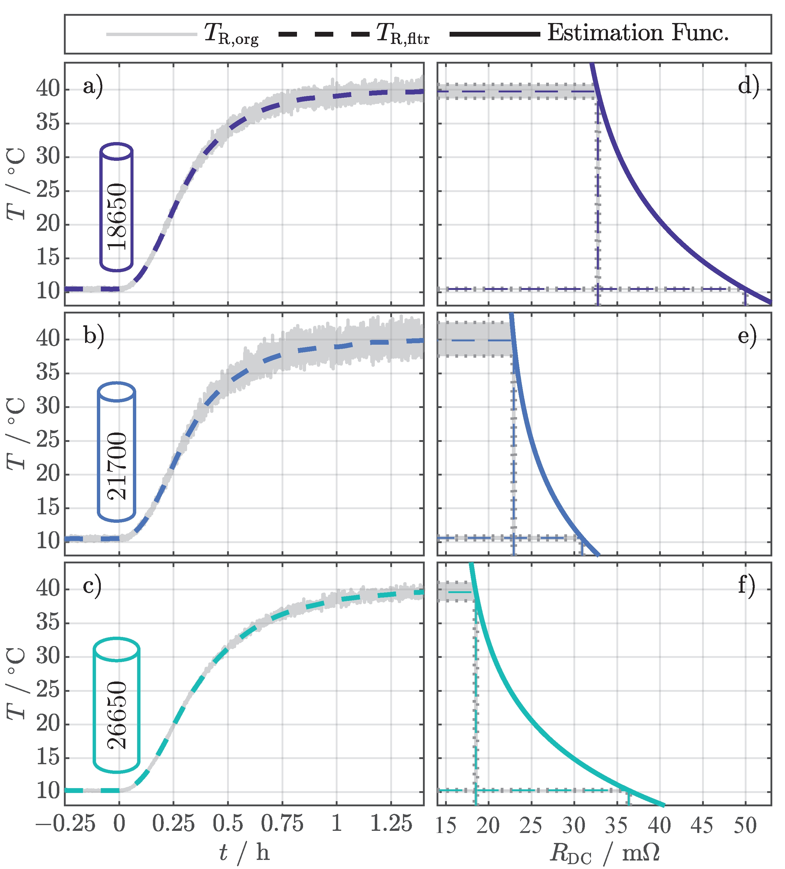
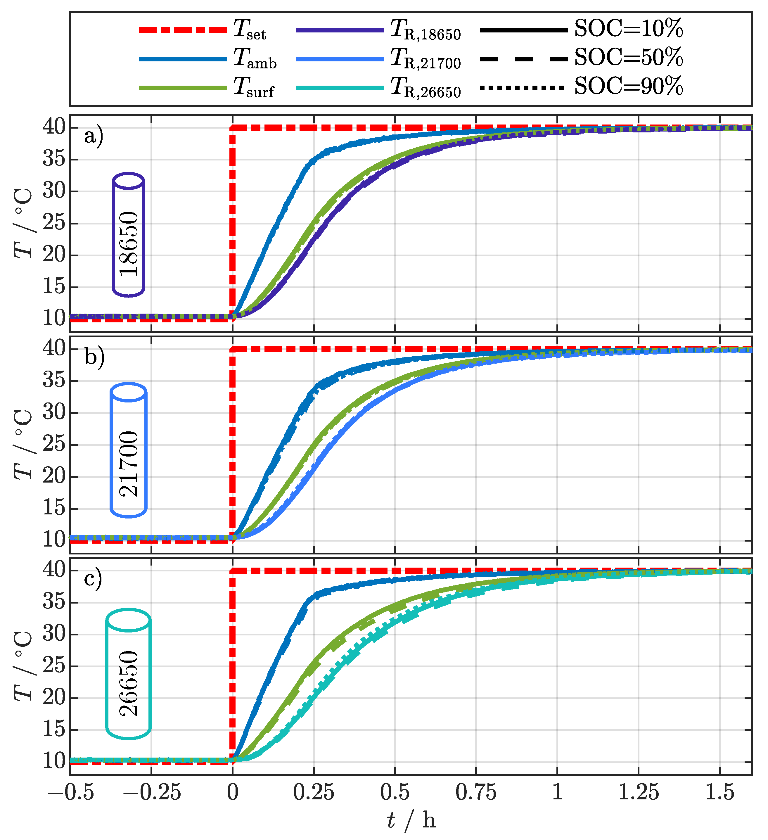
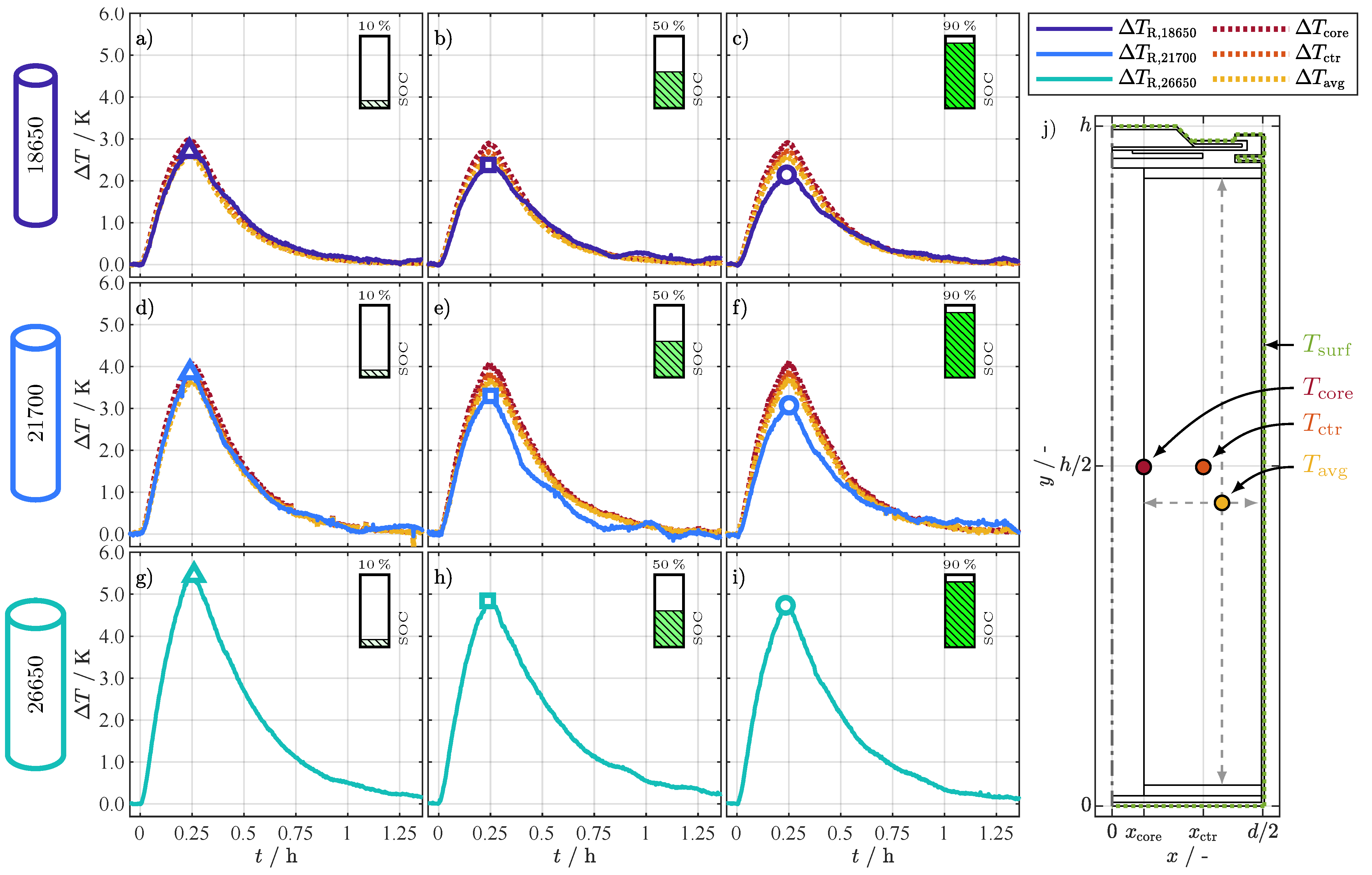
4.2. Transient Temperature Characterization
4.3. Internal Temperature: Model versus
- (R.1)
- Although the simulation parameters are for the same pristine cell type, they were not determined for exactly the same cell and thus might slightly differ between the cells used in [31] to parameterize the 2D thermal model and the ones used in this study. Also, the SOC points in the study by Steinhardt et al. [31] do not exactly match the SOC points investigated in this study. Since the thermal conductivity of a LIB is dependent on the SOC [47], the parameter deviation in thermal conductivity might partly cause the deviation between the simulation and .
- (R.2)
- The 2D thermal model does not consider thermal conductivity changes related to mechanical changes. The jelly roll expands when the cell is charged [48] and the contact area and pressure between the layers in the jelly roll and between the jelly roll and the metal casing of the cell increases. Several studies [49,50] showed that increased compression reduces the thermal contact resistance, leading to improved thermal conductivity and therefore reducing the difference between surface and core temperature.
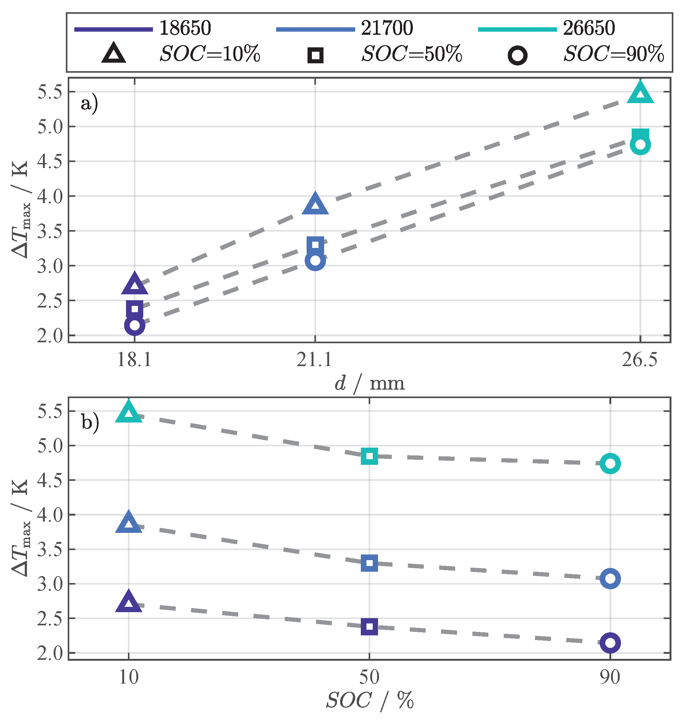
4.4. Internal Temperature: Cell Geometry & State of Charge
5. Summary & Conclusions
- The can be utilized to determine the internal cell temperature for different cell chemistries and cylindrical cell formats.
- The comparison with the 2D thermal model shows that most likely represents the average jelly roll temperature (). Thus, offers an advantage over conventional temperature sensors, which only determine the surface temperature at one point of the cell.
- An important point regarding the applicability is the temperature range, for which -based methods are applicable. As shown in Figure 3, the accuracy of the method strongly depends on the slope of the estimation function (Equation (4)), which steadily increases with rising temperatures. For this reason, correspondingly precise measurement hardware for the current and voltage monitoring of the BMS is a prerequisite to avoid large temperature estimation errors in the elevated temperature range.
Author Contributions
Funding
Data Availability Statement
Conflicts of Interest
Abbreviations
| BMS | battery management system |
| CC | constant current |
| CMU | cell measurement unit |
| CTS | cell test system |
| CV | constant voltage |
| DVA | differential voltage analysis |
| EIS | electrochemical impedance spectroscopy |
| FEM | finite element model |
| LIB | lithium-ion battery |
| LMO | LiMnO |
| NMC | nickel manganese cobalt oxide |
| NTC | negative temperature coefficient |
| OCV | open-circuit voltage |
| R-Square | |
| adjusted R-Square | |
| direct current resistance | |
| RMSE | root mean square error |
| SEI | solid electrolyte interface |
| SNR | signal-to-noise ratio |
| SOC | state of charge |
| SOH | state of health |
| SSE | sum of square error |
| SST | total sum of squares |
| ambient temperature | |
| simulated average jelly roll temperature | |
| temperature at the center of the cell | |
| temperature simulated at half of the cell height and at the core of the jelly roll | |
| temperature simulated at half of the cell height and at the center of the jelly roll | |
| external change in temperature | |
| temperature at the negative terminal | |
| temperature at the positive terminal | |
| temperature indicated by the | |
| temperature difference between and the for the 18650 cell | |
| temperature difference between and the for the 21700 cell | |
| temperature difference between and the for the 26650 cell | |
| averaged surface temperature |
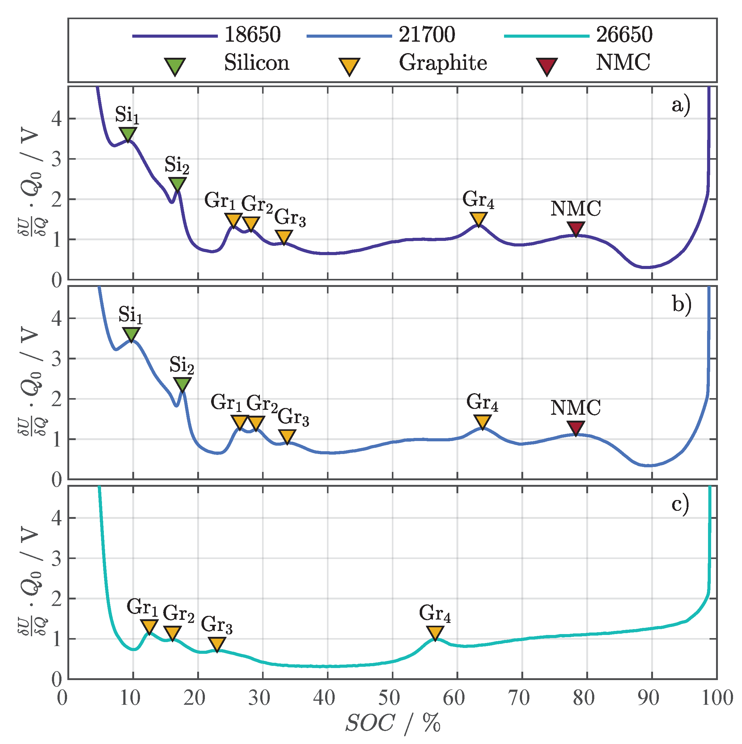
Appendix A. Differential Voltage Analysis

Appendix B. Function Parameters


Appendix C. Fitting Quality & Error
- -
- the sum of square error (SSE) in Equation (A1) describes the total deviation of the response values of the fit from the measured response values ,
- -
- the total sum of squares (SST) in Equation (A2) describes the total deviation of the mean from the measured response values ,
- -
- the general in Equation (A3) determines how successful the fit is in explaining the variation of the data,
- -
- and the adjusted R-Square statistic in Equation (A4) considers the number of fitted model variables m in addition to the number of response values n.


References
- Ma, S.; Jiang, M.; Tao, P.; Song, C.; Wu, J.; Wang, J.; Deng, T.; Shang, W. Temperature effect and thermal impact in lithium-ion batteries: A review. Prog. Nat. Sci. Mater. Int. 2018, 28, 653–666. [Google Scholar] [CrossRef]
- Morello, R.; Di Rienzo, R.; Roncella, R.; Saletti, R.; Schwarz, R.; Lorentz, V.; Hoedemaekers, E.; Rosca, B.; Baronti, F. Advances in Li-Ion Battery Management for Electric Vehicles. In Proceedings of the IECON 2018-44th Annual Conference of the IEEE Industrial Electronics Society, Washington, DC, USA, 21–23 October 2018; IEEE: Piscataway, NJ, USA, 2018; pp. 4949–4955. [Google Scholar] [CrossRef] [Green Version]
- Alipour, M.; Ziebert, C.; Conte, F.V.; Kizilel, R. A Review on Temperature-Dependent Electrochemical Properties, Aging, and Performance of Lithium-Ion Cells. Batteries 2020, 6, 35. [Google Scholar] [CrossRef]
- Raijmakers, L.; Danilov, D.L.; Eichel, R.A.; Notten, P. A review on various temperature-indication methods for Li-ion batteries. Appl. Energy 2019, 240, 918–945. [Google Scholar] [CrossRef]
- Beelen, H.; Mundaragi Shivakumar, K.; Raijmakers, L.; Donkers, M.; Bergveld, H.J. Towards impedance–based temperature estimation for Li–ion battery packs. Int. J. Energy Res. 2020, 44, 2889–2908. [Google Scholar] [CrossRef]
- Richardson, R.R.; Zhao, S.; Howey, D.A. On-board monitoring of 2-D spatially-resolved temperatures in cylindrical lithium-ion batteries: Part II. State estimation via impedance-based temperature sensing. J. Power Sources 2016, 327, 726–735. [Google Scholar] [CrossRef] [Green Version]
- Liu, X.; Ai, W.; Naylor Marlow, M.; Patel, Y.; Wu, B. The effect of cell-to-cell variations and thermal gradients on the performance and degradation of lithium-ion battery packs. Appl. Energy 2019, 248, 489–499. [Google Scholar] [CrossRef]
- Srinivasan, R. Monitoring dynamic thermal behavior of the carbon anode in a lithium-ion cell using a four-probe technique. J. Power Sources 2012, 198, 351–358. [Google Scholar] [CrossRef]
- Carkhuff, B.G.; Demirev, P.A.; Srinivasan, R. Impedance-Based Battery Management System for Safety Monitoring of Lithium-Ion Batteries. IEEE Trans. Ind. Electron. 2018, 65, 6497–6504. [Google Scholar] [CrossRef]
- Srinivasan, R.; Carkhuff, B.G.; Butler, M.H.; Baisden, A.C. Instantaneous measurement of the internal temperature in lithium-ion rechargeable cells. Electrochim. Acta 2011, 56, 6198–6204. [Google Scholar] [CrossRef]
- Schmidt, J.P.; Arnold, S.; Loges, A.; Werner, D.; Wetzel, T.; Ivers-Tiffée, E. Measurement of the internal cell temperature via impedance: Evaluation and application of a new method. J. Power Sources 2013, 243, 110–117. [Google Scholar] [CrossRef]
- Raijmakers, L.; Danilov, D.L.; van Lammeren, J.; Lammers, M.; Notten, P. Sensorless battery temperature measurements based on electrochemical impedance spectroscopy. J. Power Sources 2014, 247, 539–544. [Google Scholar] [CrossRef]
- Beelen, H.; Raijmakers, L.; Donkers, M.; Notten, P.; Bergveld, H.J. An Improved Impedance-Based Temperature Estimation Method for Li-ion. IFAC-PapersOnLine 2015, 48, 383–388. [Google Scholar] [CrossRef]
- Spinner, N.S.; Love, C.T.; Rose-Pehrsson, S.L.; Tuttle, S.G. Expanding the Operational Limits of the Single-Point Impedance Diagnostic for Internal Temperature Monitoring of Lithium-ion Batteries. Electrochim. Acta 2015, 174, 488–493. [Google Scholar] [CrossRef]
- Sun, J.; Wei, G.; Pei, L.; Lu, R.; Song, K.; Wu, C.; Zhu, C. Online Internal Temperature Estimation for Lithium-Ion Batteries Based on Kalman Filter. Energies 2015, 8, 4400–4415. [Google Scholar] [CrossRef] [Green Version]
- Zhu, J.G.; Sun, Z.C.; Wei, X.Z.; Dai, H.F. A new lithium-ion battery internal temperature on-line estimate method based on electrochemical impedance spectroscopy measurement. J. Power Sources 2015, 274, 990–1004. [Google Scholar] [CrossRef]
- Zhu, J.; Sun, Z.; Wei, X.; Dai, H. Battery Internal Temperature Estimation for LiFePO4 Battery Based on Impedance Phase Shift under Operating Conditions. Energies 2017, 10, 60. [Google Scholar] [CrossRef] [Green Version]
- Srinivasan, R.; Demirev, P.A.; Carkhuff, B.G. Rapid monitoring of impedance phase shifts in lithium-ion batteries for hazard prevention. J. Power Sources 2018, 405, 30–36. [Google Scholar] [CrossRef]
- Wang, L.; Lu, D.; Song, M.; Zhao, X.; Li, G. Instantaneous estimation of internal temperature in lithium–ion battery by impedance measurement. Int. J. Energy Res. 2020, 44, 3082–3097. [Google Scholar] [CrossRef]
- Raijmakers, L.H.J.; Danilov, D.L.; van Lammeren, J.P.M.; Lammers, T.J.G.; Bergveld, H.J.; Notten, P.H.L. Non-Zero Intercept Frequency: An Accurate Method to Determine the Integral Temperature of Li-Ion Batteries. IEEE Trans. Ind. Electron. 2016, 63, 3168–3178. [Google Scholar] [CrossRef] [Green Version]
- Haussmann, P.; Melbert, J. Internal Cell Temperature Measurement and Thermal Modeling of Lithium Ion Cells for Automotive Applications by Means of Electrochemical Impedance Spectroscopy. SAE Int. J. Altern. Powertrains 2017, 6, 261–270. [Google Scholar] [CrossRef]
- Wang, X.; Wei, X.; Chen, Q.; Zhu, J.; Dai, H. Lithium-ion battery temperature on-line estimation based on fast impedance calculation. J. Energy Storage 2019, 26, 100952. [Google Scholar] [CrossRef]
- Richardson, R.R.; Ireland, P.T.; Howey, D.A. Battery internal temperature estimation by combined impedance and surface temperature measurement. J. Power Sources 2014, 265, 254–261. [Google Scholar] [CrossRef]
- Richardson, R.R.; Howey, D.A. Sensorless Battery Internal Temperature Estimation Using a Kalman Filter With Impedance Measurement. IEEE Trans. Sustain. Energy 2015, 6, 1190–1199. [Google Scholar] [CrossRef] [Green Version]
- Xie, Y.; Li, W.; Hu, X.; Lin, X.; Zhang, Y.; Dan, D.; Feng, F.; Liu, B.; Li, K. An Enhanced Online Temperature Estimation for Lithium-Ion Batteries. IEEE Trans. Transp. Electrif. 2020, 6, 375–390. [Google Scholar] [CrossRef]
- Forgez, C.; Vinh Do, D.; Friedrich, G.; Morcrette, M.; Delacourt, C. Thermal modeling of a cylindrical LiFePO4/graphite lithium-ion battery. J. Power Sources 2010, 195, 2961–2968. [Google Scholar] [CrossRef]
- Ludwig, S.; Zilberman, I.; Horsche, M.F.; Wohlers, T.; Jossen, A. Pulse resistance based online temperature estimation for lithium-ion cells. J. Power Sources 2021, 490, 229523. [Google Scholar] [CrossRef]
- Ludwig, S.; Zilberman, I.; Oberbauer, A.; Rogge, M.; Fischer, M.; Rehm, M.; Jossen, A. Adaptive method for sensorless temperature estimation over the lifetime of lithium-ion batteries. J. Power Sources 2022, 521, 230864. [Google Scholar] [CrossRef]
- Tranter, T.G.; Timms, R.; Shearing, P.R.; Brett, D.J.L. Communication—Prediction of Thermal Issues for Larger Format 4680 Cylindrical Cells and Their Mitigation with Enhanced Current Collection. J. Electrochem. Soc. 2020, 167, 160544. [Google Scholar] [CrossRef]
- Tomaszewska, A.; Chu, Z.; Feng, X.; O’Kane, S.; Liu, X.; Chen, J.; Ji, C.; Endler, E.; Li, R.; Liu, L.; et al. Lithium-ion battery fast charging: A review. eTransportation 2019, 1, 100011. [Google Scholar] [CrossRef]
- Steinhardt, M.; Gillich, E.I.; Rheinfeld, A.; Kraft, L.; Spielbauer, M.; Bohlen, O.; Jossen, A. Low-effort determination of heat capacity and thermal conductivity for cylindrical 18650 and 21700 lithium-ion cells. J. Energy Storage 2021, 42, 103065. [Google Scholar] [CrossRef]
- Shenzhen Fest Technology Co., Ltd. Efest IMR 26650 5000mAh 40A Flat Top Battery. Available online: https://www.efestpower.com/index.php?ac=article&at=read&did=448. (accessed on 18 January 2022).
- Popp, H.; Zhang, N.; Jahn, M.; Arrinda, M.; Ritz, S.; Faber, M.; Sauer, D.U.; Azais, P.; Cendoya, I. Ante-mortem analysis, electrical, thermal, and ageing testing of state-of-the-art cylindrical lithium-ion cells. e & i Elektrotechnik und Informationstechnik 2020, 137, 169–176. [Google Scholar] [CrossRef]
- Wei, Y.; Agelin-Chaab, M. Experimental investigation of a novel hybrid cooling method for lithium-ion batteries. Appl. Therm. Eng. 2018, 136, 375–387. [Google Scholar] [CrossRef]
- Wei, Y.; Agelin-Chaab, M. Development and experimental analysis of a hybrid cooling concept for electric vehicle battery packs. J. Energy Storage 2019, 25, 100906. [Google Scholar] [CrossRef]
- Gantenbein, S.; Weiss, M.; Ivers-Tiffée, E. Impedance based time-domain modeling of lithium-ion batteries: Part I. J. Power Sources 2018, 379, 317–327. [Google Scholar] [CrossRef]
- Bernardi, D. A General Energy Balance for Battery Systems. J. Electrochem. Soc. 1985, 132, 5. [Google Scholar] [CrossRef] [Green Version]
- Illig, J.; Ender, M.; Chrobak, T.; Schmidt, J.P.; Klotz, D.; Ivers-Tiffée, E. Separation of Charge Transfer and Contact Resistance in LiFePO 4 -Cathodes by Impedance Modeling. J. Electrochem. Soc. 2012, 159, A952–A960. [Google Scholar] [CrossRef]
- Zhou, X.; Huang, J.; Pan, Z.; Ouyang, M. Impedance characterization of lithium-ion batteries aging under high-temperature cycling: Importance of electrolyte-phase diffusion. J. Power Sources 2019, 426, 216–222. [Google Scholar] [CrossRef]
- Barai, A.; Uddin, K.; Widanage, W.D.; McGordon, A.; Jennings, P. A study of the influence of measurement timescale on internal resistance characterisation methodologies for lithium-ion cells. Sci. Rep. 2018, 8, 21. [Google Scholar] [CrossRef]
- Song, J.Y.; Wang, Y.Y.; Wan, C.C. Conductivity Study of Porous Plasticized Polymer Electrolytes Based on Poly(vinylidene fluoride) A Comparison with Polypropylene Separators. J. Electrochem. Soc. 2000, 147, 3219. [Google Scholar] [CrossRef]
- Suresh, P.; Shukla, A.K.; Munichandraiah, N. Temperature dependence studies of a.c. impedance of lithium-ion cells. J. Appl. Electrochem. 2002, 32, 267–273. [Google Scholar] [CrossRef]
- Muto, S.; Tatsumi, K.; Kojima, Y.; Oka, H.; Kondo, H.; Horibuchi, K.; Ukyo, Y. Effect of Mg-doping on the degradation of LiNiO2-based cathode materials by combined spectroscopic methods. J. Power Sources 2012, 205, 449–455. [Google Scholar] [CrossRef]
- Schranzhofer, H.; Bugajski, J.; Santner, H.J.; Korepp, C.; Möller, K.C.; Besenhard, J.O.; Winter, M.; Sitte, W. Electrochemical impedance spectroscopy study of the SEI formation on graphite and metal electrodes. J. Power Sources 2006, 153, 391–395. [Google Scholar] [CrossRef]
- Raju, N.S.; Bilgic, R.; Edwards, J.E.; Fleer, P.F. Methodology Review: Estimation of Population Validity and Cross-Validity, and the Use of Equal Weights in Prediction. Appl. Psychol. Meas. 1997, 21, 291–305. [Google Scholar] [CrossRef]
- Fuller, T.F. Relaxation Phenomena in Lithium-Ion-Insertion Cells. J. Electrochem. Soc. 1994, 141, 982. [Google Scholar] [CrossRef] [Green Version]
- Maleki, H.; Hallaj, S.A.; Selman, J.R.; Dinwiddie, R.B.; Wang, H. Thermal Properties of Lithium–Ion Battery and Components. J. Electrochem. Soc. 1999, 146, 947–954. [Google Scholar] [CrossRef]
- Willenberg, L.; Dechent, P.; Fuchs, G.; Teuber, M.; Eckert, M.; Graff, M.; Kürten, N.; Sauer, D.U.; Figgemeier, E. The Development of Jelly Roll Deformation in 18650 Lithium-Ion Batteries at Low State of Charge. J. Electrochem. Soc. 2020, 167, 120502. [Google Scholar] [CrossRef]
- Maleki, H.; Selman, J.; Dinwiddie, R.; Wang, H. High thermal conductivity negative electrode material for lithium-ion batteries. J. Power Sources 2001, 94, 26–35. [Google Scholar] [CrossRef]
- Richter, F.; Kjelstrup, S.; Vie, P.J.; Burheim, O.S. Thermal conductivity and internal temperature profiles of Li-ion secondary batteries. J. Power Sources 2017, 359, 592–600. [Google Scholar] [CrossRef] [Green Version]


| # | Reference | Temperature | Cell | System | ||||
|---|---|---|---|---|---|---|---|---|
| Internal Core | Internal Distribution | Average Integral | Capacity | Format | Chemistry Cathode|Anode | |||
| 1 | [8] | A | 53 Ah | prismatic | LCO|Gr | cell | ||
| 2 | [9] | C | Ah | 18650 | ? | 1s2p | ||
| A | ||||||||
| 3 | [2] | x | 34 Ah | prismatic | NMC|? | cell | ||
| 4 | [5] | x | Ah | prismatic | NMC|? | 2s1p | ||
| 5 | [10] | x | 53 Ah | prismatic | LCO|Gr | cell | ||
| Ah | 26650 | LFG|Gr | cell | |||||
| Ah | 18650 | ? | 1s2p | |||||
| 6 | [11] | x | 2 Ah | pouch | LCO+NCA|Gr | cell | ||
| 7 | [12] | x | Ah | 26650 | LFP|Gr | cell | ||
| Ah | cylindrical | NCA|Gr | cell | |||||
| 8 | [13] | x | 90 Ah | ? | LFP|? | cell | ||
| 9 | [14] | x | Ah | 18650 | LCO|? | cell | ||
| 10 | [15] | x | 40 Ah | pouch | LFP|Gr | cell | ||
| 11 | [16] | x | 8 Ah | prismatic | ? | cell | ||
| 12 | [17] | x | 30 Ah | pouch | LFP|Gr | cell | ||
| 13 | [18] | x | 50 Ah | prismatic | LCO|Gr | cell | ||
| Ah | 18650 | ? | 1s2p | |||||
| 3 Ah | 18650 | NMC|? | cell | |||||
| 14 | [19] | x | Ah | 18650 | LFP|? | cell | ||
| 15 | [20] | x | 90 Ah | prismatic | LFP|? | 3s1p | ||
| 16 | [22] | x | 8 Ah | prismatic | LFP|? | cell | ||
| 40 Ah | pouch | LFP|? | cell | |||||
| 17 | [23] | (x) | x | Ah | 26650 | LFP|Gr | cell | |
| 18 | [24] | (x) | x | Ah | 26650 | LFP|Gr | cell | |
| 19 | [6] | x | x | 20 Ah | prismatic | LMO/NMC|? | cell | |
| 20 | [25] | x | Ah | 18650 | ? | cell | ||
| 18650 | 21700 | 26650 | ||
|---|---|---|---|---|
| Identifier | INR18650-MJ1 | INR21700-M50T | IMR26650-V1 | |
| Manufacturer | LG Chem | LG Chem | Efest | |
| Dimensions | 18.1|65.1 [31] | 21.1|70.2 [31] | 26.5|65.2 [32] | |
| ()/ | ||||
| Chemistry | NMC|Gr/Si (a) | NMC|Gr/Si (b) | LMO|Gr (c) | |
| (Cathode|Anode) | ||||
| Capacity () | ||||
| Batch | ||||
| Capacity | ||||
| 0.483% | 0.124% | 0.233% | ||
| Impedance | ||||
| 0.379% | 0.868% | 0.618% | ||
| Parameter | Value |
|---|---|
| Pulse Current () | |
| Pulse Duration () | 150 |
| Break Duration () | 5 |
| SOC | Format | RMSE / K | / ms | |
|---|---|---|---|---|
| 90% | 18650 | 0.223 | 3 | 149 |
| 21700 | 0.378 | 1 | 130 | |
| 26650 | 0.162 | 1 | 145 | |
| 50% | 18650 | 0.248 | 1 | 149 |
| 21700 | 0.423 | 1 | 90 | |
| 26650 | 0.158 | 1 | 145 | |
| 10% | 18650 | 0.208 | 1 | 25 |
| 21700 | 0.367 | 1 | 25 | |
| 26650 | 0.106 | 1 | 145 |
Publisher’s Note: MDPI stays neutral with regard to jurisdictional claims in published maps and institutional affiliations. |
© 2022 by the authors. Licensee MDPI, Basel, Switzerland. This article is an open access article distributed under the terms and conditions of the Creative Commons Attribution (CC BY) license (https://creativecommons.org/licenses/by/4.0/).
Share and Cite
Ludwig, S.; Steinhardt, M.; Jossen, A. Determination of Internal Temperature Differences for Various Cylindrical Lithium-Ion Batteries Using a Pulse Resistance Approach. Batteries 2022, 8, 60. https://doi.org/10.3390/batteries8070060
Ludwig S, Steinhardt M, Jossen A. Determination of Internal Temperature Differences for Various Cylindrical Lithium-Ion Batteries Using a Pulse Resistance Approach. Batteries. 2022; 8(7):60. https://doi.org/10.3390/batteries8070060
Chicago/Turabian StyleLudwig, Sebastian, Marco Steinhardt, and Andreas Jossen. 2022. "Determination of Internal Temperature Differences for Various Cylindrical Lithium-Ion Batteries Using a Pulse Resistance Approach" Batteries 8, no. 7: 60. https://doi.org/10.3390/batteries8070060