Development of a Matlab/Simulink Model for Monitoring Cell State-of-Health and State-of-Charge via Impedance of Lithium-Ion Battery Cells

Abstract

Lithium-ion battery cells not only show different behaviors depending on degradation and charging states, but also overcharge and overdischarge of cells shorten battery life and cause safety problems, thus studies aiming to provide an accurate state of a cell are required. Measurements of battery cell impedance are used for cell SoH and SoC estimation techniques, but it generally takes a long time for a cell in each state to be prepared and cell voltage response is measured when charging and discharging under each condition. This study introduces an electrical equivalent circuit model of lithium-ion cells developed in the MATLAB/Simulink environment. Cell SoC, SoH, temperature, and C-rate are considered for more accurate cell impedance prediction, and the simulation results are verified with the measurement results. The developed model is suitable for use in cell SoC and SoH monitoring studies by successfully outputting cell impedance through real-time prediction of cell voltage during discharge.

1. Introduction

Li-ion battery cells have been widely adopted for reasons such as less self-discharge, less memory effect, higher energy density per weight and volume, stable performance, and longer cycle life compared to other types of secondary batteries. They are used in a variety of systems such as portable electronics [1], electric vehicles [2], spacecraft and aircraft power systems [3], renewable energy systems [4], marine current energy systems [5], stationary energy storage [6], etc. The performance of the battery cell depends on the degree of degradation. In addition, overcharging and overdischarging of battery cells not only cause permanent damage to the cells, but can also cause safety problems [7].

The purpose of this paper is to build a Li-ion battery cell model for the simulation and optimization of cell state-of-health (SoH) [8] and cell state-of-charge (SoC) [9] monitoring methods. This model estimates the continuous impedance of the cell during discharge for state monitoring. In particular, the cell impedance when a multi-sine signal is applied to the cell operating current is simulated. To output cell impedance, the simulation model considers cell SoC, SoH, cell temperature, and operating current.

It takes much time to measure battery cells under different conditions. It generally takes several hours to measure cell behavior during only one charge and discharge cycle and rest between them. In addition, it can take months for cells to be measured in different SoHs. Nevertheless, in most cases a number of cells must be prepared under different conditions (SoC, SoH, temperature, etc.). Cell simulation models greatly reduce the cost of experiments. In addition to the cost of purchasing experimental devices and cells, the use of models can save time for each cell state to be set. This is because simulation results are displayed simply by entering the parameters of each cell state. The results of the cell state estimation algorithm can be compared in a short time with simulations under different conditions before being measured as an experiment. In this paper, a simulation model is created that outputs the cell voltage and cell impedance when two test frequencies are superimposed on the cell operating current.

An appropriate modeling method should be selected, as computational time increases due to increased computational effort along with model complexity. The battery models presented in the literature are mainly classified into three main categories: physics-based electrochemical models, electrical equivalent circuit models, and data-driven models. All three categories are described shortly in the following considering their suitability for the intended purpose.

• Physics-based electrochemical models [10,11,12]

Electrochemical models of batteries are structurally based on the electrochemical processes and reactions inside the cell. These models describe the physical and chemical processes inside the battery cell in greater detail than other models. Therefore, these battery cell models are the most accurate, but they are highly complex and require sufficient knowledge of the cell’s electrochemical processes. For these models to be used in practical applications, very detailed knowledge of the battery cell to be modeled is required as battery-related parameters (e.g., electrode thickness, electrolyte initial salt concentration, total heat capacity, etc.) must be known. Moreover, as these models contain a large number of nonlinear differential equations, the simulation process is time-consuming.

As an alternative to the physics-based modeling method, nonlinear system identification procedures of black-box and gray-box models are used. Electrical equivalent circuit models called gray-box models and data-driven models called black-box models can be classified as empirical models. Empirical models use experimental data to predict battery response. Transfer functions and equations by curve fitting can be used, as well as fuzzy logic and artificial neural networks (ANN).

• Data-driven models

Data-based models belong to the black-box model. It is not necessary to understand the reaction mechanism and characteristics inside the battery cell. Therefore, data-driven approaches are advantageous for estimation of systems for which mathematical models are unknown, have high uncertainty, cannot be modeled by empirical equations, or are not suitable for analysis [13]. Fuzzy logic controllers [14], support vector machines (SVM) [15], genetic algorithms (GA) [16], and neural network (NN) algorithms [17] are used in black-box models. Estimation accuracy is highly dependent on the training data set and training method.

• Electrical equivalent circuit models (ECMs)

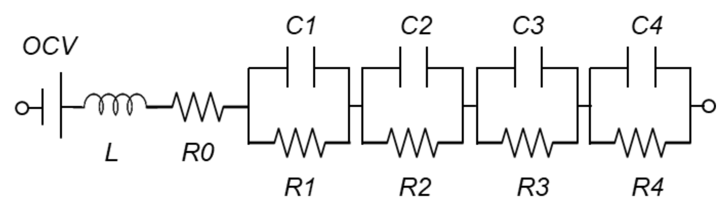
ECMs are also called gray-box models. One important advantage of the gray-box approach is the reduced complexity compared to physics-based electrochemical models. Although the internal electrochemical state of a battery cell is not clearly known, gray-box modeling provides a fast and accurate simulation, suitable for estimating system dynamics and frequency response. The ECMs use linear passive elements that consider the electrical characteristics of the battery cell. These include internal ohmic resistance, polarization resistance, polarization capacitance, inductance, constant phase element, etc. [18]. There are various models of ECM depending on the trade-off between required accuracy and computation time. The parallel connection of resistance and capacitance, called the RC element, is one of the most common elements in electrochemical impedance modeling. Randles et al. established an impedance model structure called the so-called Randles circuit [19,20,21]. Depending on the shape of the measured cell impedance spectrum, it also includes series ohmic resistance, Warburg diffusion elements, and several RC elements [22,23,24]. In addition, if the standard RC network is not suitable for simulating battery characteristics over the entire frequency range, constant phase elements (CPE) are used instead of capacitors in the RC network [25,26,27]. However, oversimplified dynamic models may not include features such as nonlinear equilibrium potential, rate-dependent capacity, and the effects of temperature.

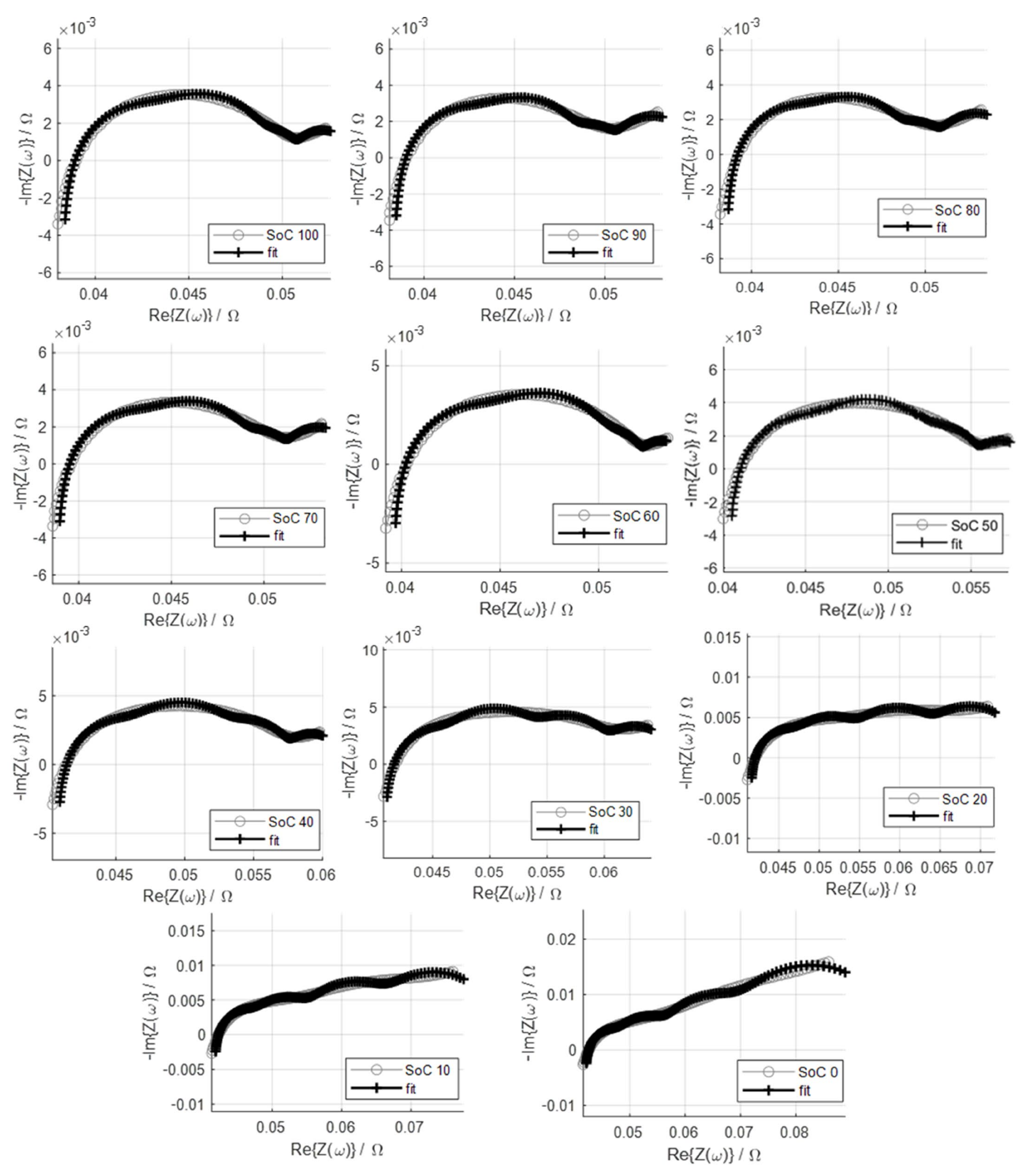
When these circuit elements are considered comprehensively, they exhibit similar properties to those in the battery cell operation process, but the individual physical properties cannot be explained in detail. Therefore, parameter values cannot be measured by laboratory test methods that separate specific physical properties. Instead, the optimization process allows the value of each element to be fitted so that the model prediction matches the measured cell data as well as possible. This process is called system identification. Measured impedance data are fitted to an equivalent circuit representing the physical processes occurring in the system. Fitting of the impedance spectrum must be performed on both the imaginary and the real parts of the data. This can be achieved by complex nonlinear least squares (CNLS) fitting. The fit accuracy is used to determine whether the proposed impedance model and the obtained fitting parameters are suitable for the purpose.

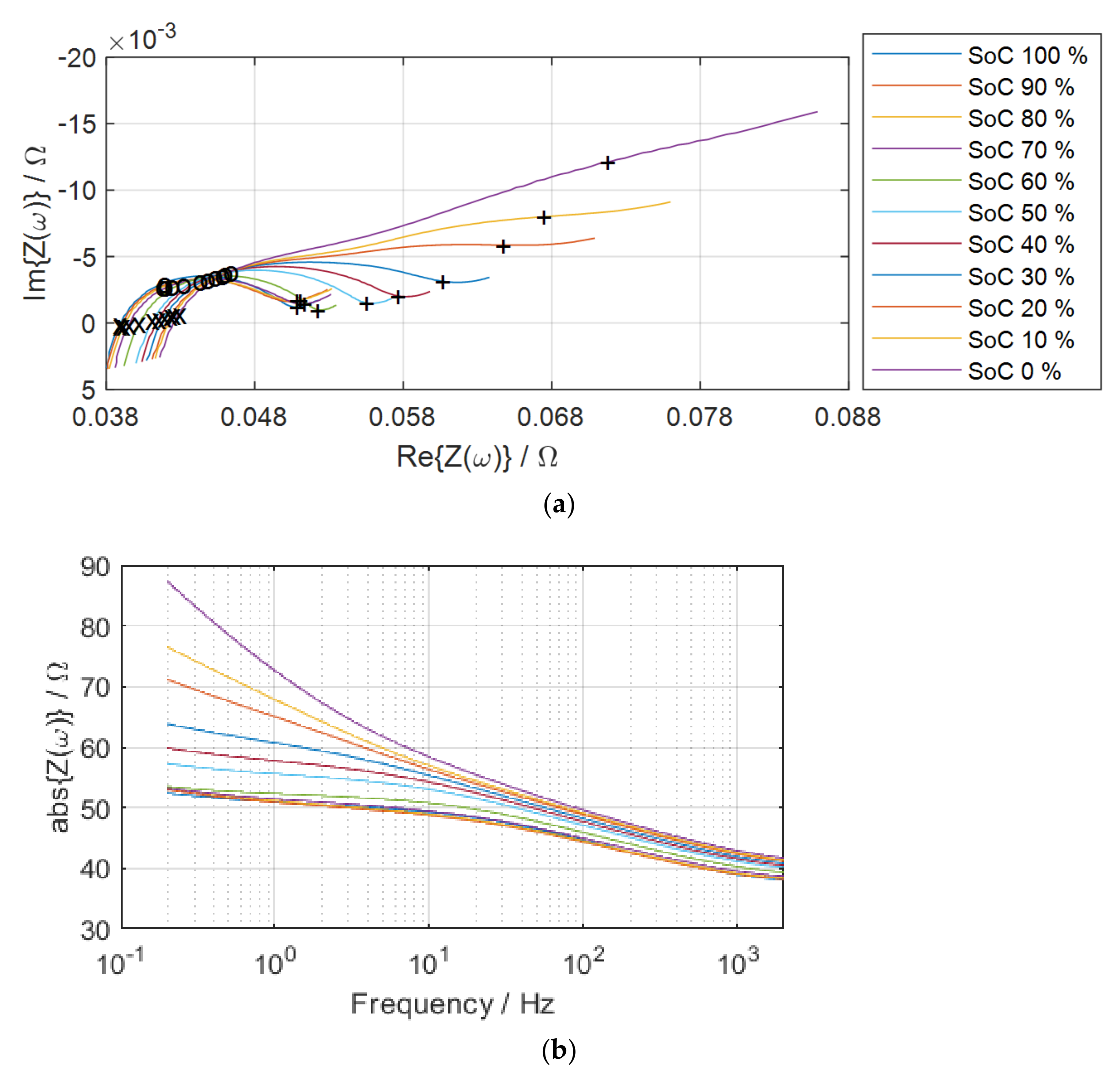
Electrochemical impedance spectroscopy (EIS) is a non-invasive analysis technique for measuring battery cell parameters that establish model structures due to cell SoC, SoH, aging, temperature, internal defects, etc. [28]. EIS is based on the fact that electrochemical loss processes occur over a wide range of frequencies [29], and as each process has its own time constant [30], EIS can isolate most of these processes [31]. EIS measurements are performed in a wide frequency range from several kHz to several mHz to obtain a characteristic impedance spectrum [32]. If multiple frequencies are applied simultaneously, this measurement time can be shortened, and this method is called multi-sine EIS [9].

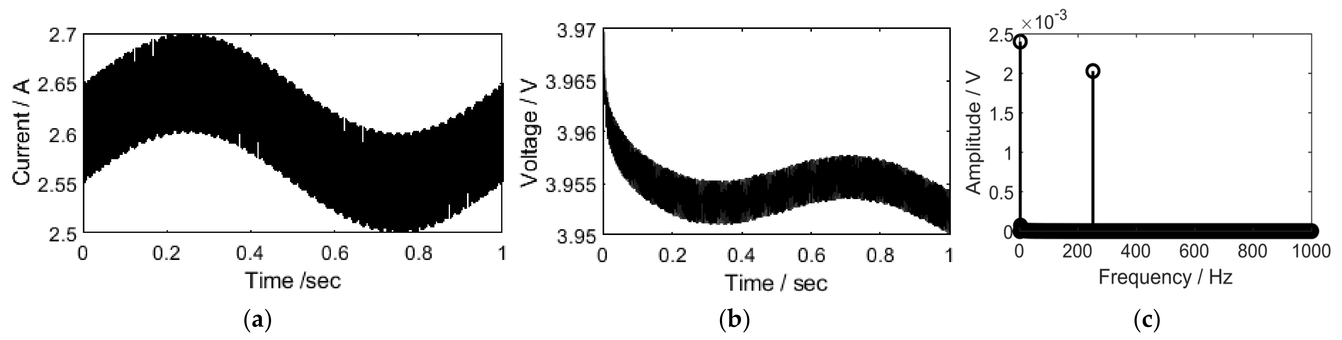
EIS measurements include applying small sinusoidal voltage or current signals to electrochemical cells and measuring system reactions in amplitude and phase (real and imaginary parts) to determine cell impedance. The complex impedance contains information on the amplitude and phase between the voltage and current signals for each different frequency. If the current $𝒾$ of the battery cell is given by Equation (1), and the voltage $ℯ$  is measured as Equation (2), the cell impedance Z can be obtained as Equation (3).

$$𝒾={\mathrm{I}}_{\mathrm{dc}}+{\mathsf{\Delta }\mathrm{I}}_{\mathrm{f}}·\sin \left(2\mathsf{\pi }\mathrm{ft}\right)$$

(1)

$$ℯ={\mathrm{E}}_{\mathrm{dc}}+{\mathsf{\Delta }\mathrm{E}}_{\mathrm{f}}·\sin \left(2\mathsf{\pi }\mathrm{ft}+{\mathsf{\varphi }}_{\mathrm{f}}\right)$$

(2)

$${\mathrm{Z}}_{\mathrm{f}}=\frac{{\mathsf{\Delta }\mathrm{E}}_{\mathrm{f}}}{{\mathsf{\Delta }\mathrm{I}}_{\mathrm{f}}}·{\mathrm{e}}^{\mathrm{j}{\mathsf{\varphi }}_{\mathrm{f}}}=\left|{\mathrm{Z}}_{\mathrm{f}}\right|·{\mathrm{e}}^{\mathrm{j}{\mathsf{\varphi }}_{\mathrm{f}}}={\mathrm{Z}}_{\mathrm{f}}^{\prime }+\mathrm{j}·{\mathrm{Z}}_{\mathrm{f}}^{″}$$

(3)

where ${\mathrm{I}}_{\mathrm{dc}}$ is direct current (DC) bias, ${\mathsf{\Delta }\mathrm{I}}_{\mathrm{f}}$ is the amplitude of the excited test frequency f, ${\mathrm{E}}_{\mathrm{dc}}$ is the offset voltage, ${\mathsf{\Delta }\mathrm{E}}_{\mathrm{f}}$ is the amplitude of the output voltage, and ${\mathsf{\varphi }}_{\mathrm{f}}$ is the phase difference.

As shown in Equation (3), the electrochemical impedance of a battery cell is a frequency-dependent complex number characterized by its modulus $\left|{\mathrm{Z}}_{\mathrm{f}}\right|$ and phase angle ${\mathrm{e}}^{\mathrm{j}\mathsf{\varphi }}$. Another expression is given as the real and imaginary parts of the complex impedance.

In this paper, an equivalent circuit model for Li-ion battery cells is developed in the MATLAB/Simulink environment. Therefore, the proposed model can be easily connected to other circuit blocks in MATLAB/Simulink. Each element value of the equivalent circuit model is determined by the EIS measured in different cell SoCs.

In Section 2, the proposed model is presented. Selection of model parameters and details of each simulation block are described. In Section 3, the model is validated with simulation results under various conditions compared to the measurement, and Section 4 deals with conclusion and discussions.

2. The Proposed Model

Figure 1 shows the overall appearance of the Matlab/Simulink model. The input current (${\mathrm{Current}}_{\mathrm{in}}$) is a signal obtained by adding two frequency signals (Test Freq. 1, Test Freq. 2) to the DC offset. The SoC model provides a real-time SoC to the cell model. The initial SoC is given as ${\mathrm{SoC}}_{\mathrm{init}}$, and the real-time SoC is output as ${\mathrm{SoC}}_{\mathrm{out}}$. The rate capacity effect is considered in this model. SoCs are calculated based on dischargeable cell capacity, which varies with operating current (C-rate) [33,34]. The SoC correction model is used to consider the rate capacity effect. The cell model receives a real-time SoC and current and outputs a real-time cell voltage (${\mathrm{V}}_{\mathrm{cell}}$). The output voltage ${\mathrm{V}}_{\mathrm{cell}}$ is Fourier transformed to calculate the cell impedance at each test frequency. Cell impedance calculations take into account cell SoH and cell temperature. The details of each subsystem are described in the following subsections. The doi address for downloading this Simulink model is provided at the end of this paper.

2.1. SoC Model

In this model, the cell SoC is represented by Equation (4). The output of this subsystem is a real-time SoC (${\mathrm{SoC}}_{\mathrm{out}}$):

$${\mathrm{SoC}}_{\mathrm{out}}={\mathrm{SoC}}_{\mathrm{init}}-\int \frac{{\mathrm{Current}}_{\mathrm{in}}\times 100}{\mathrm{Q}\times 3600}\mathrm{dt}$$

(4)

where Q is the nominal capacity (Ah) of the cell.

Figure 2 shows the voltage curves of the Li-ion battery cell discharged at different C-rates, and

Table 1. Specifications of the Li-ion battery cell.

Parameter	Description
Product name	Samsung ICR 18650-26F
Battery system	Li-ion
Nominal voltage	3.7 V
Rated capacity	2.6 Ah (0.2 C, to 2.75 V discharge)
Wh rating	9.62 Wh
Anode	Based on intercalation graphite
Cathode	Based on lithiated metal oxide 1

¹ Consists of cobalt, nickel, and manganese.

shows the specifications of the cell used for modeling.

Table 2. Relative capacities of a Li-ion battery cell discharged at different C-rates.

C-Rate	Relative Capacity
1.5	0.92
1	0.92
0.5	0.94
0.25	0.97
0.125	1

shows the relative capacity of the cell when discharged at different C-rates. The higher the C-rate, the less the total amount of energy (Wh) that can be released from the cell. If the usable capacity of the cell at 0.125 C is 100%, the usable relative capacity at 1.5 C is 92%.

This is implemented in the SoC correction model using a 2D lookup table that receives ${\mathrm{SoC}}_{\mathrm{out}}$ and ${\mathrm{Current}}_{\mathrm{in}}$ as inputs. The SoC output corrected by the discharge current is expressed as ${\mathrm{SoC}}_{\mathrm{c}}$.

2.2. Cell Model

Impedance between frequencies 1 Hz and 1 kHz is considered especially useful for estimating SoC and SoH of battery cells used in the model [8,9]. The equivalent circuit in Figure 3 is used considering the accuracy of fit and complexity of the model in the corresponding frequency range.

The ECM adopted in this model consists of a DC voltage source, an inductor, a series resistor, and four RC parallel networks. The DC voltage source is used to represent the open circuit voltage (OCV) of the cell, the series resistor (R0) is used to represent the internal DC resistance, and the RC parallel network (R1, C1, R2, C2, R3, C3, R4, C4) is used to characterize the transient response of voltage L, which represents the inductive behavior of the cell, increases the accuracy of the impedance fit at frequencies above ~1 kHz.

In the ECM represented by Figure 3, the cell output voltage (${\mathrm{V}}_{\mathrm{cell}}$) is calculated by Equation (5).

$${\mathrm{V}}_{\mathrm{cell}}=\mathrm{OCV}-{\mathrm{V}}_{\mathrm{L}}-{\mathrm{V}}_{\mathrm{R}0}-{\displaystyle \sum }_{\mathrm{n}=1}^4{\mathrm{V}}_{\mathrm{Pn}}$$

(5)

where ${\mathrm{V}}_{\mathrm{L}}$ is the inductor voltage, ${\mathrm{V}}_{\mathrm{R}0}$ is the series resistance voltage, and ${\mathrm{V}}_{\mathrm{Pn}}$ is the n-th RC parallel network voltage. Calculation of each voltage is described in subsequent subsections.

2.2.1. OCV Measurement and Application

OCV is the voltage of the battery cell at equilibrium. The value of OCV depends on the SoC. In this paper, cell OCV is measured through the following procedure:

• Constant current (CC) charge: The cell is charged with a 1 C current until a high cut-off voltage (4.2 V) is reached.
• Constant voltage (CV) charge: When the cell reaches a voltage of 4.2 V, the charging current is reduced to maintain the voltage. Charging is terminated when the current becomes 1/10 C.
• Ninety minutes of relaxation is given to the cell. This step completes setting cell SoC to 100%.
• Discharge of 1 C for 5 min and relaxation for 10 min are repeated. The cell voltage at this time is shown by the solid line in Figure 4.
• When the cell voltage reaches a low cut-off voltage (2.8 V), the discharge is terminated and a final relaxation time of 10 min is given. At this step, the SoC of the cell becomes 0%.
• The cell voltage after each 10 min relaxation is collected as an OCV voltage. In Figure 4, the measured OCV is shown by the round marker.

This series of procedures is performed in a cell in the temperature chamber of BINDER GmbH set to 25 °C.

Cell OCV is applied to the model as a lookup table that receives SoC as input.

2.2.2. System Identification and Calculation of Cell Voltage

The elements of the equivalent circuit in Figure 3 depend on the cell SoC. EIS equipment (IM6ex from Zahner-Elektrik GmbH & CoKG) is used to measure cell impedance at each SoC in a temperature chamber set to 25 °C.

Table 3. Parameters for EIS measurement.

Parameter	Description
EIS method	Galvanostatic
Min. frequency	200 mHz
Max. frequency	2 kHz
DC bias	0 A
AC amplitude	100 mA

shows the parameters used for the EIS measurement.

Figure 5 shows the cell impedance in each cell SoC at 95% SoH in Nyquist plots (a) and Bode plots (b). The cell impedance of cell SoC at each 10% from 100% to 0% is shown.

The lower the cell SoC, the higher the cell impedance. In addition, the lower the frequency, the higher the cell impedance. Lower frequencies result in greater impedance differences for each SoC, making it advantageous for low frequency impedance to be used to distinguish each cell SoC. However, the lower the frequency, the longer the period required to measure the impedance. The 1 Hz impedance can be used to estimate the impedance for cell SoC estimation every second [9].

The cell impedance whose imaginary part becomes 0 represents the series resistance of the cell and can be used to estimate the cell SoH. As a result of the measurement, the imaginary part of the impedance at ~1 kHz approaches zero, so it is suitable for use in cell SoH estimation. However, impedance at lower frequencies may be used depending on hardware performance and the required estimation accuracy. For example, 250 Hz impedance is used for SoH estimation in [8].

The cell impedance in Figure 5 is fitted to each element of the cell equivalent circuit. For the fitting of equivalent circuit elements, an algorithm to find the minimum χ² value is used. χ² calculates the distance between measured and simulated data, defined as Equation (6).

$$\begin{array}{c}{\mathsf{\chi }}^2=\sum _{\mathrm{i}=1}^{\mathrm{n}}{\left|{\mathrm{Z}}_{\mathrm{meas}}\left(\mathrm{i}\right)-{\mathrm{Z}}_{\mathrm{simul}}\left({\mathrm{f}}_{\mathrm{i}},\mathrm{element}\right)\right|}^2=\sum \{\frac{{\left(\mathrm{Re}\left({\mathrm{Z}}_{\mathrm{simul}}\right)-\mathrm{Re}\left({\mathrm{Z}}_{\mathrm{meas}}\right)\right)}^2}{{\left(\mathrm{Re}\left({\mathrm{Z}}_{\mathrm{meas}}\right)\right)}^2}+\\ \frac{{\left(\mathrm{Im}\left({\mathrm{Z}}_{\mathrm{simul}}\right)-\mathrm{Im}\left({\mathrm{Z}}_{\mathrm{meas}}\right)\right)}^2}{{\left(\mathrm{Im}\left({\mathrm{Z}}_{\mathrm{meas}}\right)\right)}^2}\}\end{array}$$

(6)

where ${\mathrm{Z}}_{\mathrm{meas}}\left(\mathrm{i}\right)$ is the measured impedance at the frequency ${\mathrm{f}}_{\mathrm{i}}$, ${\mathrm{Z}}_{\mathrm{simul}}\left({\mathrm{f}}_{\mathrm{i}},\mathrm{parameter}\right)$ is a function of the chosen model, and element is the model element.

A lower ${\mathsf{\chi }}^2$ indicates a higher fit accuracy, and thus this should be minimized. ${\mathsf{\chi }}^2$/N with N points is the normalized expression of ${\mathsf{\chi }}^2$, whose value is independent of the number of points and represents the error.

Table 4. Fitted element values for each SoC and ${\mathsf{\chi }}^2/N$ representing the fitting error.

SoC (%)	${\mathit{\chi }}^2/\mathit{N}$	L (H)	R0 (Ω)	R1 (Ω)	C1 (F)	R2 (Ω)	C2 (F)	R3 (Ω)	C3 (F)	R4 (Ω)	C4 (F)
100	1.77 × 10−3	3.41 × 10−7	3.82 × 10−2	1.81 × 10−3	1.75 × 10	5.53 × 10−3	5.38 × 10−1	5.23 × 10−3	7.82 × 10−2	3.01 × 10−3	2.16 × 102
90	1.98 × 10−3	3.38 × 10−7	3.83 × 10−2	2.24 × 10−3	1.67 × 10	5.12 × 10−3	6.10 × 10−1	4.98 × 10−3	8.36 × 10−2	4.30 × 10−3	1.55 × 102
80	2.12 × 10−3	3.36 × 10−7	3.85 × 10−2	2.32 × 10−3	1.57 × 10	5.06 × 10−3	6.22 × 10−1	5.02 × 10−3	8.33 × 10−2	4.41 × 10−3	1.48 × 102
70	2.06 × 10−3	3.33 × 10−7	3.88 × 10−2	2.17 × 10−3	1.57 × 10	5.23 × 10−3	5.92 × 10−1	5.03 × 10−3	8.09 × 10−2	3.69 × 10−3	1.88 × 102
60	2.05 × 10−3	3.27 × 10−7	3.95 × 10−2	1.81 × 10−3	1.67 × 10	5.70 × 10−3	5.47 × 10−1	5.19 × 10−3	7.78 × 10−2	2.20 × 10−3	3.24 × 102
50	2.37 × 10−3	3.25 × 10−7	4.03 × 10−2	3.17 × 10−3	8.79	6.58 × 10−3	4.80 × 10−1	5.38 × 10−3	7.00 × 10−2	3.02 × 10−3	2.05 × 102
40	2.32 × 10−3	3.20 × 10−7	4.07 × 10−2	4.25 × 10−3	7.03	6.96 × 10−3	4.82 × 10−1	5.62 × 10−3	6.80 × 10−2	3.93 × 10−3	1.54 × 102
30	3.02 × 10−3	3.48 × 10−7	4.07 × 10−2	6.30 × 10−3	5.42	7.59 × 10−3	4.27 × 10−1	5.72 × 10−3	5.75 × 10−2	5.76 × 10−3	9.97 × 10
20	2.41 × 10−3	3.05 × 10−7	4.14 × 10−2	9.32 × 10−3	4.39	7.39 × 10−3	4.80 × 10−1	5.99 × 10−3	6.52 × 10−2	1.11 × 10−2	4.73 × 10
10	2.37 × 10−3	3.01 × 10−7	4.16 × 10−2	1.12 × 10−2	4.01	7.64 × 10−3	4.75 × 10−1	6.10 × 10−3	6.46 × 10−2	1.59 × 10−2	3.32 × 10
0	2.45 × 10−3	2.99 × 10−7	4.19 × 10−2	1.35 × 10−2	3.51	8.50 × 10−3	4.46 × 10−1	6.16 × 10−3	6.26 × 10−2	2.81 × 10−2	1.98 × 10

shows the fitted equivalent circuit element values and the error ${\mathsf{\chi }}^2$/N in each SoC. Figure 6 shows the measured cell impedance and fitted results for each SoC as a Nyquist plot.

The fitted equivalent circuit element values in each SoC are respectively applied to the cell model as a lookup table.

The series inductor voltage (${\mathrm{V}}_{\mathrm{L}}$) is expressed as Equation (7) when the s-domain is used.

$${\mathrm{V}}_{\mathrm{L}}=\mathrm{L}\frac{\mathrm{di}}{\mathrm{dt}}=\mathrm{sLI}$$

(7)

The series resistance voltage (${\mathrm{V}}_{\mathrm{R}0}$) of the equivalent circuit is expressed by Equation (8).

$${\mathrm{V}}_{\mathrm{R}0}=\mathrm{I}\times \mathrm{R}0$$

(8)

By using s-domain, the voltage of n-th RC parallel network (${\mathrm{V}}_{\mathrm{Pn}}$) can be expressed as Equation (9).

$${\mathrm{V}}_{\mathrm{Pn}}=\left(\frac{1}{\mathrm{s}}\right)\left[\frac{\mathrm{I}}{\mathrm{C}}-\frac{\mathrm{V}}{\mathrm{RC}}\right]$$

(9)

When Equations (7)–(9) are used with the OCV obtained in Section 2.2.1, the cell voltage (${\mathrm{V}}_{\mathrm{Cell}}$) can be calculated as Equation (5).

2.3. Output of Continuous Cell Impedance

The cell voltage output (${\mathrm{V}}_{\mathrm{Cell}}$) from the cell model is Fourier transformed in a callback function called StopFcn to obtain the amplitude of the output voltage at each test frequency. If amplitudes at frequencies up to 1 kHz are to be measured, a sampling rate of at least 2 kHz should be used to satisfy the Nyquist–Shannon sampling theory. In addition, the number of data for the Fourier transform must be the n-th power of 2. In the simulation, a sampling rate of 2048 Hz is used, which samples 2048 ($=2^{11}$) voltage data every second. The sample time of each test frequency generation model is set to ‘1/sampling rate’. The step size in the ‘model solver’ should also be an expression related to the sampling rate. ‘1/sampling rate’ is used for the ‘max step size’. Figure 7a shows the input current (${\mathrm{Current}}_{\mathrm{in}}$) for 1 s, and Figure 7b shows the output voltage for 1 s (${\mathrm{Voltage}}_{\mathrm{out}}$). If the voltage data in the time domain of Figure 7b are Fourier transformed, they can be expressed in the frequency domain as shown in Figure 7c.

The output voltage amplitudes at 1 Hz and 250 Hz obtained in Figure 7c are used to calculate the impedance at each frequency through Equation (3).

Figure 8 shows the impedance simulation results at 1 Hz, 10 Hz, 100 Hz, and 1 kHz of the cell during discharge. Here, cell depth of discharge (DoD) is defined as (100-SoC (%)) as the opposite concept of SoC. While the cell is discharged, the lower the frequency, the more impedance changes. This is consistent with the tendency shown in Figure 5.

Table 5. Increased rates in impedance at each frequency.

Frequency	Increased Rate
1 Hz	113.15%
10 Hz	107.29%
100 Hz	104.73%
1 kHz	104.32%

shows the rate of increase in impedance as cell DoD increases. The increase rate of cell impedance at 10 Hz, 100 Hz, and 1 kHz is calculated over the entire DoD range, but at 1 Hz, it is calculated in the 1% to 96% DoD range. This is to exclude impedance that is not properly measured [9].

2.4. Cell Temperature Model

At lower frequencies, impedance is more affected by cell temperature and cell SoC [8,9]. Figure 9 shows the temperature change of the cells discharged at each C-rate. Cell temperature is related to discharge current and discharge time. The temperature model is implemented as a 2D lookup table that receives the discharge current and discharge time as inputs, as shown in Figure 1.

The equation between cell temperature and cell impedance can be obtained from the empirical relationship through EIS measurement, which can be used to estimate impedance changes due to temperature changes [9]. The output ${\mathrm{T}}_{\mathrm{cell}}$ of the temperature model is used to adjust the impedance considering the temperature. The 1 Hz impedance ($\mathrm{Z}{\left(1\right)}_{\mathrm{model}}$) is adjusted to the cell temperature with Equation (10) and calculated as $\mathrm{Z}{\left(1\right)}_{\mathrm{adj}}$.

$$\mathrm{Z}{\left(1\right)}_{\mathrm{adj}}=\mathrm{Z}{\left(1\right)}_{\mathrm{model}}+0.066·{\mathrm{T}}_{\mathrm{cell}}^2-5.362·{\mathrm{T}}_{\mathrm{cell}}+93.52$$

(10)

3. Simulation Results and Validation

The simulation results are verified by comparing them with the measurement results. The test current, which is the sum of the two test frequency signals and the DC offset, is applied to the electronic load connected to the cell. USB-6212, which is the National Instruments’ Data Acquisition (DAQ) module, is used to input and output signals. The cell temperature is measured with NXP’s silicon temperature sensor KTY 81-110 attached to the cell surface. The detailed experimental setup for measuring the impedance of cells during discharging, including the circuit diagram of the electronic load, is covered in [8].

3.1. Simulation of Continuous Cell Impedance during Discharge

3.1.1. 1 Hz Impedance during Discharge

Table 6. Conditions for both simulation and measurement of the impedance of the cell during discharge.

Parameter	Description
DC offset	1.5 C, 1 C, 0.5 C, 0.25 C and 0.125 C
SoC	From 100% to 0%
Test frequency	1 Hz, 250 Hz
Amplitude	50 mA (each)

shows the parameters used for measurements and simulations. The 1 Hz impedance of a cell discharging at different C-rates is shown in Figure 10a. The measured impedance is represented by dotted lines and the simulation results by solid lines. Figure 10b shows the percentage error between the measured impedance and the simulation results.

Table 7. Average values of each percent error at different C-rates.

C-Rate	Percent Error (%)
1.5	2.28
1	2.36
0.5	1.32
0.25	0.76
0.125	0.56
Total	1.46

shows the mean of percentage errors at each C-rate.

3.1.2. 250 Hz Impedance at Each Cell SoH

Cell impedance can be used for cell SoH estimation. It is recommended that higher frequencies be used to be less affected by the SoC (Figure 5). For SoH estimation of cells, 250 Hz impedance is used in [8]. When a higher frequency of 1 kHz impedance is used for cell SoH estimation, the estimation error is slightly reduced compared to when 250 Hz is used, but higher hardware performance is required for data sampling [9]. In this paper, assuming that 250 Hz impedance is used for SoH estimation, Equation (11) for impedance adjustment according to SoH is applied to 250 Hz impedance in the simulation model [8].

$$\mathrm{Z}{\left(250\right)}_{\mathrm{adj}}=-0.1064·\mathrm{SoH}+54.8584$$

(11)

The results are shown in Figure 11, and the percentage errors compared to those measured in cells at each SoH are shown in

Table 8. Average values of percent errors of the estimated impedance relative to the measured impedance at different SoHs.

SoH (%)	Percent Error (%)
100	0.43
95	0.33
90	0.75
85	0.55
80	0.45
75	0.35
Mean	0.48

.

3.2. Simulation of Cell Impedance Discharging from Different Initial SoCs

In the preceding subsections, the simulation results are represented until the fully charged cell is completely discharged. However, the cell does not always discharge at 100% SoC. In this subsection, simulation results when cells are discharged at different initial SoCs are compared with measurement results. The experimental conditions are shown in

Table 9. Conditions for both simulation and measurement of impedance of a cell discharged from different initial SoCs.

Parameter	Description
Test frequency	1 Hz
Amplitude	50 mA
$\mathrm{DC}\mathrm{bias}({\mathrm{I}}_{\mathrm{d}\mathrm{c}}$)	2.6 A (1 C)
Depth of discharge	From 0 to 100%
Discharge time	10 min. (each)
Relaxation time	60 min. (each)
SoH	95%
Initial temperature	25 °C

. The cell is discharged for 10 min after a relaxation of 60 min. Then, 10 min of cell discharge and 60 min of cell relaxation are repeated until the cell is completely discharged. The cell impedance is measured every second while the cell is discharged.

Figure 12a shows the measured cell voltage (dotted line) and the model output voltage (solid line), and Figure 12b shows the percentage error between the measured voltage and the simulation result. The average of percent errors in the total DoD range is 0.42%.

Figure 13a shows the output of the cell temperature model. The cell temperature increases every 10 min of discharge, and after every 60 min of relaxation, the cell temperature decreases to 25 °C. Figure 13b shows the measured 1 Hz impedance (blue dotted line), simulated 1 Hz impedance (red solid line), and simulated 1 Hz cell impedance after being adjusted to temperature (green solid line). Figure 13c shows the percentage error between the measured 1 Hz impedance and the simulated 1 Hz impedance adjusted to temperature. The average percent error in the overall DoD is 2.59%, and the average percent error in DoD 0% to 95% is 1.16%.

3.3. Simulation Results at Different Diagnostic Parameters

The accuracy of the proposed simulation model is shown above compared to the measured results. As mentioned earlier, one of the advantages of this simulation model is that it shortens the time required for experiments. To show examples of use of this model, the following subsections compare simulation results of continuous cell impedance at different diagnostic parameters.

3.3.1. Simulation of Continuous Cell Impedance from 1 to 100 Hz

Figure 14a shows the cell impedance from 1 Hz to 100 Hz of cells discharging from DoD 0% to 100%. Figure 14b shows the increased rate of impedance in the range between 1% and 95% of DoD at each frequency. Impedance at each frequency is simulated at 1 Hz intervals. The simulation conditions are shown in

Table 10. Simulation conditions for comparing cell impedance from 1 Hz to 100 Hz.

Parameter	Description
Test frequency	1 Hz to 100 Hz
Depth of discharge	From 0 to 100%
SoH	95%
$\mathrm{DC}\mathrm{bias}({\mathrm{I}}_{\mathrm{d}\mathrm{c}}$)	1.3 A (0.5 C)
Sampling rate	2048 Hz
Amplitude	50 mA (each)

.

Figure 14a,b shows that the higher the frequency, the less impedance changes due to DoD changes, as shown in Figure 5. For this simulation to be measured as an experiment, it would take ~550 h (~23 days), assuming that the required time for temperature setting is excluded and cell SoH is not changed even in charging/discharging cycles (~120 min for CC-CV charging + 90 min for relaxation + ~120 min for 0.5 C discharge) × 100 times).

3.3.2. Simulation of Continuous Cell Impedance at Different Sampling Rates

Figure 15a shows the simulation results of cell impedance during discharge at different sampling rates. Figure 15b shows the percentage error of simulation results at sampling rate 2048 Hz and from 16 Hz to 1024 Hz.

Table 11. Simulation conditions for comparing continuous 1 Hz impedance at different sampling rates.

Parameter	Description
Sampling rate	16 Hz to 2048 Hz
Test frequency	1 Hz
Depth of discharge	From 0 to 100%
SoH	95%
$\mathrm{DC}\mathrm{bias}({\mathrm{I}}_{\mathrm{d}\mathrm{c}}$)	1.3 A (0.5 C)
Amplitude	50 mA (each)

shows the simulation conditions.

Figure 15 shows that the lower the sampling rate, the lower the output impedance. This does not mean that the cell impedance actually decreased, but that the measurement error increased. In Fourier transformations, the lower sampling rate results in fewer samples collected in one cycle of signals in the time domain, resulting in a greater error due to the failure of the signal to restore properly in the frequency domain.

Table 12. Percent errors of the mean of the impedance simulated at a sampling rate of 2048 Hz and the mean of the impedance simulated at each different sampling rate.

Sampling Rate	Percent Error
16 Hz	1.63%
32 Hz	0.48%
64 Hz	0.16%
128 Hz	0.06%
256 Hz	0.026%
512 Hz	0.01%
1024 Hz	0.00%
2048 Hz	Reference

shows the average of the percent errors at each sampling rate in Figure 15b.

As shown in Table 12, when a sampling rate of 16 Hz is used, an average error of 1.63% occurs compared to when 2048 Hz is used. Meanwhile, the simulation result when a sampling rate of 1024 Hz is used does not reveal the difference from when 2048 Hz is used. Such information can be used to select diagnostic parameters and hardware performance for optimized cell monitoring.

4. Conclusions and Discussion

The aim of this paper is to propose a model for optimization and simulation of cell SoC and cell SoH monitoring algorithms of lithium-ion battery cells. In particular, the output cell voltage and the subsequent continuous cell impedance are successfully predicted when multiple frequency signals are applied to the cell operation DC bias. In addition, the proposed model also successfully predicts cell-continuous impedance when cells are discharged at different initial SoCs. The effects of cell SoC, cell SoH, cell temperature, and C-rate are considered on the output impedance in this model. Moreover, examples show that the proposed simulation model is used to optimize the parameters of the cell state monitoring algorithm.

The proposed model can be used not only to save the cost of building an experimental system, but also to quickly obtain output from the input of each state parameter, saving time to prepare for each cell state. The simulation of cell behavior in various situations over a short period of time saves time in selecting optimal state estimation parameters using the cell impedance before starting the experiment.

Nevertheless, the following factors should be noted:

• As shown in Figure 10 and Figure 13, the estimation error of cell impedance gradually increases at DoD above about 90%. This is a problem due to the characteristics of the Li-ion battery cells. When the DoD of the cell increases above a certain level, the cell voltage decreases significantly nonlinearly, resulting in a large error in impedance measurement as shown in Figure 12. In addition, when estimating the cell voltage, the estimation error is relatively higher in the early stages of the discharge when the cell voltage is nonlinearly lowered. Despite the characteristics of Li-ion cells with this nonlinearity, this model shows competent overall estimation results.
• This model estimates the cell voltage and impedance only during discharge, not during charging. In the reference, to estimate the cell SoH, both cell impedance during discharge and charging are compared. Reference [9] only uses cell impedance while discharging to estimate cell SoC and mentions the difficulty of using impedance while charging. This model focuses on monitoring the cell state with impedance during discharge. Nevertheless, it is clear that application in a wider range will be possible when the proposed model can also estimate cell voltage and impedance during charging through further research.
• Last, cells are discharged in a temperature chamber adjusted to 25 °C in this paper. Therefore, the cell temperature is only considered from 25 to 30 °C. For wider conditions to be considered, the temperature range of the model will be increased.

References

1. Da Silva, S.P.; Da Silva, P.R.C.; Urbano, A.; Scarminio, J. Analysis of a commercial portable lithium-ion battery under low current charge-discharge cycles. Química Nova 2016, 39, 901–905. [Google Scholar] [CrossRef]
2. Rajaeifar, M.A.; Ghadimi, P.; Raugei, M.; Wu, Y.; Heidrich, O. Challenges and recent developments in supply and value chains of electric vehicle batteries: A sustainability perspective. Resour. Conserv. Recycl. 2022, 180, 106144. [Google Scholar] [CrossRef]
3. Bruce, G.; Mardikian, P.; Marcoux, L. 50 to 100 Ah lithium-ion cells for aircraft and spacecraft applications. J. Power Sources 1997, 65, 149–153. [Google Scholar] [CrossRef]
4. Mousavi G., S.M. An autonomous hybrid energy system of wind/tidal/microturbine/battery storage. Int. J. Electr. Power Energy Syst. 2012, 43, 1144–1154. [Google Scholar] [CrossRef]
5. Zhou, Z.; Benbouzid, M.; Frédéric Charpentier, J.; Scuiller, F.; Tang, T. A review of energy storage technologies for marine current energy systems. Renew. Sustain. Energy Rev. 2013, 18, 390–400. [Google Scholar] [CrossRef] [Green Version]
6. Majima, M.; Ujiie, S.; Yagasaki, E.; Koyama, K.; Inazawa, S. Development of long life lithium ion battery for power storage. J. Power Sources 2001, 101, 53–59. [Google Scholar] [CrossRef]
7. Doughty, D.H.; Roth, E.P. A General Discussion of Li Ion Battery Safety. Electrochem. Soc. Interface 2012, 37. [Google Scholar] [CrossRef] [Green Version]
8. Kim, J.; Krüger, L.; Kowal, J. On-line state-of-health estimation of Lithium-ion battery cells using frequency excitation. J. Energy Storage 2020, 32, 101841. [Google Scholar] [CrossRef]
9. Kim, J.; Kowal, J. A Method for Monitoring State-of-Charge of Lithium-Ion Cells Using Multi-Sine Signal Excitation. Batteries 2021, 7, 76. [Google Scholar] [CrossRef]
10. Zhang, Q.; Wang, D.; Yang, B.; Cui, X.; Li, X. Electrochemical model of lithium-ion battery for wide frequency range applications. Electrochim. Acta 2020, 343, 136094. [Google Scholar] [CrossRef]
11. Rahman, M.A.; Anwar, S.; Izadian, A. Electrochemical model parameter identification of a lithium-ion battery using particle swarm optimization method. J. Power Sources 2016, 307, 86–97. [Google Scholar] [CrossRef]
12. Sung, W.; Shin, C.B. Electrochemical model of a lithium-ion battery implemented into an automotive battery management system. Comput. Chem. Eng. 2015, 76, 87–97. [Google Scholar] [CrossRef]
13. Smith, K.A.; Rahn, C.D.; Wang, C.-Y. Control oriented 1D electrochemical model of lithium ion battery. Energy Convers. Manag. 2007, 48, 2565–2578. [Google Scholar] [CrossRef]
14. Rahul, K.; Ramprabhakar, J.; Shankar, S. Comparative study on modeling and estimation of State of Charge in battery. In Proceedings of the 2017 International Conference on Smart Technologies for Smart Nation (SmartTechCon), Bangalore, India, 17–19 August 2017; IEEE: Piscataway, NJ, USA, 2017; pp. 1610–1615, ISBN 978-1-5386-0569-1. [Google Scholar]
15. Wei, J.; Dong, G.; Chen, Z. Remaining Useful Life Prediction and State of Health Diagnosis for Lithium-Ion Batteries Using Particle Filter and Support Vector Regression. IEEE Trans. Ind. Electron. 2018, 65, 5634–5643. [Google Scholar] [CrossRef]
16. Chen, L.; Wang, Z.; Lu, Z.; Li, J.; Ji, B.; Wei, H.; Pan, H. A Novel State-of-Charge Estimation Method of Lithium-Ion Batteries Combining the Grey Model and Genetic Algorithms. IEEE Trans. Power Electron. 2018, 33, 8797–8807. [Google Scholar] [CrossRef] [Green Version]
17. Zhang, C.; Zhu, Y.; Dong, G.; Wei, J. Data-driven lithium-ion battery states estimation using neural networks and particle filtering. Int. J. Energy Res. 2019, 43, 8230–8241. [Google Scholar] [CrossRef]
18. Bao, Y.; Dong, W.; Wang, D. Online Internal Resistance Measurement Application in Lithium Ion Battery Capacity and State of Charge Estimation. Energies 2018, 11, 1073. [Google Scholar] [CrossRef] [Green Version]
19. Randles, J.E.B. Kinetics of rapid electrode reactions. Discuss. Faraday Soc. 1947, 1, 11. [Google Scholar] [CrossRef]
20. Randles, J.E.B. Kinetics of rapid electrode reactions. Part 2. Rate constants and activation energies of electrode reactions. Trans. Faraday Soc. 1952, 48, 828–832. [Google Scholar] [CrossRef]
21. Randles, J.E.B.; Somerton, K.W. Kinetics of rapid electrode reactions. Part 3. Electron exchange reactions. Trans. Faraday Soc. 1952, 48, 937–950. [Google Scholar] [CrossRef]
22. Xia, B.; Sun, Z.; Zhang, R.; Lao, Z. A Cubature Particle Filter Algorithm to Estimate the State of the Charge of Lithium-Ion Batteries Based on a Second-Order Equivalent Circuit Model. Energies 2017, 10, 457. [Google Scholar] [CrossRef] [Green Version]
23. Wang, Y.; Liu, C.; Pan, R.; Chen, Z. Modeling and state-of-charge prediction of lithium-ion battery and ultracapacitor hybrids with a co-estimator. Energy 2017, 121, 739–750. [Google Scholar] [CrossRef]
24. Zhang, X.; Lu, J.; Yuan, S.; Yang, J.; Zhou, X. A novel method for identification of lithium-ion battery equivalent circuit model parameters considering electrochemical properties. J. Power Sources 2017, 345, 21–29. [Google Scholar] [CrossRef]
25. Hu, X.; Yuan, H.; Zou, C.; Li, Z.; Zhang, L. Co-Estimation of State of Charge and State of Health for Lithium-Ion Batteries Based on Fractional-Order Calculus. IEEE Trans. Veh. Technol. 2018, 67, 10319–10329. [Google Scholar] [CrossRef]
26. Tian, J.; Xiong, R.; Yu, Q. Fractional-Order Model-Based Incremental Capacity Analysis for Degradation State Recognition of Lithium-Ion Batteries. IEEE Trans. Ind. Electron. 2019, 66, 1576–1584. [Google Scholar] [CrossRef]
27. Wang, Y.; Gao, G.; Li, X.; Chen, Z. A fractional-order model-based state estimation approach for lithium-ion battery and ultra-capacitor hybrid power source system considering load trajectory. J. Power Sources 2020, 449, 227543. [Google Scholar] [CrossRef]
28. Gao, P.; Zhang, C.; Wen, G. Equivalent circuit model analysis on electrochemical impedance spectroscopy of lithium metal batteries. J. Power Sources 2015, 294, 67–74. [Google Scholar] [CrossRef]
29. Momma, T.; Matsunaga, M.; Mukoyama, D.; Osaka, T. Ac impedance analysis of lithium ion battery under temperature control. J. Power Sources 2012, 216, 304–307. [Google Scholar] [CrossRef]
30. Illig, J.; Schmidt, J.P.; Weiss, M.; Weber, A.; Ivers-Tiffée, E. Understanding the impedance spectrum of 18650 LiFePO4-cells. J. Power Sources 2013, 239, 670–679. [Google Scholar] [CrossRef]
31. Schmidt, J.P.; Chrobak, T.; Ender, M.; Illig, J.; Klotz, D.; Ivers-Tiffée, E. Studies on LiFePO4 as cathode material using impedance spectroscopy. J. Power Sources 2011, 196, 5342–5348. [Google Scholar] [CrossRef]
32. Osaka, T.; Mukoyama, D.; Nara, H. Review—Development of Diagnostic Process for Commercially Available Batteries, Especially Lithium Ion Battery, by Electrochemical Impedance Spectroscopy. J. Electrochem. Soc. 2015, 162, A2529–A2537. [Google Scholar] [CrossRef]
33. Jongerden, M.R.; Haverkort, B.R. Which battery model to use? IET Softw. 2009, 3, 445. [Google Scholar] [CrossRef] [Green Version]
34. Rao, R.; Vrudhula, S.; Rakhmatov, D.N. Battery modeling for energy-aware system design. Computer 2003, 36, 77–87. [Google Scholar] [CrossRef]
Figure 1. Overall view of the proposed simulation model.
Batteries 08 00008 g001
Figure 2. Voltage curves of the Li-ion battery cell discharged at different C-rates.
Batteries 08 00008 g002
Figure 3. Cell equivalent circuit used in the model.
Batteries 08 00008 g003
Figure 4. OCV of the battery cell used for modeling.
Batteries 08 00008 g004
Figure 5. Nyquist plots (a) and Bode plots (b) showing impedance at each cell SoC. In the Nyquist plot, the ‘+’ marker represents 1 Hz impedance, the ‘o’ marker represents 250 Hz impedance, and the ‘x’ marker represents 1 kHz impedance.
Batteries 08 00008 g005
Figure 6. Nyquist plots of measured cell impedance and fitted results.
Batteries 08 00008 g006
Figure 7. Input current (a) and output voltage (b) expressed in the time domain, and the output voltage expressed in the frequency domain (c) as a result of the simulation model.
Batteries 08 00008 g007
Figure 8. Simulation results of 1, 10, 100, and 1000 Hz impedance in the entire DoD range of the discharged cell.
Batteries 08 00008 g008
Figure 9. Temperature changes of cells discharging at different C-rates.
Batteries 08 00008 g009
Figure 10. (a) Simulated and measured 1 Hz impedance of cells discharged at different C-rates (dashed line: measured impedance; solid line: simulated impedance). (b) Percentage errors of the estimated impedance compared to the measured impedance at different C-rates.
Batteries 08 00008 g010
Figure 11. Continuous 250 Hz impedance at each SoH (dashed line: measured impedance, solid line: simulated impedance).
Batteries 08 00008 g011
Figure 12. (a) Discharge curve of a cell in which 10 min of discharge and 60 min of relaxation are repeated (dashed line: measured voltage, solid line: simulated voltage). (b) Percentage error of simulated cell voltage compared to the measured voltage.
Batteries 08 00008 g012
Figure 13. (a) Output of the cell temperature model when discharging for 10 min and relaxation for 60 min are repeated. (b) Measured continuous 1 Hz impedance and simulated results (red line: before adjusting to temperature; green line: after adjusting to temperature). (c) Percent error of simulated 1 Hz impedance considering the cell temperature compared to the measured impedance.
Batteries 08 00008 g013aBatteries 08 00008 g013b
Figure 14. (a) Continuous cell impedance from 1 Hz to 100 Hz simulated in the entire DoD range. (b) The increased rate of impedance at each frequency.
Batteries 08 00008 g014
Figure 15. (a) Continuous cell impedance in the entire DoD range simulated at different sampling rates. (b) Percentage errors of the simulation results between at the sampling rate of 2048 Hz and at each sampling rate of 16 Hz to 1024 Hz.
Batteries 08 00008 g015