Article

Physics-Informed Recurrent Neural Networks with Fractional-Order Constraints for the State Estimation of Lithium-Ion Batteries

1
School of Vehicle and Mobility, Tsinghua University, Beijing 100084, China
2
Department of Engineering, University of California, Merced, CA 95343, USA
*
Authors to whom correspondence should be addressed.
Batteries 2022, 8(10), 148; https://doi.org/10.3390/batteries8100148
Submission received: 17 August 2022 / Revised: 7 September 2022 / Accepted: 21 September 2022 / Published: 1 October 2022
(This article belongs to the Collection Advances in Battery Energy Storage and Applications)

Abstract

:
The state estimation of lithium-ion battery is the basis of an intelligent battery management system; therefore, both model-based and data-driven methods have been designed and developed for state estimation. Rather than using complex partial differential equations and the complicated parameter tuning of a model-based method, a machine learning algorithm provides a new paradigm and has been increasingly applied to cloud big-data platforms. Although promising, it is now recognized that big data for machine learning may not be consistent in terms of data quality with reliable labels. Moreover, many algorithms are still applied as a black box that may not learn battery inner information well. To enhance the algorithm generalization in realistic situations, this paper presents a fractional-order physics-informed recurrent neural network (PIRNN) for state estimation. The fractional-order characteristics from battery mechanism are embedded into the proposed algorithm by introducing fractional-order gradients in backpropagation process and fractional-order constraints into the convergence loss function. With encoded battery knowledge, the proposed fractional-order PIRNN would accelerate the convergence speed in training process and achieve improved prediction accuracies. Experiments of four cells under federal urban driving schedule operation conditions and different temperatures are conducted to illustrate the estimation effects of the proposed fractional-order PIRNN. Compared to the integer-order gradient descent method, the fractional-order gradient descent method proposed in this work can optimize network convergence and obtains regression coefficient larger than 0.995. Moreover, the experimental results indicate that the proposed algorithm can achieve 2.5% estimation accuracy with the encoding fractional-order knowledge of lithium-ion batteries.

1. Introduction

For thriving upgrades with respect to the battery management system (BMS) of electric vehicles (EVs), multiple tasks such as safety monitoring [1], durability estimation [2,3], and heterogeneity analysis [4] should be achieved with satisfying accuracy and acceptable speed. To ensure real-time performances, state estimation has been highlighted as a basis of further functions for the safety, durability, and heterogeneity of lithium-ion batteries (LIBs) [5,6]. Among the state-of-art literature, methods for state estimation, such as estimations of the state of charge (SOC) [7], state of health (SOH) [8] and remaining useful life (RUL) [9], have been developed and divided mainly into two types: model-based method and data-driven method [10,11].
Model-based methods are firstly investigated at an early stage. Widely applied ones include electrochemical models [12] for describing lithium concentrations, equivalent circuit models (ECMs) [13] for simulating electrical signal changes, and combined electrochemical equivalent circuit models (EECMs) [14]. While electrochemical models cannot be fully deployed due to the computation burden and complexity of parameter identification and coupled derivative equations, ECM is much easier in application for real-time estimation; however, ECM is a linear system that cannot describe the nonlinear characteristics of LIBs [15]. Hence, fractional-order (FO) calculus is introduced to enhance the nonlinear FO modeling of LIBs [16]. The fractional-order element called the Warburg element is introduced into ECM to reflect diffusion dynamics in the electrochemical impedance spectrum (EIS) [17,18]. Based on Warburg element, different types of ECMs are enhanced by the fractional-order element, resulting in fractional-order models (FOMs) with various structures [19]. Moreover, the FO estimator and KFs are further proposed and matched with FOMs for the state estimation of LIBs [20,21].
Since model-based methods always have complex tuning and equation-solving problems, data-driven methods provide a new estimation paradigm and replacement for these traditional model-based methods [22]. For realistic battery data that may not be consistent in data quality [23], data-driven methods are usually designed with machine learning (ML) algorithms, and neural networks (NNs) are the mainly investigated form for state estimation [24]. For example, deep neural networks (DNNs) are designed for fast prediction [25]. Large amounts of recurrent neural networks (RNNs), such as long short-term memory (LSTM) [26], and gated recurrent unit (GRU) [27], were proposed for time-series battery data. Data-driven methods also have pros and cons. Since data-driven methods are designed from the statistics and data probability aspects, electrochemical reactions inside LIBs, such as the loss of lithium inventory (LLI) and loss of active material (LAM) [28,29], cannot be mapped and learned by state-of-art algorithms. Lacking interpretability, current algorithms need to be enhanced to learn the inner information of LIBs.
Currently, model-based methods for describing the battery mechanism (white box) and data-driven methods for learning battery statistics (black box) are developed independently in two different directions. With respect to algorithms, fractional-order RNN (FORNN) and fractional-order gradients have been investigated theoretically to process time-series data [30,31], but the current literature mostly focuses on theory deduction and stability analysis. In this study, we combine the fractional-order characteristics of LIB with the interpretability design of NN algorithms and thus propose a physics-informed RNN (PIRNN) with FO constraints for the state estimation of LIBs. An FO derivative equation of LIB is inserted into the loss function of a PIRNN to inform the fractional-order laws of LIBs for a neural network. Fractional-order gradient descent (FOGD) methods are also employed to the backpropagation process for weight updates. We attempt to encode the battery’s information to achieve characteristic learning by NNs; then, we merge the battery mechanism and NN algorithm together as a knowledge-informed ML framework (a grey box) so as to enhance the algorithm’s interpretability. Experimental results under the operation condition of the federal urban driving schedule (FUDS) illustrates the accuracy and speed of the proposed PIRNN with FO constraints. SOC is set as the estimated target in this work, but the proposed algorithm can be extended to other state estimations performed on LIBs.

2. Preliminaries

2.1. Fractional Calculus

2.1.1. Fractional-Order Derivative Definitions

Fractional calculus is generalized beyond integer calculus by introducing fractional order α , and many definitions of the fractional operator are developed in the literature. Three commonly used definitions for fractional derivatives are Riemann–Liouville (R-L), Grünwald–Letnikov (G-L), and Caputo [32]. The R-L definition has initial conditions that are too complicated for calculations in application; thus, the G-L definition and Caputo definition are considered for the SOC estimation of LIBs in this study.
Definition 1.
The Grünwald–Letnikov (G-L) derivative [33] is as follows:
G L D t α f ( t ) = lim h 0 h α j = 0 [ t t 0 h ] ( 1 ) j α j f ( t j h ) ,
where G L D t α represents the fractional operator in the definition of G-L, f ( t ) is a certain integrable function in [ a , b ] , [ t t 0 h ] represents the approximate recursive terms of integer order parts, and α j = α ! / j ! ( α j ) ! represents the coefficients of recursive terms.
Lemma 1.
Finite difference of Grünwald-Letnikov Derivative.
If the infinite form in (1) is limited as finite terms L, G L D t α can be discretized as follows:
Δ α f ( x ) = j = 0 L ( 1 ) j α j f ( k j ) ,
where k is the current moment by discrete step.
Definition 2.
The Caputo derivative [33] is described as follows:.
C D t α f ( t ) = 1 Γ ( n α ) t 0 t f ( n ) ( τ ) ( t τ ) α n + 1 d τ , t > t 0 ,
where C D x α represents the fractional operator in Caputo’s definition, α ( n 1 , n ) , and Γ ( · ) is the Gamma function.
Lemma 2.
If f ( x ) is smooth with a finite fractional-order derivative, the Caputo derivative in (3) can be discretized as follows.
x 0 C D x α f ( x ) = i = n f ( i ) ( x 0 ) Γ ( i + 1 α ) ( x x 0 ) i α .
Lemma 3.
In (4), if f ( x ) = ( x x 0 ) λ , (4) can be deduced as follows [34]:
x 0 C D x α ( x x 0 ) λ = Γ ( λ + 1 ) Γ ( λ α + 1 ) ( x x 0 ) λ α ,
where λ α + 1 > 0 .
The G-L definition in (2) has a direct discrete implement form for application, and the Caputo definition in (5) holds a simple form for quadratic function, which can apply the fractional-order chain rule. We employ the Caputo derivative for backpropagation with FOGD and the G-L derivative for FO constraints of PIRNN in this study.

2.1.2. Fractional-Order Gradient

The gradient usually works as the iteration direction to search the optimal minimum point of an unconstrained convex optimization problem [35]:
min x f ( x ) ,
where f ( x ) is a smooth convex function with a unique global extreme point x * . The gradient in its continuous form can be presented as follows:
x ˙ = ρ f ( x ) ,
where ρ > 0 is the iteration step size, and f ( x ) is the gradient of f ( x ) at x. Equation (7) can be discretized as follows:
x k + 1 = x k ρ f ( x k ) ,
where k is the iteration step, and x k is the discrete value at step k. The factional-order derivative introduces a fractional order α to be tuned for more flexible strategies and performance in the fractional-order gradient. The fractional-order gradient in Caputo definition can be presented as follows:
x k + 1 = x k ρ x k 1 C D x k α f ( x ) ,
where 0 < α < 1 . The convergence of the fractional-order gradient in (9) depends on fractional order α and initial value x 0 , and (9) can converge to global extreme point x * if the Caputo definition is calculated by discrete Equation (4). In this study, fractional-order gradients are connected with the fractional-order characterization of LIBs and then embedded into the backpropagation of PIRNN to accelerate the training process and to improve the prediction accuracy with the battery’s physics information.

2.2. Fractional-Order Model of the Battery

Except for fractional-order gradients in the backpropagation process of PIRNN, the physics-informed framework can be enhanced by encoding a physical law with respect to the predicted object [36], that is, LIBs in our study. An electrochemical model can describe the physical laws of LIBs at the microscopic particle level; however, the partial differential equations (PDEs) reflecting particle-level reactions, such as lithium ion concentrations and potential distributions in solid–liquid phase and Butler–Volmer kinetics at the interface, are coupled with each other [37], which can hardly be transferred into available constraints for NNs in the current stage. As a simplified modelling for LIB, ECM can still describe the main electrical reactions with decoupled equations, which can be applied to NNs. Hence, fractional-order characteristics in ECM of LIBs are investigated, and fractional-order models (FOMs) for LIBs are presented here as the basis of fractional-order constraints.
A fractional-order model for LIBs is mainly designed to reflect the charge transfer reaction and double layer effects in the mid-frequency and the solid diffusion dynamics in the low-frequency of EIS [17]. A typical second-order FOM is presented in Figure 1a [38,39], in which a constant phase element (CPE), also called Warburg element, is used to manifest the phenomenon of capacitance dispersion instead of an ideal capacitor in LIBs [33]. The voltage–current relationship in the time domain and impedance in the frequency domain of a CPE is presented as follows:
i ( t ) = C C P E d α u ( t ) d t α , 0 < α < 1 , t 0 Z C P E ( s ) = U ( s ) I ( s ) = 1 C C P E · s α = 1 C C P E ( j ω ) α ,
where Z C P E is the complex impedance, C C P E is the capacity coefficient, j is the imaginary unit, α is the fractional order related to capacitance dispersion, and ω is the angular frequency.
In Figure 1a, the impedance of FOM of LIBs can be presented as follows:
Z = R ohm + Z ARC + Z Warburg = R ohm + R c t R c t C 1 s α 1 + 1 + 1 C 2 s α 2
where E is the open circuit voltage (OCV), U t is the terminal voltage, and R ohm , RC tank Z ARC ( R c t and C P E 1 ), and Z Warburg ( C P E 2 ) represent the ohmic resistance in high-frequency, double-layer effects and charge-transfer reactions in the mid-frequency, and solid diffusion dynamics in the low-frequency of EIS of LIBs, respectively. Specifically, the time constant of R ohm and RC tank Z ARC is less than 0.05 s, and Z Warburg is longer than 50 s in the time scale [38], while the sampling frequency of a general BMS is about 1∼10 Hz, which cannot accurately identify the transient response of R ohm and the dynamic response of Z ARC . Hence, by considering R ohm and RC tank Z ARC as one process, the FOM in Figure 1a can be simplified, as shown in Figure 1b. Moreover, the impedance of FOM in Figure 1b is described as follows:
U t ( s ) E ( s ) I ( s ) = R 0 + Z Warburg = R 0 + 1 C s α ,
where R 0 = R ohm + Z ARC . Equation (12) acts as the basis of fractional-order constraints for the loss function of PIRNN, which is furtherly deduced in the latter part.

2.3. Recurrent Neural Network

A physics-informed ML was proposed to accelerate training and enhance the generalization of ML by embedding physics, such as observational bias, inductive bias, and learning bias [36]. Some research studies proposed physics-informed deep learning [40] or physics-informed neural networks [41] for the state estimation of LIBs, which mainly focus on the embedding of battery mechanisms into the inputs of networks. The structure of the ML algorithm can also be informed by the physics knowledge of battery mechanism, which is the main contribution in this study. Firstly, to handling the time-series battery data, RNN is chosen as the basic network architecture. A typical structure of RNN is shown in Figure 2.
The RNN shown in Figure 2 contains an input layer with m neurons, several hidden layers ( h 1 , , h p 1 , h p , , h l ) with n p ( p = 1 , 2 , , l ) neurons, and an output layer with q neurons, respectively. Suppose the training data are ( x i , y i ) , ( i = 1 , 2 , , N ) , where x i = ( x i 1 , x i 2 , , x i m ) T is the network input, and y i = ( y i 1 , y i 2 , , y i q ) T is the ideal output (network target). To simplify expression, vectors x i and y i are presented as x and y in the rest of this paper. Assume W p and b p as the weight and bias matrix connecting the ( p 1 ) th hidden layer to the p th hidden layer. W h p is the weight for the memory updates of the p th hidden layer in the chain structure of RNN. g ( · ) denotes activation functions, and L ( g ( x ) , y ) is the loss function. Within the pre-set epoch threshold of the training process, RNN expriences forward propagation and backpropagation with training data. In every epoch, the forward propagation in Figure 2 starts from the input layer x i to the output layer y i as follows:
a p ( x ) = W p h p 1 ( x ) + b p , h p ( x ) = g ( a p ( x ) ) , p = 1 , 2 , , l
where a p ( x ) and h p ( x ) are the input and the output of the p th hidden layer, respectively. Moreover, as shown in the bottom of Figure 2, a state feedback in chain structure is involved in the forward propagation to update states with time-series memory, which can be presented as follows:
t 0 D t h p ( t ) = W h p h p ( t ) + W p g ( h p 1 ( t ) ) + d p
where p = 1 , 2 , , l , W p is a coefficient related with weights W p , d p is a constant related with bias b p , and memory weights W h p are shared among all the moments. Reversely, in the network backpropagation of RNN, weights W p , W h p , and bias b p would be updated from the output layer to the hidden layers.

3. Physics-Informed Recurrent Neural Network for State Estimation

With architecture shown in Figure 2, we encode the mechanism knowledge of LIBs into RNN by FOGD in backpropagation processes and fractional-order constraints in loss functions, resulting in a PIRNN with fractional-order constraints, named fPIRNN in this paper. The proposed fPIRNN performs an SOC estimation of LIBs with experimental FUDS data, and the SOC’s estimated results hold satisfying accuracy at different temperatures and different battery cells.

3.1. Fractional-Order Gradient Descent Methods with Momentum

As introduced in Section 2.1.2, fractional-order gradients act as the convergence direction in training process, and reflect the fractional-order characterization of LIBs, which embedded into the backpropagation of PIRNN. The basic way to backpropagation is the FOGD method, but we make the PIRNN learning fractional-order knowledge one step furtherly by introducing momentum of the fractional-order gradients, resulting in FOGD method with momentum (named FOGDm) in our work.
Refer to Figure 2, backpropagation starts in the opposite direction to update weights and bias, where the fractional-order gradients of loss function L ( g ( x ) , y ) is firstly calculated by fractional-order derivatives; then, weight W p , W h p , and bias b p , ( p = 1 , 2 , , l ) , are updated, and ithis always ruesults in weights W p = W h p in rreal applications. Generally, the gradient calculation can be divided into the propagation of layer gradients and the update of weights matrix W p and bias b p . The gradients of the p th hidden layer for the k th , ( k = 1 , 2 , , N ) input sample are presented as follows:
L ( g ( x ) , y ) h p k ( x ) = W p + 1 k L ( g ( x ) , y ) a p + 1 k ( x ) L ( g ( x ) , y ) a p k ( x ) = L ( g ( x ) , y ) h p k ( x ) · g ( a p k ( x ) ) = W p + 1 k L ( g ( x ) , y ) a p + 1 k ( x ) · g ( a p k ( x ) ) ,
where L ( g ( x ) , y ) / h p k ( x ) and L ( g ( x ) , y ) / a p k ( x ) are the gradients of the output h p k ( x ) and the input a p k ( x ) of the p th hidden layer, respectively. Since the backpropagation starts from the output layer, it supposes that the gradients L ( g ( x ) , y ) / h t k ( x ) and L ( g ( x ) , y ) / a t k ( x ) of the t th , ( t = p + 1 , p + 2 , , l , l + 1 ) layer are already known. Then, based on (9), the FOGD for the updates of weight W p and bias b p is presented as follows:
W p k + 1 = W p k η · α L ( g ( x ) , y ) W p k α = W p k η · L ( g ( x ) , y ) a p k ( x ) · α a p k ( x ) W p k α b p k + 1 = b p k η · α L ( g ( x ) , y ) b p k α = b p k η · L ( g ( x ) , y ) a p k ( x ) · α a p k ( x ) b p k α
where L ( g ( x ) , y ) / ( W p k ) α and L ( g ( x ) , y ) / ( b p k ) α are the fractional-order gradients of weight W p and bias b p to the loss function L ( g ( x ) , y ) , and η is the learning rate (iteration step size). It should be noted that, according to Lemma 3 in Section 2.1.2, the chain rule in (16) for fractional-order partial derivatives only validates when loss function L ( g ( x ) , y ) holds an exponential form as function f ( x ) in (5). In (16), the gradient of the input a p k ( x ) to the loss function ( L ( g ( x ) , y ) / a p k ( x ) ) can be obtained by (15); then, α a p k ( x ) / ( W p k ) α and α a p k ( x ) / ( b p k ) α can be calculated by (5). Take the discrete Caputo definition in (5), the fractional-order gradients of weight W p and bias b p to the loss function L ( g ( x ) , y ) can be deduced as follows:
α L ( g ( x ) , y ) ( W p k ) α = h p 1 k ( x ) Γ ( 2 α ) · L ( g ( x ) , y ) a p k ( x ) W p k W p 0 1 α α L ( g ( x ) , y ) ( b p k ) α = 1 Γ ( 2 α ) · L ( g ( x ) , y ) a p k ( x ) b p k b p 0 1 α
where W p 0 and b p 0 are the initial values of weight W p and bias b p . Taking (17) into (16), we can obtain the FOGD method for the backpropagation of PIRNN. Since weight W p and bias b p have very similar update equations, only the update of weight W p is presented in the following.
Furthermore, we want to obtain the FOGDm method for PIRNN by adding momentum, which demonstrates the changing direction of fractional-order gradients. Below is the integer-order gradient descent (IOGD) method with momentum:
V p k + 1 = μ · V p k η · L ( g ( x ) , y ) W p k W p k + 1 = W p k + V p k + 1
where μ is the momentum factor, which is the proportion of history gradient data, and V p is the weight momentum. Then, the weight update by the FOGDm method can be presented as follows.
V p k + 1 = μ · V p k η · α L ( g ( x ) , y ) W p k α W p k + 1 = W p k + V p k + 1
By taking the fractional-order gradients of weight W p to the loss function L ( g ( x ) , y ) in (17) into (19), we obtain the discrete updating equation of weight W p by FOGDm method as follows.
V p k + 1 = μ · V p k η · h p 1 k ( x ) Γ ( 2 α ) · L ( g ( x ) , y ) a p k ( x ) W p k W p 0 1 α W p k + 1 = W p k + V p k + 1
With (20) for encoding the momentum of fractional-order gradients into the backpropagation process, the FOGDm method accelerates the convergence of PIRNN with faster updates of weight W p and bias b p , and it adjusts fractional-order gradients more rapidly than the FOGD method.

3.2. Fractional-Order Constraints

The embedded physics information in ML algorithms was mainly concluded into observational bias, inductive bias, and learning bias [36]. A physics-informed neural network (PINN) is a typical example of learning bias, in which physics are enforced via soft penalty constraints into the loss function of NNs. The key for achieving PINN is to encode constraints in the form of PDEs, as shown in Figure 3, in which a PDE with initial and boundary conditions is added into the loss, and the residual of the PDE needs to be minimized as part of the optimization problem of NNs.
Lemma 4.
As shown in Figure 3, if the differential operators is chosen as integer-order derivative, the PDE constraints for PINN can be presented as
f PDE ( x , t ) = y t + a 1 y x + a 2 2 y x 2 ,
where a 1 and a 2 are the coefficients of boundary condition loss (BC loss) and initial condition loss (IC loss).
Remark 1.
The PDE constraints in Lemma 4 could be integer-order PDEs, integro-differential equations, fractional PDEs, or stochastic PDEs [36].
As stated in Remark 1, the PDE constraints in Lemma 4 may vary from different physical equations according to the investigated object in different problems, such as the viscous Burgers’ equation y t + y y x = v 2 y x 2 with an initial condition and Dirichlet boundary conditions.
Lemma 5.
According to [36] and referring to the PDE constraints in (21), the final loss function of PINN can be deduced as follows
L = w data L data + w PDE L PDE ,
where
L data = 1 N data i = 1 N data ( y ( x i , t i ) y i ) 2 ,
is the supervised loss of data output error, and
L PDE = 1 N PDE j = 1 N PDE ( y t + a 1 y x + a 2 2 y x 2 ) 2 ( x j , t j ) ,
is the unsupervised loss of PDE constraints f PDE ( x , t ) .
In (22) to (24), w data and w PDE are the weights for balancing the two losses, L data and L PDE ; y i denotes values of y at ( x i , t i ) ; ( x i , t i ) and ( x j , t j ) are two sets of points sampled at initial/boundary locations and in the entire domain, respectively.
For LIBs in our work, as introduced in Section 2.2, the electrochemical laws of LIBs can be described by fractional-order elements in FOMs; thus, the FOM of the battery is a suitable choice for transfers to PDE constraints as the form described in (21). Take the simplified FOM in Figure 1b, and the corresponding voltage-current Equation (12) can be presented as follows:
U t ( s ) E ( s ) = ( R 0 + 1 C s α ) I ( s ) C s α ( U t ( s ) E ( s ) ) = ( R 0 C s α + 1 ) I ( s ) ,
where U t is the terminal voltage, E is the OCV, and I is the current; R 0 and C are the resistance part and capacity value of the FOM in Figure 1b, respectively.
Transfer (25) into the time domain as follows:
C · D α ( u t ( t ) E ( t ) ) = ( R 0 C · D α + 1 ) i ( t ) ,
where u t ( t ) , E ( t ) , and i ( t ) are the time-series terminal voltage, OCV, and current in the time domain, respectively. Rewrite (26) as follows.
C α u t ( t ) t α = C α E ( t ) t α + R 0 C α i ( t ) t α + i ( t ) ,
In (27), terminal voltage u t ( t ) and current i ( t ) can be directly obtained from realistic sampled EV data, while OCV E ( t ) is an inside variable of the battery that can be hardly measured in real operation conditions. For the state estimation of LIB, SOC has a relationship with OCV, which can be approximately calculated as follows [20]:
E ( t ) = f ( S O C ) = k = 0 d k S O C k ( t ) ,
where d k is the coefficients of S O C k ( t ) . Considering (27) as the fractional-order constraints for PIRNN and a finite term k in (28), we make some certain assumptions to replace OCV in (27) by SOC, as stated in Lemma 6.
Lemma 6.
Based on the SOC-OCV curve, let k = 1 in (28) and assume OCV E ( t ) is linearly monotonic with S O C ( t ) such that the fractional-order derivative of OCV E ( t ) has a relationship with the fractional-order derivative of S O C ( t ) as follows:
α E ( t ) t α = d s o c α S O C ( t ) t α ,
where d s o c is the ratio of ( α E ( t ) / t α ) to ( α S O C ( t ) / t α ) .
By taking (29) into (27), we obtain fractional-order PDE constraints from the FOM of battery as follows.
C α u t ( t ) t α = d s o c C α S O C ( t ) t α + R 0 C α i ( t ) t α + i ( t ) .
In PINN or PIRNN, the inputs and outputs should be carefully selected with fractional-order constraints (29). Considering the available variables from realistic data, the influence of temperature, and the aim of state estimation, we define the inputs as x ( t ) = [ x 1 ( t ) , x 2 ( t ) , x 3 ( t ) ] T = [ u t ( t ) , i ( t ) , T t e m p ( t ) ] T , and the output are defined as y ( t ) = S O C ( t ) ; thus, we obtain the fractional-order PDE constraints for PIRNN as follows.
f S O C ( x , t ) = d s o c C α y ( t ) t α + R 0 C α x 2 ( t ) t α + x 2 ( t ) C α x 1 ( t ) t α .
Combining (31) with (24), the loss of fractional-order PDE constraints can be calculated in the form of mean sum of square (MSS) and is embedded into the loss of PIRNN as a fractional-order loss. We employ the G-L definition to discrete fractional-order derivatives in (31) for calculation. Select finite terms L = 5 in (2), and the fractional-order derivatives of inputs x ( t ) and output y ( t ) in (31) can be presented as follows:
Δ α M ( t ) = j = 0 5 ( 1 ) j α j M ( k j ) ,
where M ( t ) = x 1 ( t ) , x 2 ( t ) , or y ( t ) , and k is the current moment by discrete step. Note that the discrete equation in (32) requires history data in previous { 5 j , ( j = 0 , 1 , , 5 ) } moments, which can be found in the time-series data of the realistic sampled voltage, current, and the output SOC. Hence, RNN is more suitable to act as the basic architecture for the fractional-order PDE constraints to build a PIRNN.

3.3. Framework and Training Procedure

With the FOGDm method in Section 3.1 and fractional-order PDE constraints in Section 3.2, we can construct a PIRNN with fractional-order constraints, as shown in Figure 4, named fPIRNN. The RNN in Section 2.3 acts as the basis of our fPIRNN, which still maintains the time-series state feedback and the chain structure in the forward propagation, while the backpropagation process is revised extensively by FOGDm in (19) and fractional-order PDE constraints in (22)–(24) and (31). In every epoch, unsupervised fractional-order constraints L PDE are calculated by the fractional-order PDE following the output layer; then, by combining unsupervised loss L PDE with supervised measuring loss L data , fPIRNN can update weights with the final loss and the FOGDm method. The physics-informed PDE is embedded in unsupervised loss L PDE to instruct the backpropagation of fPIRNN, and FOGDm is also employed to accelerate the convergence of the network.
From Figure 4, the implementation of fPIRNN should discrete the state feedback of chain structure and the fractional-order gradients of FOGDm method. To better illustrate the implementation of fPIRNN, we list the details of the training steps in Table 1.

4. Experiments and Results

To verify the proposed fPIRNN in Figure 4, we have conducted experiments under FUDS operation conditions and sampled necessary battery data. Parameter sensitivity was firstly analyzed and then fPIRNN was trained with the sampled FUDS data in accordance with the procedure stated in Table 1. SOC estimation results under FUDS are presented, and corresponding discussions are also provided in this section.

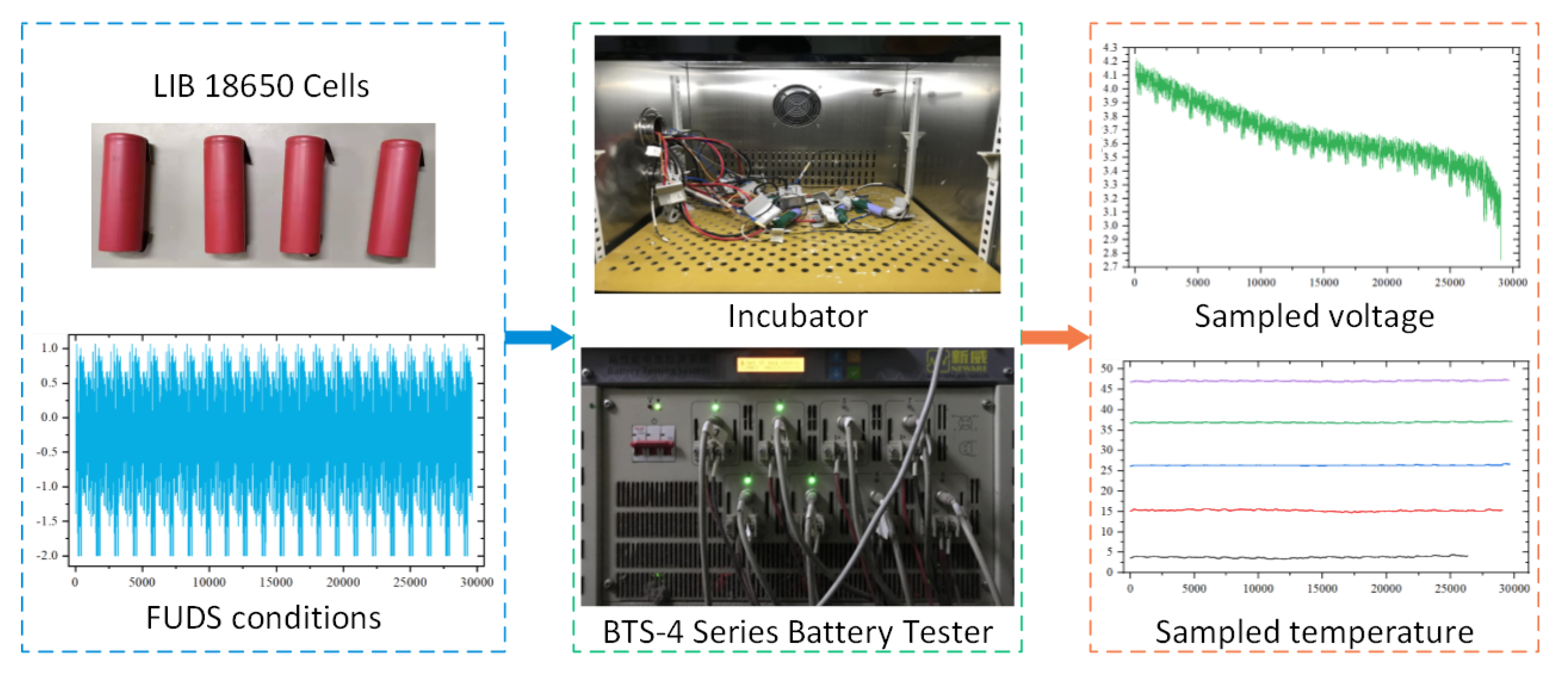
4.1. Experiment Setup

Four 18,650 cells are considered as tested objects and numbered as cell1, cell2, cell3, and cell4, and detail parameters are listed in Table 2. The experiment’s setup is shown in Figure 5. FUDS operation condition is applied to the four 18,650 cells from the BTS-4 series battery tester produced by Neware Company to simulate a realistic working situation, and an incubator is included to maintain the environment temperature of the experiments. LIB cells are fully charged by the constant-current constant-voltage (CC-CV) method before applying FUDS; then, the cells are fully discharged to the cut-off voltage of 2.75 V in Table 2 under cycling FUDS periods (a single period in FUDS shown in Figure 6), and data are collected by the tester and sent to a host computer for further processing.
Considering the available capacity of battery cells in realistic working conditions, temperatures induce significant influences on the discharging/charging ability of battery cells from 0 to 100% SOC range, which may cause different SOC-changing trajectories. Hence, experiments under five temperatures were conducted, and the available capacity of the four cells is measured, as shown in Figure 7. Rreal SOC values are calculated by the ampere-hour integral method with the capacity listed in Figure 7. It can be found in Figure 7 that the influence of temperature T t e m p ( t ) cannot be ignored; thus, as the previous section presented, the proposed fPIRNN determines the inputs as x ( t ) = [ x 1 ( t ) , x 2 ( t ) , x 3 ( t ) ] T = [ u t ( t ) , i ( t ) , T t e m p ( t ) ] T and the output as y ( t ) = S O C ( t ) . Figure 8 provides the selected data for the proposed fPIRNN to divide into training, validation, and testing data. The data in this study are sampled by the BTS-4 battery tester in 1Hz frequency. With preprocessing, the total data used for the proposed algorithm are 109,167 sampled points, each of which includes three input dimensions (current, voltage, and temperature) and one output dimension (SOC). The ratio of training, validation, and testing is set as train:valid:test = 0.75:0.05:0.20. Hence, with SOC calculated by the Ah integral method as output targets, the size of the training dataset is 81,875 points, the validation dataset is 5458 points, and the testing dataset is 21,834 points. From Figure 8, the amount of the selected data is over 100 thousand, which can support big-data learning for fPIRNN. The sequential order can be changed to divide data according to different cells or different temperatures.

4.2. Sensitivity of Fractional Order and Impedance

For the hyperparameter optimization of the designed fPIRNN in Figure 4, the sensitivity of parameters related to the fractional-order knowledge should be determined, mainly including the key parameters of FOGDm method and the parameters of fractional-order PDE constraints. We list the unchanged parameters of fPIRNN in Table 3 and determine sensitive parameters with a certain possible range according to the impedance of FOM in (12) and Figure 1. It should be noted that, after conducting a sensitivity analysis, only one set of parameters was selected for comparisons, and it was applied to all estimation conditions to produce an algorithm with GDm and FOGDm, with or without FO constraints that are stable, and to achieve convergence.
To quantize sensitivity, Pearson correlation coefficients are calculated with sampled groups of the nine parameters in Table 3 and the corresponding output performance of fPIRNN. The mean square error (MSE) is selected as the evaluation function of all performances in this study. Specifically, despite the total MSE (marked as p e r f ), the performance of the training dataset, validation dataset, and testing dataset can be seperately presented as t r p e r f , v p e r f , and t p e r f . The correlation coefficients are list in Table 4. Combining Table 3 and Table 4, fractional order α 1 and momentum weight μ in FOGDm method mainly contribute to training performances. The impedance (mainly d s o c and C bat ) of the FOM of LIBs ((12)) has strong correlations with the validation performance and testing performance, while ohm resistance R 0 has weaker influences due to its small magnitude (e-3 level). Loss weights w data and w PDE have the same coefficients because the two parameters hold the following relationship: w PDE = 1 w data .

4.3. Estimation with Fractional-Order Constraints

With preprocessed data and tuned fPIRNN, we conduct SOC estimations under several conditions. This section provides experimental results only with fractional-order constraints in fPIRNN to illustrate the effectiveness of fractional-order PDE constraints. Figure 9 is the training process and output performance, and four snippets under FUDS conditions act as testing data. The parameter tuning is conducted under the instruction of the sensitivity analysis, and focus on several mainly sensitive parameters. The tuning result is as follows: α 1 = 0.9 , μ = 0.75 , η = 0.18 , α 2 = 0.9 , d s o c = 40 , C bat = 20 , R 0 = 5 × 10 3 , w data = 0.8 , and w PDE = 0.2 . According to the tuning result, all parameters of GDm, FOGDm, and FO constraints are set as the same in the following part for comparison purposes. The loss target of training performances is set as L target = 1 × 10 3 . With the MSE of training losses reaching 1 × 10 3 , the average error of SOC estimation can converge within 3.2 % . In Figure 9a, all training, validation, and testing losses can converge to L target , while the outputs in Figure 9b contain substantial noise. The reason for the output’s noise mainly involves two aspects. Firstly, due to dynamic FUDS conditions, the voltage’s inputs change dynamically in the 1Hz frequency, which may introduce increased learning noise for the proposed fPIRNN. Secondly, a large amount of testing data (totally 21,834 points) are plotted in Figure 9, which means that all outputs and errors over 20 thousand are plotted in one figure, and this produces curves that are very intense. Hence, a fitted process is employed for the outputs in this study by a second-order polynomial fitting for improved filtering and the presentation of estimation results (marked as “fitted output”). The corresponding output error is also calculated and marked as “fitted error”, as shown in Figure 9c. The relationships among the variables in Figure 9 and the following figures can be presented as follows:
e r r o r = o u t p u t t a r g e t , f i t t e d o u t p u t = polyfit ( o u t p u t ) , f i t t e d e r r o r = f i t t e d o u t p u t t a r g e t ,
where o u t p u t is the output SOC values, t a r g e t is the SOC target, and “ polyfit ” means the second-order polynomial fitting function.
The converge method in the backpropagation process of training is chosen with the gradient descent with momentum (GDm) method; thus, an RNN with GDm functions as the benchmark for comparison purposes. In Figure 10, the experiment results of fPIRNN with fractional-order PDE constraints and RNN with GDm are presented and marked as “FO constraints” and “GDm”, respectively. Three main aspects of performance were analyzed, that is, convergence process (Figure 10a), output portraits (Figure 10b,c), and estimation accuracy (Figure 10d–f). Although both “FO constraints” and “GDm” can converge near L target within 200 epochs, the convergence speed and achievable loss of fPIRNN with fractional-order constraints are superior to those of RNN with GDm. Under the disturbance of the switching point between two snippets, which have been preprocessed into a time-series sequence, the proposed algorithm can still output the estimated results stably, and the fitted output can follow the target during the entire SOC range (0–100%), as shown in Figure 10c. With respect to the accuracy, less predicted noise in fPIRNN with fractional-order constraints was achieved when comparing Figure 10d,e. Moreover, it seems that the proposed fPIRNN behaves better in high SOC ranges from Figure 10f.
For further illustration, regression analyses and MSE of output error are also calculated, as shown in Figure 11. Higher regression coefficients in Figure 11a mean improved convergence performances relative to the estimated targets, and lower MSE outputs in Figure 11b mean higher accuracy relative to the estimated targets.

4.4. Estimation with Physics-Informed Recurrent Neural Network

This section provides the final version of fPIRNN proposed in this work, that is, fPIRNN with both FOGDm and fractional-order PDE constraints (marked as “FOGDm and FO loss”). FOGDm is also a proposed method in our work, and PINN only with FOGDm acts as the benchmark for comparisons in this section (marked as “FOGDm”). The convergence process (Figure 12a), output portraits (Figure 12b,c), and estimation accuracy (Figure 12d–f) are provided. With FOGDm and fractional-order constraints, the proposed fPIRNN can converge near L target much quicker (within 100 epochs), while FOGDm introduces some unstable fractional-order gradients during the convergence process due to the discrete calculation in (20). Both “FOGDm” and “FOGDm and FO loss” can bring down the estimated error (within 2.5%), as shown in Figure 12f, and fPIRNN with fractional-order constraints still achieves less estimated noise, as shown in Figure 12e.
A regression analysis and MSE of output are provided in Figure 13. We combine the results of the four NN algorithms together: RNN with GDm (“GDm”), fPIRNN only with fractional-order constraints (“FO constraints”), fPIRNN only with FOGDm (“FOGDm”), fPIRNN with both FOGDm and fractional-order constraints (“FOGDm and FO loss”). From Figure 13, the effectiveness of both FOGDm and fractional-order constraints achieved higher regression coefficients and a lower MSE than that in Figure 11, while fractional-order constraints combined with FOGDm (“FOGDm and FO loss”) do not show significant improvements with respect to the performance of the proposed fPIRNN than that only with FOGDm. Considering the results presented from Figure 10 to Figure 13, some key points can be listed as follows.
  • The proposed fPIRNN with FOGDm and FO constraints can control SOC’s estimation accuracy within 8% when coexisting with learning noise and within 2.5% when filtering the noise (“fitted error”);
  • Both FOGDm and fractional-order constraints hold the physics-informed knowledge of LIBs and can optimize the proposed fPIRNN;
  • The FOGDm method for backpropagation not only introduces improved performances than fractional-order constraints but also introduces more training fluctuations and estimation noise;
  • Besides certain enhancements to fPIRNN, fractional-order constraints can also stabilize the output and reduce the output’s noise;
  • FOGDm and fractional-order constraints hold opposite effects on noise, which can compensate with each other, resulting in the final version of fPIRNN in this work.
  • Combined with the design of embedding physics-informed knowledge, specific conditions at low SOC range and high SOC range can also be embedded to increase the prediction accuracy in these crucial ranges.

5. Conclusions

This paper presents a physics-informed recurrent neural network for SOC estimations of LIBs by introducing fractional-order gradients into backpropagation processes and fractional-order constraints into network loss. The fractional-order gradient is designed for weight updates during the backpropagation of algorithm, and the gradient momentum is further developed and added to construct a fractional-order gradient descent method with momentum, named FOGDm. The fractional-order constraint is deduced from the electrochemical relationship described by battery fractional-order models, resulting in a fractional-order PDE form; then, the fractional-order PDE constraint is encoded into the calculation of training loss. Hence, the backpropagation process is enhanced by the proposed FOGDm method with accurate gradient descent directions, and its convergence is optimized by embedding battery information, which allows the proposed fPIRNN to learn battery inputs faster and to estimate the outputs more precisely. Moreover, the generalization capability of ML algorithm is also improved because the battery mechanism acts as a part of the convergence evaluation of the algorithm. In view of the flexible framework with FOGDm and fractional-order constraints, the proposed fPIRNN can also be applied to other state estimation processes (such as capacity, SOH, and RUL) or safety analysis (such as pre-warning and pack heterogeneity) more than SOC estimations. However, the embedded physics in this study is based on a fractional-order ECM, which mainly reflects the electrical characteristics of LIB. For an improvement in the proposed algorithm, PDEs of electrochemical model or other physics-based models with more intensive battery mechanisms can be employed to deduce unsupervised constraints for the loss function. More inner-state variables and knowledge on their reactions related to battery mechanisms can be considered more than the voltages and currents used in this study, which will be the main topic in our future studies.

Author Contributions

Conceptualization, Y.W. and Y.C.; methodology, Y.W. and Y.C.; software, Y.W.; validation, Y.W.; formal analysis, Y.W.; investigation, Y.W. and X.H.; resources, X.H. and D.G.; data curation, D.G. and M.O.; writing—original draft preparation, Y.W.; writing—review and editing, X.H., L.L. and Y.C.; supervision, M.O.; project administration, X.H. and M.O.; funding acquisition, Y.W., X.H. and M.O. All authors have read and agreed to the published version of the manuscript.

Funding

This research was funded by National Natural Science Foundation of China under Grant No. 62103220 and No. 52177217 and Beijing Natural Science Foundation under Grant No.3212031.

Institutional Review Board Statement

Not applicable.

Informed Consent Statement

Not applicable.

Data Availability Statement

Not applicable.

Conflicts of Interest

The authors declare no conflict of interest.

Abbreviations

The following abbreviations are used in this manuscript:
PINNPhysics-informed neural network;
PIRNNPhysics-informed recurrent neural network;
fPIRNNfractional-order physics-informed recurrent neural network;
FOGDFractional-order gradient descent;
FOGDmFractional-order gradient descent with momentum;
FUDSFederal urban driving schedule;
PDEPartial differential equation;
RNNRecurrent neural network;
NNNeural network;
SOCState of charge;
LIBLithium-ion battery;
FOMFractional-order model;
MSEMean square error;
G-LGrünwald–Letnikov;
MLMachine learning;
CPEConstant phase element;
OCVOpen circuit voltage.

References

  1. Yang, R.; Xiong, R.; Ma, S.; Lin, X. Characterization of external short circuit faults in electric vehicle Li-ion battery packs and prediction using artificial neural networks. Appl. Energy 2020, 260, 114253. [Google Scholar] [CrossRef]
  2. Roman, D.; Saxena, S.; Robu, V.; Pecht, M.; Flynn, D. Machine learning pipeline for battery state-of-health estimation. Nat. Mach. Intell. 2021, 3, 447–456. [Google Scholar] [CrossRef]
  3. Schindler, M.; Sturm, J.; Ludwig, S.; Schmitt, J.; Jossen, A. Evolution of initial cell-to-cell variations during a three-year production cycle. ETransportation 2021, 8, 100102. [Google Scholar] [CrossRef]
  4. Tanim, T.R.; Dufek, E.J.; Walker, L.K.; Ho, C.D.; Hendricks, C.E.; Christophersen, J.P. Advanced diagnostics to evaluate heterogeneity in lithium-ion battery modules. ETransportation 2020, 3, 100045. [Google Scholar] [CrossRef]
  5. Wang, Y.; Tian, J.; Sun, Z.; Wang, L.; Xu, R.; Li, M.; Chen, Z. A comprehensive review of battery modeling and state estimation approaches for advanced battery management systems. Renew. Sustain. Energy Rev. 2020, 131, 110015. [Google Scholar] [CrossRef]
  6. Lu, Y.; Li, K.; Han, X.; Feng, X.; Chu, Z.; Lu, L.; Huang, P.; Zhang, Z.; Zhang, Y.; Yin, F.; et al. A method of cell-to-cell variation evaluation for battery packs in electric vehicles with charging cloud data. ETransportation 2020, 6, 100077. [Google Scholar] [CrossRef]
  7. Zahid, T.; Xu, K.; Li, W.; Li, C.; Li, H. State of charge estimation for electric vehicle power battery using advanced machine learning algorithm under diversified drive cycles. Energy 2018, 162, 871–882. [Google Scholar] [CrossRef]
  8. Su, L.; Wu, M.; Li, Z.; Zhang, J. Cycle life prediction of lithium-ion batteries based on data-driven methods. ETransportation 2021, 10, 100137. [Google Scholar] [CrossRef]
  9. Yang, H.; Wang, P.; An, Y.; Shi, C.; Sun, X.; Wang, K.; Zhang, X.; Wei, T.; Ma, Y. Remaining useful life prediction based on denoising technique and deep neural network for lithium-ion capacitors. ETransportation 2020, 5, 100078. [Google Scholar] [CrossRef]
  10. How, D.N.; Hannan, M.; Lipu, M.H.; Ker, P.J. State of charge estimation for lithium-ion batteries using model-based and data-driven methods: A review. IEEE Access 2019, 7, 136116–136136. [Google Scholar] [CrossRef]
  11. Lipu, M.H.; Hannan, M.; Hussain, A.; Ayob, A.; Saad, M.H.; Karim, T.F.; How, D.N. Data-driven state of charge estimation of lithium-ion batteries: Algorithms, implementation factors, limitations and future trends. J. Clean. Prod. 2020, 277, 124110. [Google Scholar] [CrossRef]
  12. Wang, Y.; Wang, L.; Li, M.; Chen, Z. A review of key issues for control and management in battery and ultra-capacitor hybrid energy storage systems. ETransportation 2020, 4, 100064. [Google Scholar] [CrossRef]
  13. Lai, X.; Yi, W.; Cui, Y.; Qin, C.; Han, X.; Sun, T.; Zhou, L.; Zheng, Y. Capacity estimation of lithium-ion cells by combining model-based and data-driven methods based on a sequential extended Kalman filter. Energy 2021, 216, 119233. [Google Scholar] [CrossRef]
  14. Zheng, Y.; Gao, W.; Han, X.; Ouyang, M.; Lu, L.; Guo, D. An accurate parameters extraction method for a novel on-board battery model considering electrochemical properties. J. Energy Storage 2019, 24, 100745. [Google Scholar] [CrossRef]
  15. Wang, Y.; Chen, Y.; Liao, X. State-of-art survey of fractional order modeling and estimation methods for lithium-ion batteries. Fract. Calc. Appl. Anal. 2019, 22, 1449–1479. [Google Scholar] [CrossRef]
  16. Wang, B.; Liu, Z.; Li, S.E.; Moura, S.J.; Peng, H. State-of-charge estimation for lithium-ion batteries based on a nonlinear fractional model. IEEE Trans. Control Syst. Technol. 2016, 25, 3–11. [Google Scholar] [CrossRef]
  17. Nasser-Eddine, A.; Huard, B.; Gabano, J.D.; Poinot, T. A two steps method for electrochemical impedance modeling using fractional order system in time and frequency domains. Control Eng. Pract. 2019, 86, 96–104. [Google Scholar] [CrossRef]
  18. Wang, X.; Wei, X.; Zhu, J.; Dai, H.; Zheng, Y.; Xu, X.; Chen, Q. A review of modeling, acquisition, and application of lithium-ion battery impedance for onboard battery management. ETransportation 2021, 7, 100093. [Google Scholar] [CrossRef]
  19. Tian, J.; Xiong, R.; Yu, Q. Fractional-order model-based incremental capacity analysis for degradation state recognition of lithium-ion batteries. IEEE Trans. Ind. Electron. 2018, 66, 1576–1584. [Google Scholar] [CrossRef]
  20. Zou, C.; Hu, X.; Dey, S.; Zhang, L.; Tang, X. Nonlinear fractional-order estimator with guaranteed robustness and stability for lithium-ion batteries. IEEE Trans. Ind. Electron. 2017, 65, 5951–5961. [Google Scholar] [CrossRef]
  21. Li, S.; Hu, M.; Li, Y.; Gong, C. Fractional-order modeling and SOC estimation of lithium-ion battery considering capacity loss. Int. J. Energy Res. 2019, 43, 417–429. [Google Scholar] [CrossRef] [Green Version]
  22. Sulzer, V.; Mohtat, P.; Aitio, A.; Lee, S.; Yeh, Y.T.; Steinbacher, F.; Khan, M.U.; Lee, J.W.; Siegel, J.B.; Stefanopoulou, A.G.; et al. The challenge and opportunity of battery lifetime prediction from field data. Joule 2021, 5, 1934–1955. [Google Scholar] [CrossRef]
  23. Feng, X.; Merla, Y.; Weng, C.; Ouyang, M.; He, X.; Liaw, B.Y.; Santhanagopalan, S.; Li, X.; Liu, P.; Lu, L.; et al. A reliable approach of differentiating discrete sampled-data for battery diagnosis. ETransportation 2020, 3, 100051. [Google Scholar] [CrossRef]
  24. Ng, M.F.; Zhao, J.; Yan, Q.; Conduit, G.J.; Seh, Z.W. Predicting the state of charge and health of batteries using data-driven machine learning. Nat. Mach. Intell. 2020, 2, 161–170. [Google Scholar] [CrossRef] [Green Version]
  25. Tian, J.; Xiong, R.; Shen, W.; Lu, J.; Yang, X.G. Deep neural network battery charging curve prediction using 30 points collected in 10 min. Joule 2021, 5, 1521–1534. [Google Scholar] [CrossRef]
  26. Hong, J.; Wang, Z.; Chen, W.; Wang, L.; Lin, P.; Qu, C. Online accurate state of health estimation for battery systems on real-world electric vehicles with variable driving conditions considered. J. Clean. Prod. 2021, 294, 125814. [Google Scholar] [CrossRef]
  27. Chen, Z.; Zhao, H.; Zhang, Y.; Shen, S.; Shen, J.; Liu, Y. State of health estimation for lithium-ion batteries based on temperature prediction and gated recurrent unit neural network. J. Power Sources 2022, 521, 230892. [Google Scholar] [CrossRef]
  28. Han, X.; Feng, X.; Ouyang, M.; Lu, L.; Li, J.; Zheng, Y.; Li, Z. A comparative study of charging voltage curve analysis and state of health estimation of lithium-ion batteries in electric vehicle. Automot. Innov. 2019, 2, 263–275. [Google Scholar] [CrossRef] [Green Version]
  29. Zhu, J.; Wang, Y.; Huang, Y.; Bhushan Gopaluni, R.; Cao, Y.; Heere, M.; Mühlbauer, M.J.; Mereacre, L.; Dai, H.; Liu, X.; et al. Data-driven capacity estimation of commercial lithium-ion batteries from voltage relaxation. Nat. Commun. 2022, 13, 1–10. [Google Scholar] [CrossRef]
  30. Hu, T.; He, Z.; Zhang, X.; Zhong, S. Finite-time stability for fractional-order complex-valued neural networks with time delay. Appl. Math. Comput. 2020, 365, 124715. [Google Scholar] [CrossRef]
  31. Huang, Y.; Yuan, X.; Long, H.; Fan, X.; Cai, T. Multistability of fractional-order recurrent neural networks with discontinuous and nonmonotonic activation functions. IEEE Access 2019, 7, 116430–116437. [Google Scholar] [CrossRef]
  32. Alsaedi, A.; Ahmad, B.; Kirane, M. A survey of useful inequalities in fractional calculus. Fract. Calc. Appl. Anal. 2017, 20, 574–594. [Google Scholar] [CrossRef]
  33. Zhang, Q.; Shang, Y.; Li, Y.; Cui, N.; Duan, B.; Zhang, C. A novel fractional variable-order equivalent circuit model and parameter identification of electric vehicle Li-ion batteries. ISA Trans. 2019, 97, 448–457. [Google Scholar] [CrossRef]
  34. Khan, S.; Ahmad, J.; Naseem, I.; Moinuddin, M. A novel fractional gradient-based learning algorithm for recurrent neural networks. Circuits, Syst. Signal Process. 2018, 37, 593–612. [Google Scholar] [CrossRef]
  35. Chen, Y.; Gao, Q.; Wei, Y.; Wang, Y. Study on fractional order gradient methods. Appl. Math. Comput. 2017, 314, 310–321. [Google Scholar] [CrossRef]
  36. Karniadakis, G.E.; Kevrekidis, I.G.; Lu, L.; Perdikaris, P.; Wang, S.; Yang, L. Physics-informed machine learning. Nat. Rev. Phys. 2021, 3, 422–440. [Google Scholar] [CrossRef]
  37. Han, X.; Ouyang, M.; Lu, L.; Li, J.; Zheng, Y.; Li, Z. A comparative study of commercial lithium ion battery cycle life in electrical vehicle: Aging mechanism identification. J. Power Sources 2014, 251, 38–54. [Google Scholar] [CrossRef]
  38. Guo, D.; Yang, G.; Feng, X.; Han, X.; Lu, L.; Ouyang, M. Physics-based fractional-order model with simplified solid phase diffusion of lithium-ion battery. J. Energy Storage 2020, 30, 101404. [Google Scholar] [CrossRef]
  39. Guo, D.; Yang, G.; Han, X.; Feng, X.; Lu, L.; Ouyang, M. Parameter identification of fractional-order model with transfer learning for aging lithium-ion batteries. Int. J. Energy Res. 2021, 45, 12825–12837. [Google Scholar] [CrossRef]
  40. Tian, J.; Xiong, R.; Lu, J.; Chen, C.; Shen, W. Battery state-of-charge estimation amid dynamic usage with physics-informed deep learning. Energy Storage Mater. 2022, 50, 718–729. [Google Scholar] [CrossRef]
  41. Li, W.; Zhang, J.; Ringbeck, F.; Jöst, D.; Zhang, L.; Wei, Z.; Sauer, D.U. Physics-informed neural networks for electrode-level state estimation in lithium-ion batteries. J. Power Sources 2021, 506, 230034. [Google Scholar] [CrossRef]
Figure 1. Structure of typical FOMs for LIBs: (a) second-order FOM. (b) Simplified FOM.
Batteries 08 00148 g001
Figure 2. Structure of a typical RNN.
Batteries 08 00148 g002
Figure 3. PDE constraints for the ML algorithm to achieve PINN.
Batteries 08 00148 g003
Figure 4. Framework of the proposed PIRNN with fractional-order constraints.
Batteries 08 00148 g004
Figure 5. Experiment setup.
Batteries 08 00148 g005
Figure 6. Current profile of a single period in FUDS.
Batteries 08 00148 g006
Figure 7. The measured capacity of four 18650 cells under five temperatures ( 5 C , 15 C , 25 C , 35 C , and 45 C ).
Batteries 08 00148 g007
Figure 8. Selected data for training, validation, and testing of the algorithm. (a) current profile, containing cycling FUDS periods, (b) measured cell voltage, (c) five measured temperature ( 5 C , 15 C , 25 C , 35 C , 45 C ), and (d) calculated SOC, as output target. Data are collected together in time series (1Hz frequency) and can exchange the sequential order to achieve different division patterns.
Batteries 08 00148 g008
Figure 9. Training process and output performance of fPIRNN. (a) Training, validation, and testing loss; (b) output SOC with fitting; (c) output errors.
Batteries 08 00148 g009
Figure 10. Experiment results of fPIRNN with fractional-order PDE constraints and RNN with GDm. (a) training and testing loss (marked as “training GDm”, “testing GDm”,“training FO constraints”, and “testing FO cosntraints”), (b) estimated SOC with GDm, (c) estimated SOC with FO constraints, (d) estimated error with GDm, (e) estimated error with FO constraints, and (f) comparison of fitted errors.
Batteries 08 00148 g010
Figure 11. Comparison of output performance of fPIRNN with fractional-order constraints to RNN with GDm. (a) Regression coefficient and (b) MSE of output error. “data” means the entire dataset including training, validation, and testing data. Moreover, “training”, “validation”, and “testing” are the corresponding results of the three datasets, respectively.
Batteries 08 00148 g011
Figure 12. Experiment results of fPIRNN with FOGDm and fPIRNN with FOGDm and FO loss. (a) training and testing loss, (b) output SOC with FOGDm, (c) output SOC with FOGDm and FO loss, (d) estimated error with FOGDm, (e) estimated error with FOGDm and FO loss, and (f) comparison of fitted errors.
Batteries 08 00148 g012
Figure 13. Comparison of output performance of four NN algorithms (marked as “GDm”, “FO constraints”, “FOGDm”, and “FOGDm and FO loss”). (a) Regression coefficient and (b) MSE of output.
Batteries 08 00148 g013
Table 1. Training procedure of the PIRNN with fractional-order constraints.
Procedure 3.1 Training details of fPIRNN for SOC estimation of LIBs
input:Sampled dataset D = { ( x 1 , 1 , x 1 , 2 , x 1 , 3 , y 1 ) , ( x 2 , 1 , x 2 , 2 , x 2 , 3 , y 2 ) , , ( x n , 1 , x n , 2 , x n , 3 , y n ) }
step 1Construct a basic RNN with specific hidden layers, neurons, and state feedbacks.
step 2Divide dataset into training dataset, validation dataset, and testing dataset.
step 3Initialization. Specify the initial parameters values of fPIRNN, weight W p 0 , epoch threshold E max , learning rate η , fractional order α , desired loss L target .
step 4While epoch ≤ threshold E p o c h max :
Forward propagation, calculate neuron states by (13) and (14) from input to output.
Calculate the measured loss of the output L data .
Calculate the PDE loss L PDE under the FO constraints by (24), (31), and (32).
Calculate training loss L with L data and L PDE .
Backpropagation, update weights W p with the FOGDm method by (20).
Epoch = epoch +1
step 5If L achieves L target :
training finished;
else:
adjust setup and back to step2 to re-train.
output:Trained fPIRNN with stable parameters, which can make predictions at the testing dataset.
Table 2. LIB 18650 cell parameters.
ParametersValuesParametersValues
rated capacity (0.5 C 5 A)2000 mAhrated voltage3.7 V
max charge voltage4.2 Vdischarge cut-off voltage2.75 V
max charging current1 C 5 Amax discharging current2 C 5 A
working temperature (charge) 0 C 45 C working temperature(discharge) 20 C 60 C
Table 3. Unchanged parameters and sensitive parameters of the proposed fPIRNN.
TypeNameValue/RangeAttribution
Unchanged
parameters
hidden layers1fPIRNN structure
hidden neurons12
max epoch E max 1500
performance functionMSE
train:valid:test0.75:0.05:0.20
Sensitive
parameters
fractional order α 1 [ 0.1 , 1 ] FOGDm in (20)
momentum weight μ [ 0.1 , 1 ] FOGDm in (20)
learning rate η [ 0.08 , 0.26 ] FOGDm in (20)
fractional order α 2 [ 0.1 , 1 ] FO PDE f S O C ( x , t ) in (31)
ratio of OCV-SOC d s o c [ 5 , 50 ] FO PDE f S O C ( x , t ) in (31)
capacitance C bat [ 2.5 , 25 ] FO PDE f S O C ( x , t ) in (31)
ohm resistance R 0 [ 5 × 10 3 , 6 × 10 3 ]FO PDE f S O C ( x , t ) in (31)
loss weight w data [ 0.1 , 1 ] final loss L in (22)
loss weight w PDE 1 w data final loss L in (22)
Table 4. Correlation coefficients of performance with sensitive parameters.
Performance α 1 μ η α 2 d soc C bat R 0 w data w PDE
p e r f 0.2787 0.43080.21400.10050.26850.22240.29020.27750.2775
t r p e r f 0.27940.44200.19900.09640.35660.16040.26220.25040.2504
v p e r f 0.08020.09460.27940.01890.81630.44650.208210.28870.2887
t p e r f 0.02710.10530.10110.03750.76900.55910.24870.22330.2233
Publisher’s Note: MDPI stays neutral with regard to jurisdictional claims in published maps and institutional affiliations.

