Ferromagnetic Resonance in Magnetic Oxide Nanoparticules: A Short Review of Theory and Experiment

Abstract

This review article aims to provide a comprehensive overview of recent FMR studies on magnetic oxide nanoparticles and their potential applications. The use of the FMR technique is a powerful tool to study the magnetic properties of magnetic nanoparticles and can provide valuable information on their behavior. For this, we will start by discussing the purpose of these magnetic nanoparticles and their application in various fields, including biomedical applications, energy storage, and environmental remediation. We will then discuss the methods used to prepare magnetic nanoparticles and the theory behind FMR including the superparamagnetic effect. Additionally, we will present the most recent studies on FMR for magnetic oxide nanoparticles by highlighting the effect of temperature and doping on the magnetic properties of these nanoparticles.

1. Introduction

Magnetic nanoparticles have attracted significant attention in recent years due to their unique magnetic properties and potential applications in various fields, such as biomedicine, energy, and information technologies. Several techniques have been used to investigate the magnetic properties of nanoparticles, including ferromagnetic resonance (FMR) [1]. Indeed, FMR has been extensively studied in bulk magnetic materials, including thin films, and more recently, in magnetic nanoparticles. In these nanoscaled particles, the FMR behavior can be affected by a variety of factors, such as size, shape, surface effects, and composition [2]. Thus, the study of magnetic nanoparticles by FMR can provide in-depth information on the intrinsic and extrinsic magnetic properties of these particle systems.

The application of nanoparticles could revolutionize many sectors of our society. In biomedicine, magnetic nanoparticles are being explored for a range of applications, such as magnetic resonance imaging (MRI), drug delivery, and hyperthermia treatment of cancer [3]. In MRI, magnetic nanoparticles can be used as contrast agents to improve sensitivity. In drug delivery, magnetic nanoparticles can be functionalized with drugs and targeted to specific cells or tissues using an external magnetic field [4]. In hyperthermia treatment, magnetic nanoparticles can be used to selectively heat tumor cells, leading to their destruction [3].

In addition to biomedicine, magnetic nanoparticles are also being investigated for energy storage devices, such as batteries and supercapacitors, due to their high surface area and tunable magnetic properties [5]. Finally, magnetic nanoparticles can be used in information technology, particularly in magnetic data storage and spintronics [6,7]. Indeed, magnetic data storage is a widely used technology in hard drives. Magnetic nanoparticles can be used to develop spin-based electronic devices, which could have lower power consumption, higher speeds, and greater storage densities than traditional electronic devices [8,9].

2. Ferromagnetic Resonance

To study the magnetic properties of magnetic nanoparticles, magnetization dynamics can be a useful tool. Indeed, the magnetization dynamics allow us to understand how the magnetization of such particles responds to external stimulation such as magnetic fields and electromagnetic pulses. Thus, by measuring the magnetic response, one can provide information on the intrinsic properties of the nanoparticles, such as their magnetization, magnetic anisotropy, and magnetic relaxation times. Furthermore, magnetization dynamics is also useful for studying the magnetic interactions between nanoparticles, such as the dipole–dipole interaction and exchange interactions. It is well known that these interactions can have a significant effect on the magnetic properties of nanoparticle assemblies.

Historically, the first studies of magnetization dynamics were performed in the early 20th century. Over the past few decades, techniques for investigating magnetization dynamics have considerably developed. This research particularly concerns nanostructured magnetic materials due to their potential applications in the field of spintronics [10].

Magnetization dynamics can occur over a wide range of time scales. Figure 1 shows different types of magnetization dynamics with their characteristic time scales ($\tau$). These time scales depend on the dimensions of the magnetic system, its parameters, and the type of excitation. Magnetization dynamics are then classified into two main categories depending on their characteristic times: fast, where $\tau$ is on the order of nanoseconds to hundreds of picoseconds, and ultra-fast, with $\tau$ on the order of sub-picoseconds. In magnetic nanoparticles, the magnetization reversal process is classified as fast magnetization dynamics.

In order to study magnetization dynamics, different techniques exist and can be classified into two groups: time-domain methods and frequency-domain methods [10].

Time-domain techniques involve measuring the temporal response of the magnetization following an external excitation, such as an ultra-short laser pulse or a pulsed magnetic field. Frequency-domain techniques are based on the precessional frequency measurement of the resonance field for a fixed frequency-driven resonance as performed in microwave spectroscopy.

The operating principles of FMR techniques are based on the use of a combination of a microwave field ($h_{rf}$) and a static magnetic field. The small $h_{rf}$ field excites the spin system while the static field is slowly swept through a specific field range. At a specific value of the applied field, the precessional amplitude becomes maximum. This corresponds to the resonance field of the specific value at the driving $h_{rf}$ frequency.

Several varieties of FMR exist: by far the most common methods are cavity FMR and broadband FMR, such as VNA-FMR (vector network analyzer FMR). In cavity FMR, the sample is placed in a resonant cavity of a microwave spectrometer and the reflected power is measured. This measurement is extremely sensitive because the quality factor of the cavity is generally very high, which allows for the study, for example, of thin layers of a few nanometers in thickness. VNA-FMR is a highly effective frequency-sweeping technique. The sample is placed on a coplanar waveguide (CPW) which is connected to the VNA. The VNA serves as both a source and detector of the radiofrequency signal and compares the incoming and outgoing signals (their amplitude and phase), allowing for the measurement of sample absorption as a function of frequency and field.

Compared to other techniques for measuring magnetization dynamics, FMR techniques have several advantages; in particular, their high sensitivity. Indeed, FMR can detect very small changes in the magnetic properties of a material, which makes it useful for studying nanostructures. FMR is a non-destructive technique, which means that it does not damage the sample being measured, which allows for repeated measurements on the same sample over time. Moreover, FMR can measure magnetic properties over a wide range of frequencies (VNA-FMR), up to tens of gigahertz and even hundreds, which makes it useful for studying magnetic properties at high frequencies. Finally, FMR is a simple technique to implement, does not require complex equipment, and can be used to study a wide range of magnetic materials, including ferromagnetic, antiferromagnetic, and ferrimagnetic materials, as well as magnetic thin films, nanoparticles, and nanostructured systems.

In conclusion, ferromagnetic resonance is an excellent technique to study and understand the phenomena that govern the magnetic properties of nanoparticles. This investigation will allow us to tune magnetic properties depending on the desired application. Further research in this area is expected to lead to the development of new devices with improved performance.

3. Methods of Synthesis

Synthesizing magnetic nanoparticles with precise control of their size, shape, and magnetic properties is crucial for achieving optimal performance for the desired applications. There are various methods for synthesizing magnetic nanoparticles, which are subdivided into two main categories, “physical” and “chemical” methods [3], including chemical precipitation, co-precipitation, sol-gel, hydrothermal, and laser evaporation methods..., etc. [11].

In this section, we will discuss two typical chemical methods, i.e., the sol-gel and hydrothermal methods, which are widely used for synthesizing magnetic nanoparticles. These methods have unique advantages where understanding their processes is essential for using the potential of magnetic nanoparticles in various applications. We have chosen these two techniques because they are the most used for nanoparticle synthesis in this review.

3.1. Sol-Gel Technique

The sol-gel method is commonly used for synthesizing magnetic nanoparticles. This method involves the preparation of a solution (sol) that is then transformed into a solid or (gel) through a series of chemical reactions [11].

To produce magnetic nanoparticles using the sol-gel method, the first step is to prepare a sol of the desired metal salts. This is achieved by dissolving the metal salts in a solvent, such as water or ethanol [12], and then adding a stabilizing agent, such as a surfactant or polymer, to prevent the particles from agglomerating. To transform the sol into a gel, the obtained solution is then exposed to a series of chemical reactions, including hydrolysis and condensation. The gel is then dried and annealed to remove any remaining solvent. During calcination, the gel is heated to high temperatures, which causes the metal ions to form metal oxide nanoparticles [13]. The metal oxide nanoparticles are typically coated with a magnetic material, such as iron oxide or cobalt. This is performed by using a variety of techniques, such as the addition of a magnetic precursor to the sol before gelation.

An example of this technique of ${\mathrm{MgZnFe}}_2{\mathrm{O}}_4$ nanoparticle synthesis is illustrated in Figure 2. The nanoparticles are prepared by a primary mixture of different solutions. The mixtures are then slowly dissolved in distilled water with stirring, to form a red, dish gel. The gel is then dried at 150 °C by placing it in a furnace. The nanoparticles were then produced by grinding the obtained substance, which is finally annealed at 750 °C for one hour to complete the chemical process.

The resulting magnetic nanoparticles are highly stable with good control of the particle size. The sol-gel method is considered to be a powerful tool for the synthesis of magnetic nanoparticles with precise control over their size, shape, and magnetic properties. However, this technique also has several disadvantages including a long time of reaction and the use of toxic organic solvents [3]. By manipulating the sol composition, reaction conditions, and post-synthesis treatments, it is possible to tailor the properties of the nanoparticles.

3.2. Hydrothermal Technique

Hydrothermal synthesis is a popular method to produce magnetic nanoparticles with a narrow size distribution, high crystallinity, and excellent magnetic properties. The nanoparticle production process involves the reaction of a precursor solution containing metal ions at high temperatures and pressure. These conditions promote the formation of nuclei, which can grow into magnetic nanoparticles.

The ion metal solution is prepared by dissolving metal salts in water or other solvents. The choice of solvent depends on the nature of the metal ions and their solubility. The hydrothermal process is then carried out in an autoclave, a closed vessel known to resist high temperatures and pressures. The precursor solution is added to the autoclave and then sealed before being heated to temperatures typically ranging from 100 °C to 300 °C. The pressure inside the autoclave is maintained by adding an inert gas such as nitrogen. The nanoparticles are formed by the reaction between the metal ions in the precursor solution with hydroxide ions or other chemical species.

The reaction rate, size, and morphology of the nanoparticles depend on several factors, such as the concentration of the precursor solution, temperature, pressure, and reaction time. The reaction usually lasts several hours to ensure the complete conversion of the metal ions into nanoparticles. After that, the autoclave is cooled, typically at room temperature, and the nanoparticles are recovered by centrifugation or other separation techniques before being washed and dried [14]. An example of ${\mathrm{Fe}}_3{\mathrm{O}}_4$ nanoparticle production by the hydrothermal method is shown in Figure 3 [15]. The synthesis of these particles was carried out at up to 180 °C temperatures for 16 h. ${\mathrm{FeCl}}_3$ and ${\mathrm{FeCl}}_2$ were used as precursor salts, and polyethylene glycol (PEG-400) as surfactant.

The hydrothermal process can produce nanoparticles with different magnetic properties by varying the reaction conditions. For example, different crystal phases can be synthesized for iron oxide such as magnetite ${\mathrm{Fe}}_3{\mathrm{O}}_4$ and maghemite $\gamma$-${\mathrm{Fe}}_2{\mathrm{O}}_3$. In summary, hydrothermal synthesis is a versatile method for producing magnetic nanoparticles with tailored properties and good crystallinity but has the disadvantage of needing high temperature and pressure for the nanoparticle synthesis [3].

4. Aspects of Ferromagnetic Resonance in Magnetic Nanoparticle Assemblies

4.1. General Theory of Ferromagnetic Resonance

The discovery of the phenomenon of ferromagnetic resonance absorption dates to the early work of V. K. Arkad’yev [16] with the observation of the selective absorption of centimeter radio waves in Fe and Ni wires. The theory of ferromagnetic resonance is well established and can be dated from the early work of Landau and Lifshitz [17] with the phenomenological expression of the time-varying magnetization vector as a function of the magnetic torque in the vector product of the magnetization with the magnetic field vector. In its most simple form, the precessional motion of the magnetization vector can be expressed, neglecting the effects of relaxation, as:

$$\frac{\partial \mathbf{M}}{\partial t}={\mu }_0\gamma (\mathbf{M}\times {\mathbf{H}}_{eff})$$

(1)

In this equation, the magnetization is represented by a classical vector, $\mathbf{M}$, of constant length. The magnetic field vector, ${\mathbf{H}}_{eff}$, is an effective field representing the contributions from the externally applied magnetic fields (both static and dynamic), $\mathbf{H}\left(t\right)={\mathbf{H}}_0+\mathbf{h}\left(t\right)$, and internal fields created by magnetic anisotropies (shape and magnetocrystalline) as well as exchange fields. Thus, the effective field is represented as a vector sum of these contributions. The thermodynamic equilibrium of the system is governed by this internal field and will determine the equilibrium orientation of the magnetization, such that the magnitude of the effective field can be expressed as a function of the free energy, E, of the spin system:

$${\mu }_0{\mathbf{H}}_{eff}=-\frac{\partial E}{\partial M}$$

(2)

It is thus possible to determine the equilibrium orientation of the magnetization, denoted by the polar and azimuthal angles for this vector ${\theta }_0,{\varphi }_0$, from:

$$\frac{\partial E}{\partial \theta }=0;\frac{\partial E}{\partial \varphi }=0$$

(3)

The solution of these equations will provide the state for which the free energy is a minimum. These can be rather complex and can require computational analysis, with analytical expressions for the resonance frequency only being possible for specific cases, such as when the applied field is aligned along certain anisotropy and principal axes. Again, the assumption of homogeneous magnetization is a requirement for the solution to these conditions. It is also possible to express the resonance condition between the effective magnetic field, the frequency of precession, and the second (partial) derivatives of the free energy with respect to the angles in the form [18]:

$$\omega ={\mu }_o\gamma {\mathbf{H}}_{eff}=\frac{{\mu }_o\gamma }{M_{s}sin{\theta }_0}{\left[\frac{{\partial }^{2}E}{\partial {\theta }^2}\frac{{\partial }^{2}E}{\partial {\varphi }^2}-{\left(\frac{{\partial }^{2}E}{\partial \theta \partial \varphi }\right)}^2\right]}^{\frac{1}{2}}$$

(4)

This expression, also known as the Smit-Beljers equation [19], provides a convenient relation that only requires the appropriate form of the free energy of the system, from which the derivatives can be calculated. Typically, we can express the free energy (which will in principle contain the same contributions as the effective field) as the sum of the individual contributions:

$$E=E_0+E_{dem}+E_{anis}+E_{exch}+...$$

(5)

where $E_0=-{\mu }_0\mathbf{M}·{\mathbf{H}}_{\mathbf{0}}$ is the Zeeman energy; $E_{dem}$ is the demagnetization energy, which depends on the sample shape and hence the magnetostatic energy; $E_{anis}$ is the magnetocrystalline anisotropy energy, which will depend on the crystalline structure of the sample and internal strains; $E_{exch}$ is the exchange energy, which is also structure dependant and is defined by the exchange interaction between neighboring spins. Other contributions to the free energy of the system may be considered and will depend on the nature of the samples under investigation. This approach must therefore adapt the form of the free energy to the system that is being studied.

4.2. Contributions to the Free Energy in Magnetic Nanoparticle Systems

In the specific case of assemblies of ferromagnetic nanoparticles (NPs), we introduce the terms that are appropriate, such as the specific form of the magnetic anisotropies and the interaction terms between the particles of the assembly, which will typically take the form of the dipolar interaction between pairs of nanoparticles and summed over the assembly. In terms of magnetic anisotropies, there can be several possible contributions, such as bulk-like magnetocrystalline anisotropy energies, which are typically uniaxial but can also contain cubic or hexagonal contributions, depending on the structure of the NPs. Furthermore, since nanoparticles in general have an important proportion of their spins located at or near the surface of the particle, surface anisotropies can also be of importance.

From the expression for the free energy, Equation (5), we can consider the various terms that are applicable and under what conditions. The Zeeman energy term can be expressed as:

$$E_0=-{\mu }_0\mathbf{M}·{\mathbf{H}}_{\mathbf{0}}=-{\mu }_{0}M{H}_0[sin{\Theta }_{H}sin\theta cos(\varphi -{\Phi }_H)+cos{\Theta }_{H}cos\theta ]$$

(6)

where ${\Theta }_H$ and ${\Phi }_H$ denote the polar and azimuthal angles of the applied static field. This term is isotropic, meaning that there is no preferential orientation of the magnetic field with respect to the magnetization as such. It is only under the influence of the anisotropic terms that the free energy will assume an orientational preference in terms of the lowest energy state. Magnetocrystalline anisotropies arise primarily from the spin–orbit interaction and depend on the crystalline structure of the ferromagnetic (ferrimagnetic) material, and they generate easy directions of the magnetization, typically along some principal crystalline axes. Uniaxial anisotropies can arise in several structures, such as hcp cobalt, for which the energy term can be expressed as:

$$E_{uni}^K=K_1^u{sin}^2\theta +K_2^u{sin}^4\theta +...$$

(7)

where the $K_n^u$ are the anisotropy constants that define the strength of the anisotropy and can be determined experimentally. In this expression, it is important to define the coordinate system for which the easy axis coincides with one of the principal axes. Cubic anisotropy is more complex and must incorporate the four-fold symmetry related to a cubic crystalline structure. Cubic structures, as found in some ferromagnetic metals, can exhibit different forms of cubic anisotropy, where easy axes can lie along principal cubic axes, [100], face diagonal [110], or even body diagonal axes [111]. The phenomenological form of the anisotropy energy can be readily found for such systems, and reflect the different symmetries associated with the crystalline directions. For example, Ni, with a cubic fcc structure and an easy axis along the [100] type directions, can be modeled with an anisotropy free energy term of the form [20]:

$$E_{cub}^{\left[100\right]}=K_4{sin}^2\theta +\frac{K_4}{8}(7+cos4\varphi ){sin}^4\theta +...$$

(8)

In the case of bcc Fe, the easy axes lie along body diagonals, for which the free energy can be written as:

$$E_{cub}^{\left[111\right]}=\frac{K_4}{3}\left(1-2{sin}^2\theta +\frac{7}{4}{sin}^4\theta +\sqrt{2}{sin}^3\theta cos\theta sin3\varphi \right)$$

(9)

The shape of a magnetic body can influence the orientation of its magnetization. This is noted most readily in needle-like or elongated forms, where the magnetization tends to align along the long axis to reduce the so-called stray field and has its origin in the dipolar interaction between spins. (As an aside, the dipolar interaction between NPs has a similar effect and can produce an anisotropy in an assembly of NPs due to the spatial distribution of particles.) In the simple case of ellipsoids of rotation, simple analytical expressions can be obtained [18,21,22]. In such cases, a simplified expression for the energy contribution can be written in terms of a demagnetizing tensor, $N_{eff}$, and the demagnetizing field [23]:

$$E_{dem}=-{\mu }_0\mathbf{M}·{\mathbf{H}}_{\mathbf{dem}}=\frac{1}{2}{\mu }_0{M}_s^2{N}_{eff}{cos}^2\theta$$

(10)

We note that the demagnetizing field will align along the direction opposed to the magnetization and hence this energy term is positive. In fact, the form of this equation shows that in many, such as elongated particles, this energy contribution acts as an effective uniaxial anisotropy. Skomski et al. [24] have considered the effective demagnetizing factors for aggregates of particles of different shapes and sample shapes. This can be effectively applied to an assembly of magnetic nanoparticles and will be further discussed in terms of the effective medium later in this article.

Additional anisotropy contributions can arise from the reduced crystalline symmetry at the surface of a nanoparticle. Such contributions occur for smaller NPs, where the number of surface spins represents a significant proportion of the spins in a particle, where particle diameters are of the order of a few nm [25]. The form of the anisotropy energy associated with a surface can be deduced in a similar manner to bulk anisotropies, taking into account the spatial distribution of the neighboring magnetic moments at the crystal (NP) surface. One example of the surface anisotropy energy can be expressed as [26,27]:

$$E_{TSA}=-\sum _i{K}_s{({\mathbf{m}}_i·{\widehat{\mathbf{u}}}_i)}^2$$

(11)

In this model, known as the transverse surface anisotropy model, $K_s$ is the surface anisotropy constant, analogous to the bulk anisotropy constants in Equations (7)–(9), ${\mathbf{m}}_i$ is the unit vector of the magnetization vector, which is assumed to be homogeneous, and ${\mathbf{u}}_i$ represents the unit vector aligned along the direction of the easy axis. The summation (over i accounts for the combined energy of all the spins in a nanoparticle. For the case of uniform magnetization, this term can be replaced by an effective uniaxial term. A more realistic approach can be expressed in the Néel model as [28]:

$$E_{NSA}=-\sum _i\sum _{j\ne i}{K}_s{({\mathbf{m}}_i·{\widehat{\mathbf{u}}}_{ij})}^2$$

(12)

where ${\mathbf{u}}_{ij}={\mathbf{r}}_{ij}/r_{ij}$ is an interatomic unit vector between surface atoms, and ${\mathbf{r}}_{ij}$ is the vector between spins i and j.This will naturally account for the change in symmetry when a surface atom is encountered.

While the anisotropy contributions for a single nanoparticle can be well-defined, in terms of both bulk and surface anisotropies and even in terms of the shape anisotropy for a majority of particle shapes, the situation is more complex when we consider the case of an assembly of nanoparticles. In a vast majority of experimental studies, the NPs are randomly dispersed with random orientations of the anisotropy axes. For large numbers of NPs in a sample, we can average over all directions to give a constant effective anisotropy field, which will in fact be isotropic and homogeneous. Thus we would just have a general uniform increase in the effective energy (or field). An effective anisotropy can be introduced, which incorporates both volume and surface effects, where it is assumed that the overall angular dependence is the same [29]:

$$K_{eff}=K_v+\frac{6}{D}{K}_s$$

(13)

with $K_{v,s}$ being the volume and surface contributions to the total anisotropy, and the factor $(6/D)$ arises from the surface-to-volume ratio for the case of a sphere of diameter D. Herzer [30] has considered the case of randomly oriented nanocrystals in an amorphous magnetic matrix. These systems exhibit very soft magnetic properties, see Herzer (In: [31]) and references therein. In the random anisotropy (RA) model, the overall effect of the individual nanocrystal anisotropies is considered in the assembly. The model was initially developed in order to explain the soft magnetic properties exhibited by amorphous FM materials [32] and further developed by Chudnovsky et al. [33]. By considering an assembly of exchange-coupled nanocrystals of diameter D and volume fraction f with uniaxial magneto-crystalline anisotropy K, the effect of random orientation on the anisotropy axes is obtained by averaging over the N nanocrystals within the FM correlation volume, where $N=f{({\lambda }_{\mathrm{ex}}/D)}^3$ and the correlation volume is $V={\lambda }_{\mathrm{ex}}^3$, where $({\lambda }_{\mathrm{ex}}$ is the exchange length, see Figure 4a. Statistical fluctuations within the exchange volume will give rise to an easy direction for the N crystals and the averaged anisotropy energy will be determined by the fluctuation amplitude. As such, the effective anisotropy constant can be expressed as:

$$<K>\simeq \frac{f{K}_{eff}}{\sqrt{N}}=\sqrt{f}{K}_{eff}{\left(\frac{D}{{\lambda }_{\mathrm{ex}}}\right)}^{\frac{3}{2}}$$

(14)

It is, therefore, seen that the averaging out of the local anisotropy depends on the number of particles within the exchange volume and will only be effective for coupled particles, that is where interactions between the particles exist. Figure 4b illustrates how the local anisotropies are averaged out over an assembly of nanocrystals, see Suzuki and Herzer [34]. The fact that there is a dependency between the averaging of the local anisotropy and the exchange interaction, the exchange length must be renormalized by substituting $<K>$ for K, such that ${\lambda }_{\mathrm{ex}}$ is self-consistent with the averaged anisotropy: ${\lambda }_{\mathrm{ex}}=\sqrt{A/<K>}$, where A is the exchange stiffness constant. From this, we can obtain the following relation:

$$<K>\simeq f^{2}K{\left(\frac{D}{{\lambda }_{\mathrm{ex}}^{\left(0\right)}}\right)}^6=f^2{D}^6\frac{K^4}{A^3}$$

(15)

where ${\lambda }_{\mathrm{ex}}^{\left(0\right)}$ is the characteristic ferromagnetic exchange length and represents the minimum length scale over which the magnetic moments of the particles can vary. If the particle size, D, is less than this value, the magnetization will not follow the randomly oriented easy axis and will be forced to align by the exchange interaction. The arguments used in obtaining this result are valid not only for uniaxial anisotropies and cubic but other symmetries will also apply.

The above discussion refers to the energy contributions of an assembly of non-interacting nanoparticles. In a typical measurement, we generally consider the dynamic response of an assembly of magnetic nanoparticles. In the following, we will show two approaches to this problem. In the first instance, we consider the dipolar interactions between pairs of NPs and then consider how to sum up the contributions of pairs over the entire population of NPs. We start by considering the energy expression for the dipolar interaction between two magnetic NPs, as characterized by their magnetic moments ${\mathbf{m}}_i$ and $\mathbf{m}j$, which we can write as [35]:

$${\epsilon }_{ij}=\frac{{\mu }_0}{4\pi r_{ij}^3}\left[{\mathbf{m}}_i·{\mathbf{m}}_j-3\frac{({\mathbf{m}}_i·{\mathbf{r}}_{ij})({\mathbf{m}}_j·{\mathbf{r}}_{ij})}{r_{ij}^2}\right]$$

(16)

and can be written in terms of the orientation (polar ${\mathsf{\Theta }}_{ij}$ and azimuthal ${\mathsf{\Phi }}_{ij}$ angles) of the vector ${\mathbf{r}}_{ij}$ between the particles, such that:

$${\epsilon }_{ij}=\frac{{\mu }_0{m}_i{m}_j}{4\pi r_{ij}^3}\left\{1-3{[sin{\mathsf{\Theta }}_{ij}cos({\mathsf{\Phi }}_{ij}-\varphi )sin\theta -cos{\mathsf{\Theta }}_{ij}cos\theta ]}^2\right\}$$

(17)

where we consider that the magnetic moments of the particles are aligned parallel with one another. This assumption can be considered to be valid for magnetic NPs with small anisotropies and aligned under the influence of a small magnetic field, such as they would experience during a ferromagnetic resonance experiment. It is interesting to note that this interaction is intrinsically anisotropic, having a minimum energy when the magnetic moments are aligned along the axis separating the particles and a maximum when they are perpendicular to it [36,37]. Since Equation (17) is only the dipolar energy term between two magnetic moments (NPs), we need to make the summations over all N particles in the assembly. Firstly, we can sum the interaction of say a particle i with all the other $(N-1)$ NPs in the assembly. The total dipolar energy for the assembly will then be obtained from the summation of the dipolar energies of all N particles:

$${ϵ}_{Tot}^{DDI}=\frac{1}{2}\sum _i\sum _{j\ne i}{\epsilon }_{ij}$$

(18)

the factor 1/2 is necessary to avoid counting the interactions twice. Let us now consider the summation terms.

$${\epsilon }_{Tot}^{DDI}=\frac{1}{2}\sum _i\sum _{j\ne i}\frac{{\mu }_0{m}_i{m}_j}{4\pi r_{ij}^3}\left\{1-3{[sin{\mathsf{\Theta }}_{ij}cos({\mathsf{\Phi }}_{ij}-\varphi )sin\theta -cos{\mathsf{\Theta }}_{ij}cos\theta ]}^2\right\}$$

(19)

Using the definition of the magnetization as $M=m_i/V_i$, where $V_i$ denotes the volume of the particle labeled i, and that the sum over all particles leads to $V_m={\sum }_i{V}_i$, the magnetic volume of the particle assembly, we can simplify the above expression for a monodisperse assembly (i.e., where all nanoparticles are considered to have the same size and shape, which for simplicity can be considered as spherical). The above expression can now be written as:

$${\epsilon }_{Tot}^{DDI}=\frac{{\mu }_0{M}_s^2{V}_m^2}{8\pi }\sum _i\sum _{j\ne i}\frac{1}{r_{ij}^3}\left\{1-3{[sin{\mathsf{\Theta }}_{ij}cos({\mathsf{\Phi }}_{ij}-\varphi )sin\theta -cos{\mathsf{\Theta }}_{ij}cos\theta ]}^2\right\}$$

(20)

Writing $V_{ij}=4\pi r_{ij}^3/3$, which is the volume of a sphere whose radius is the distance between pairs ($ij$) of particles in the assembly and expressing the term in brackets as $F({\mathsf{\Theta }}_{ij},{\mathsf{\Phi }}_{ij},\theta ,\varphi )$ can now express the dipolar energy as:

$${\epsilon }_{Tot}^{DDI}=\frac{{\mu }_0{M}_s^2{V}_m^2}{6}\sum _{i,j\ne i}\frac{F({\mathsf{\Theta }}_{ij},{\mathsf{\Phi }}_{ij},\theta ,\varphi )}{V_{ij}}$$

(21)

Taking the energy density, $E=\epsilon /V_m$ and expressing the summation as a geometric factor $G({\mathsf{\Theta }}_{ij},{\mathsf{\Phi }}_{ij},\theta ,\varphi )$, the energy density for the dipolar interactions will take the form:

$$E_{Tot}^{DDI}=\frac{{\mu }_0{M}_s^2\nu }{6}G({\mathsf{\Theta }}_{ij},{\mathsf{\Phi }}_{ij},\theta ,\varphi )$$

(22)

where $\nu =V_m/V_s$ is the packing fraction of particles in the sample, where we assume that the sum of the spheres $V_{ij}$ must be proportional to the sample volume, $V_s$, and we further note that any constant of proportionality will be contained within the factor G. The above expression is a convenient form of the dipolar contribution to the total energy and can be considered to contain all the necessary components for nanoparticle assembly. Clearly, the specifics of the spatial distribution must be known for the factor to be evaluated. Indeed, the factor G can be considered as a sample shape function and can be seen to be related to the expression, given below, in the Netzelmann formulation for granular systems. Thus, we can illustrate that the particle volume fraction, $\nu$, and the shape function, G, will determine the overall dipolar energy for a nanoparticle assembly.

To illustrate the significance of the above expression for the dipolar energy, we can consider the case of a spherical spatial distribution of NPs. In effect, the factor G should reduce to unity for the quasi-homogeneous distribution of monodisperse spherical nanoparticles. In this case, Equation (22) reduces to:

$$E_{Tot}^{DDI}=\frac{{\mu }_0{M}_s^2}{6}\nu$$

(23)

Indeed, this expression can be obtained from the demagnetization factor $N_D=1/3$ for a sphere, where the energy contribution is written as $E={\mu }_0{M}_s^2{N}_D/2$. In the above expression, we have the factor $\nu$, which is necessary to account for the reduced magnetic energy for a sample with inferior magnetic content, evenly distributed throughout the sample. We note that this expression is isotropic and has no angular dependence. For non-spherically symmetric samples (NP distributions), the function $G({\mathsf{\Theta }}_{ij},{\mathsf{\Phi }}_{ij},\theta ,\varphi )$, has an angular dependence and reflects the overall shape of the sample and the orientation of the magnetization with respect to the symmetry axes of the spatial distribution shape. We therefore see that the interaction term can be seen to play an identical role as the demagnetizing factor for a magnetic sample. This approach has been applied to the case of discontinuous magnetic multilayers, in which a planar geometry illustrates the importance of this shape distribution effect [38].

Another approach to the problem of nanoparticle arrays can be derived from the consideration of granular systems by Netzelmann [39] and later corrected by Dubowik [40], see also Kakazei et al. [41]. Here, the free energy is expressed in terms of the fraction f of the magnetic particles, which occupy the sample and is given in the form:

$$E_{\nu }=\frac{{\mu }_0}{2}\nu (1-\nu )\mathbf{M}·{\tilde{\mathbf{N}}}_p·\mathbf{M}+\frac{{\mu }_0}{2}{\nu }^2\mathbf{M}·{\tilde{\mathbf{N}}}_s·\mathbf{M}$$

(24)

In this expression, we have ${\tilde{\mathbf{N}}}_{p,s}$, which are the particle (p) and sample (s) shape tensors, and $\nu =V_m/V$ is defined as the ratio of the magnetic to sample volume, respectively. Indeed, this approach is similar to the consideration of the demagnetizing factors for sample and particle as determined by Skomski et al. [24]. We further note that in the case of polydispersion of the nanoparticles, the magnetic volume can be expressed as $V_m=N<V>$, for which the average volume can be obtained from:

$$<V>=\frac{\int VP\left(V\right)\mathrm{d}V}{\int P\left(V\right)\mathrm{d}V}$$

(25)

In this expression, the particle volume distribution is generally given by the log-normal, as given by:

$$P\left(V\right)=\frac{1}{\sqrt{2\pi \sigma V}}{e}^{-{[ln(V/V_0)]}^2/2{\sigma }^2}$$

(26)

where $\sigma$ is the standard deviation of $lnV$ and $V_0$ is the mean value of the particle volume. Given the definitions for $\nu$ and $<V>$, we can further write, $\nu ={\rho }_N<V>$, where ${\rho }_N$ represents the NP density. We note that for the case of spherical particles, the shape factor will be 1/3. Elongated particles can be treated using the Osborn shape factors, such as ellipsoids of rotation. The question of assemblies with randomly oriented NPs can be treated together with the random orientation of the magnetocrystalline anisotropy axes, etc., as considered above.

4.3. Ferromagnetic Resonance in Magnetic Nanoparticle Assemblies

It is possible to combine the two approaches in which we replace the second term in Equation (24) with the dipolar energy, which in fact is another way of looking at the sample shape energy, over the entire NP assembly. We now consider the form of the resonance equation, which can be expressed in the form [36,37]:

$$\frac{sin\theta cos(\theta -{\theta }_0)}{sin{\theta }_0}{H}_r^2+2C\frac{sin\theta cos2{\theta }_0}{sin{\theta }_0}{H}_r-{\left(\frac{\omega }{{\mu }_0\gamma }\right)}^2=0$$

(27)

where the equilibrium polar angle ${\theta }_0$ is defined from the equilibrium condition, as expressed by:

$$Csin2{\theta }_0=H_{r}sin(\theta -{\theta }_0)$$

(28)

In these expressions, the constant C contains various terms depending on the specifics of the magnetic anisotropies relevant to the particles and the assembly. This constant can be expressed in the simplest case for spherical particles as:

$$C=\frac{\pi }{6}MV<r{>}^3$$

(29)

where <r> is the average radius of the NPs. Clearly, this term will be more complex for other forms of particle assembly. For example, Schmool et al. [38] performed calculations for discontinuous multilayer systems.

In the study of Schmool and Schmalzl [36], samples of assemblies of $\gamma$-Fe${}_2$O${}_3$ nanoparticles, with mean particle diameters of 2.7, 4.6, and 7.3 nm, were measured by FMR as a function of the direction of the applied magnetic field, from the perpendicular (0${}^{\circ }$) to the parallel (90${}^{\circ }$) orientations for the NPs distributed in a thin rectangular slab. In Figure 5, we show the angular dependence of the FMR resonance field of NPs with a mean diameter of 4.6 nm. Also shown is the theoretical variation of the resonance field as predicted by Equation (27) and has only an angular dependence due to the dipolar interactions, where we assume the particles are spherical. The points refer to experimental data and the line is the theoretical fit. This curve is representative of all samples measured with other sizes. We observe good agreement between the theory and experimental measurements. This implies that the main influence on the angular-dependent magnetic properties is due to the interparticle interactions and essentially arises from the anisotropy related to the spatial distribution, which in this case was of a thin rectangular slab.

4.4. Superparamagnetism and Its Effect on the Ferromagnetic Resonance of Magnetic Nanoparticles

An important phenomenon in the consideration of the magnetic properties of magnetic nanoparticles and their assemblies is the so-called superparamagnetism to which they are subject. Superparamagnetic effects arise from the thermal fluctuations of the spontaneous magnetization of the nanoparticles and are intimately related to the strength of the magnetic anisotropy of the particles. As the temperature of a sample increases, the thermal energy, denoted as $k_{B}T$, becomes sufficiently large to be able to overcome the energy barrier, which confines the magnetization to a stable configuration (or direction) with respect to the anisotropy axis of the NP, which also depends on the size of the particle itself. These thermal excitations can induce rapid fluctuations of the magnetic moment of the magnetic NP, which in the simplest cases can be described by the Arrhenius law, as expressed by [42]:

$$\tau ={\tau }_0{e}^{E_b/k_{B}T}$$

(30)

where $\tau$ is the superparamagnetic relaxation time and ${\tau }_0$ is a characteristic relaxation time, which, according to the model of Néel-Brown [43,44], is of the order of 10${}^{-13}$–10${}^{-9}$ s. The value of ${\tau }_0$ is often taken to be a constant but actually depends on a number of factors and is weakly temperature dependent. The energy barrier can be represented for the case of a simple uniaxial anisotropy as $E_b=K_{eff}V$, in which $K_{eff}$ is effective anisotropy of the nanoparticle and V its volume. The assumption of Equation (30) is that the nanoparticles are non-interacting. It is worth noting that an applied magnetic field will have the effect of stabilizing the particles, and the relaxation time will be thus modified. This was calculated by Chantrell and Wohlfarth [45], who found a modified relaxation time of:

$$\tau ={\tau }_0{e}^{E_b{(1-H/H_K)}^{\beta }/k_{B}T}$$

(31)

where $H_K=2K/{\mu }_0{M}_s$ is the uniaxial anisotropy field and H the applied field strength. This result derives from the Stoner–Wohlfarth model [46], where an exponent of $\beta =2$ is valid for the applied field along or perpendicular to the uniaxial anisotropy axis [47].

The relationship between the relaxation time, $\tau$, and the characteristic measurement time, ${\tau }_m$, defines two regimes for the behavior of the assembly: i. blocked states and ii. superparamagnetic states, which occur at temperatures below and above the blocking temperature, $T_B$, for which $\tau ={\tau }_m$. In this simple case, DC measurements [48] for the ratio of $ln({\tau }_m/{\tau }_0)$ give a value close to 25, such that:

$$K_{eff}=\frac{k_B{T}_B}{V}ln\left(\frac{{\tau }_m}{{\tau }_0}\right)\simeq 25\frac{k_B{T}_B}{V}$$

(32)

In Figure 6, the effect of size distribution is illustrated, where a distribution of blocking temperatures is predicted for ferromagnetic resonance and SQUID magnetometry [49]. It will be noted that this distribution arises from the volume distribution given in Equation (26) and that $T_B=T_{max}$. Above the blocking temperature, the rapid fluctuations produced by thermal excitations mean that the particles’ magnetic moment reverses between local minima so rapidly that its behavior mimics atomic paramagnetism, and the particle is said to be in the superparamagnetic (SPM) state.

The interactions between magnetic nanoparticles (DDI) can strongly influence the magnetic and superparamagnetic behavior of the NP assembly. The model of Vogel–Fulcher [50] takes into account the interactions and the effect can be observed on the relaxation time of the particles, as shown in the modified formula:

$$\tau ={\tau }_0{e}^{E_b/k_B(T_B-T_0)}$$

(33)

where $T_i$ is an effective temperature, which is proportional to $H_i^2$, with $H_i$ being the the effective interaction field. The Vogel–Fulcher law, as expressed in Equation (33), is only valid for weak interactions. Another form of the modification of the relaxation time due to the effect of interparticle interactions shows the divergence of $\tau$ as the sample is cooled towards the phase transition temperature, such as in the case of spin glasses [51,52]. Here, the relaxation time takes the form:

$$\tau ={\tau }^{\ast }{\left(\frac{T-T_0}{T_0}\right)}^{-z}$$

(34)

where ${\tau }^{\ast }$ is the relaxation time for non-interacting particles and the critical exponent z is of the order of 10.

The interaction via the dipolar forces can often lead to the formation of particle chains [53,54] such as when magnetic nanoparticles are suspended in a fluid. In such cases, the ferromagnetic ordering of the magnetic moments in zero applied fields is favored along the chain direction [42]. Using a mean field model for an infinite chain of magnetic NPs, with separation d, it can be shown that the ordering temperature can be expressed as [42]:

$$T_0=1.202\frac{{\mu }_0}{\pi d^3}\frac{m^2}{3k_B}$$

(35)

where m is the magnetic moment of the particles. The existence of strong dipolar interactions leads to the suppression of superparamagnetic relaxation. A more detailed model for weak fields, as developed by Morup and Tronc [55], can be shown to shift the blocking temperature as a function of the dipolar field, $H_i$, according to the approximate expression:

$$T_B\simeq \frac{KV}{k_{B}ln({\tau }_m/{\tau }_0)}\left\{1-\frac{{\mu }_0{m}^2<H_i>}{{\left(2KV\right)}^2}\left[\frac{4}{3}ln\left(\frac{{\tau }_m}{{\tau }_0}\right)-1\right]\right\}$$

(36)

The strength of the dipolar coupling field can be adjusted by controlling the average separation between the magnetic nanoparticles via preparation techniques, such as coating the NPs with non-magnetic layers. Pereira et al. [56] have shown that this method is effective in adjusting the blocking temperature, where for $\gamma$-Fe${}_2$O${}_3$ nanoparticles with SiO${}_2$ coatings such that:

$$T_B=\frac{1}{ln({\tau }_m/{\tau }_0)}\left(\frac{K_{eff}V+E_{DDI}}{k_B}\right)$$

(37)

This was used to evaluate the effective interaction energy of ∼0.057 eV, for SiO${}_2$ uncoated particles, while for coatings of just under 120 nm, this interaction energy was calculated as ∼0.018 eV.

Temperature-dependent measurements of the FMR have been used to illustrate that the magnetization of the NP assembly conforms to a weighted Langevin function of the form [36]

$$M=M_s\int L\left(\frac{HMV}{k_{B}T}\right)P\left(V\right)\mathrm{d}V$$

(38)

where the particle size distribution is taken into account, Equation (26). The form of the Langevin function can be expressed as $L\left(x\right)=coth\left(x\right)-1/x$. A comparison of the Langevin function with experimental results is illustrated in Figure 7 for $\gamma$-Fe${}_2$O${}_3$ with a mean diameter of 4.6 nm.

The ferromagnetic resonance of assemblies of magnetic NPs has been considered by a number of authors, where the effects of superparamagnetism (SPM) are taken into account [57,58]. In the simple case where spherical nanoparticles, are aligned by the applied field (taken at resonance) in the blocked regime, the resonance equation can be expressed in the form:

$$\frac{\omega }{{\mu }_0\gamma }=H+H_K\left(\psi \right)$$

(39)

where the anisotropy field is expressed as:

$$H_K\left(\psi \right)=\frac{K}{M}(3{cos}^2\psi -1)$$

(40)

where the angle $\psi$ is defined as the angle between the anisotropy axis and the orientation of the magnetization. In the superparamagnetic regime, it is necessary to take into account the thermal fluctuations of the magnetic moments, which gives rise to a dynamic narrowing of the resonance peak and the anisotropy field can be expressed from:

$$H_K\to H_K^{SPM}=H_K\left(\psi \right)<P_2(cos\theta )>=H_K\left(\psi \right)\left(\frac{1-3L\left(x\right)/x}{L\left(x\right)}\right)$$

(41)

where $<P_2(cos\theta )>$ is the second-order Legendre polynomial, $P_2\left(\beta \right)=(3{\beta }^2-1)/2$ and $L\left(x\right)$ is the Langevin function, with $x=MVH/k_{B}T=mH/k_{B}T$. A more realistic model of the SPM regime should also take into account the effect of the size distribution of the NPs in the assembly, as expressed in Equation (38) [59].

4.5. FMR Linewidth

The relation between the resonance linewidth and relaxation processes in magnetic systems means that dynamic studies provide an extremely sensitive probe for such studies. In its most general form, the dynamic response of a magnetic system can be expressed by the Landau–Lifshitz–Gilbert (LLG) equation, which we can write as:

$$\frac{\partial \mathbf{M}}{\partial t}=-\gamma {\mu }_0(\mathbf{M}\times {\mathbf{H}}_{eff})+\frac{\alpha }{M_s}\left(\mathbf{M}\times \frac{\partial \mathbf{M}}{\partial t}\right)$$

(42)

The second term describes the phenomenological damping, which is determined by the size of the Gilbert damping parameter $\alpha$. The linewidth of the resonance from purely Gilbert damping takes the form [60]:

$$\mathsf{\Delta }{H}_G=\frac{4\pi \alpha }{{\mu }_0\gamma }f$$

(43)

showing that the Gilbert damping term is proportional to the frequency of resonance, f. We will not discuss the explicit causes of the linewidth here, see [60] for more details.

The resonance linewidth in magnetic nanoparticle assemblies can be significantly larger than in bulk crystals of the same materials. This extrinsic broadening has a number of mechanisms, and can be generally understood in terms of the magnetic and material inhomogeneities, as expressed by the expression:

$$\mathsf{\Delta }{H}_{NP}=\mathsf{\Delta }{H}_0+\left(\frac{\partial H}{\partial \varphi }\right)\mathsf{\Delta }\varphi +\left(\frac{\partial H}{\partial H_i}\right)\mathsf{\Delta }{H}_i+\left(\frac{\partial H}{\partial V}\right)\mathsf{\Delta }V+\left(\frac{\partial H}{\partial S}\right)\mathsf{\Delta }S$$

(44)

The first term represents the intrinsic linewidth, which can be written as (Vonsovskii, 1966):

$$\mathsf{\Delta }{H}_0=\frac{\alpha }{M_s}\left(\frac{{\partial }^{2}E}{\partial {\theta }^2}+\frac{1}{{sin}^2\theta }\frac{{\partial }^{2}E}{\partial {\varphi }^2}\right)$$

(45)

This expression arises from the fact that the inhomogeneous linewidth broadening must be an explicit function of the orientation of the particle, their volume, and hence, surface area, and this expression is an extension of the arguments of Vittoria et al. [61]. In this way, the angular dependence of the resonance linewidth can be explained as arising from the angular-dependent contributions to the free-energy density. The second term in Equation (44) arises from a spread in crystalline axes, $\varphi$ (not to be confused with the azimuthal orientation of the magnetization). The third term is due to magnetic inhomogeneities in the sample, the fourth term results from the volume distribution of the magnetic particles (a monodisperse system clearly does not contribute since $\mathsf{\Delta }V=0$), and the last term is due to the differences in resonance condition due to surface spins and is proportional to the surface area of the particle S. Bulk systems have negligible contributions because the number of surface spins is appreciable for large magnetic bodies. Equation (44) shows that there will be an explicit dependence of the linewidth on the direction of the applied field, where linewidth broadening will be expected in anisotropic systems. It is noted that assemblies of nanoparticles with broad log-normal distributions can be expected to have very broad resonances; this is indeed the case where measured linewidth can be as large as several kOe.

5. A Compilation of Experimental Studies on FMR

In this section, we will review some recent experimental studies of ferromagnetic resonance and its applications to nanoparticles. Particular attention is given to effects such as temperature (and annealing), doping, and the effects of nanoparticle synthesis techniques and their oxidation.

5.1. Effect of Temperature

The effect of temperature is a critical factor in the understanding of the magnetic properties of ferromagnetic nanoparticles. Indeed, the thermal energy of the system can influence the magnetic moments of the particles, leading to changes in the magnetic properties. In addition, annealing, which is commonly used in the preparation of nanoparticles, can alter the magnetic behavior of the material. Therefore, it is essential to investigate the effects of temperature and annealing on the magnetic properties of ferromagnetic nanoparticles to fully understand their magnetic behavior.

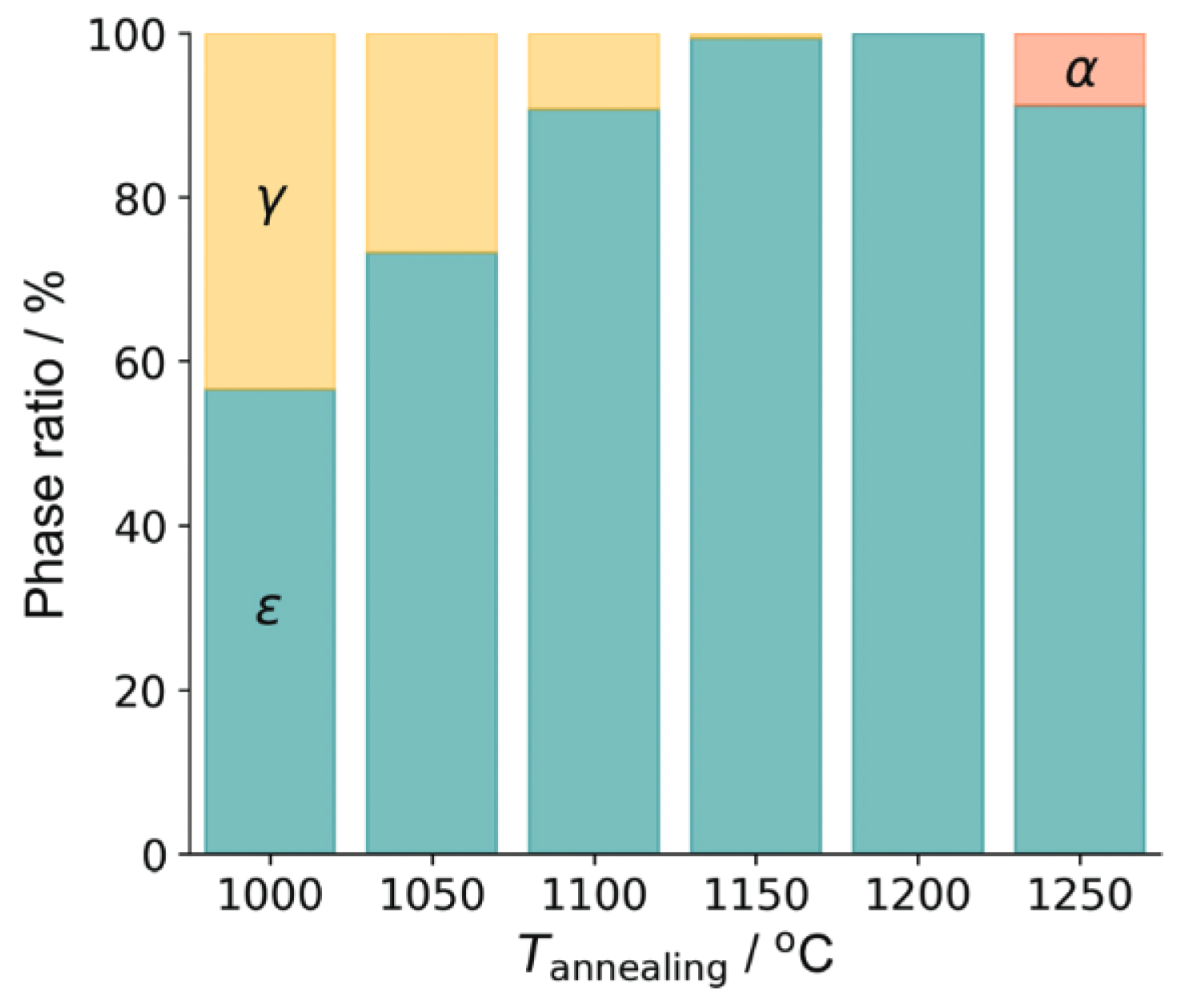
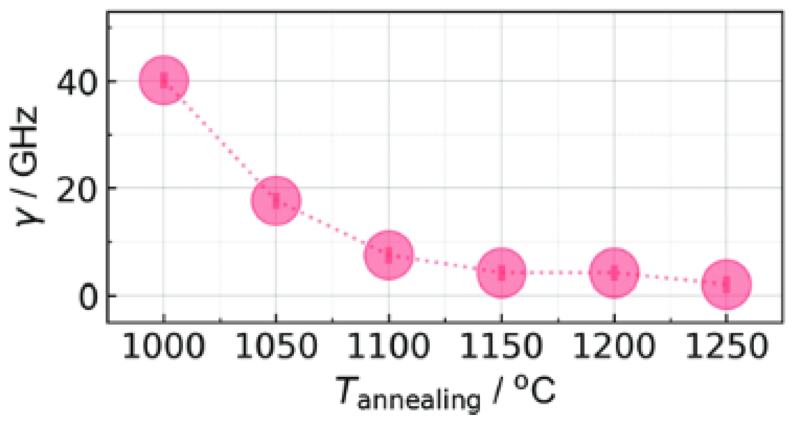
An illustration of these property changes through annealing is shown in Figure 8. The observed increase in the annealing temperature from 1000 °C to 1250 °C allows the formation of different phases ($\gamma$, $ϵ$ and $\alpha$) for ${\mathrm{Fe}}_2{\mathrm{O}}_3$ nanoparticles [62]. In particular, at 1200 °C only the $ϵ-{\mathrm{Fe}}_2{\mathrm{O}}_3$ particle phase is detected. All samples showed a natural ferromagnetic resonance measured by terahertz spectroscopy. This increases from 161 GHz to 170 GHz as the size of iron oxide nanoparticles increases (from 7 to 38 nm) due to annealing, while the half width at half maximum (FWHM represented by factor $\gamma$ in Figure 9) decreases monotonically.

To understand and explain the origin of this variation, it is important to remember that the characteristics of the FMR line are affected by many factors, such as the saturation magnetization, the magnetocrystalline anisotropy, the particles morphology, the thermal fluctuation of magnetization, the demagnetizing field, the porosity of the material, etc.

For these samples, the influence of impurities ($\gamma$ and $\alpha$${\mathrm{Fe}}_2{\mathrm{O}}_3$) can be neglected since their anisotropy fields are much lower than that of the $ϵ$$-{\mathrm{Fe}}_2{\mathrm{O}}_3$[63] and the low spontaneous magnetization leads to very weak demagnetizing fields (less than 100 Oe). Furthermore, the presence of the impurities should not affect the FMR line in the aspect of the porosity of the material as the self-demagnetizing field of the $ϵ$$-{\mathrm{Fe}}_2{\mathrm{O}}_3$ particles is weak (0.9 kOe) with respect to its high anisotropy field (≈40 kOe). Thus, the observed dependence of $\gamma$ (FWHM) on the annealing temperature should be attributed to the variation of the magnetocrystalline anisotropy constant and size of the $ϵ$$-{\mathrm{Fe}}_2{\mathrm{O}}_3$ particles.

Nickel ferrite magnetic nanoparticles annealed at 600 °C, 900 °C, and 1100 °C were studied by FMR in order to investigate the magnetic anisotropy [64]. The samples were prepared by the sol-gel technique and then isothermally treated at different temperatures for 8 h.

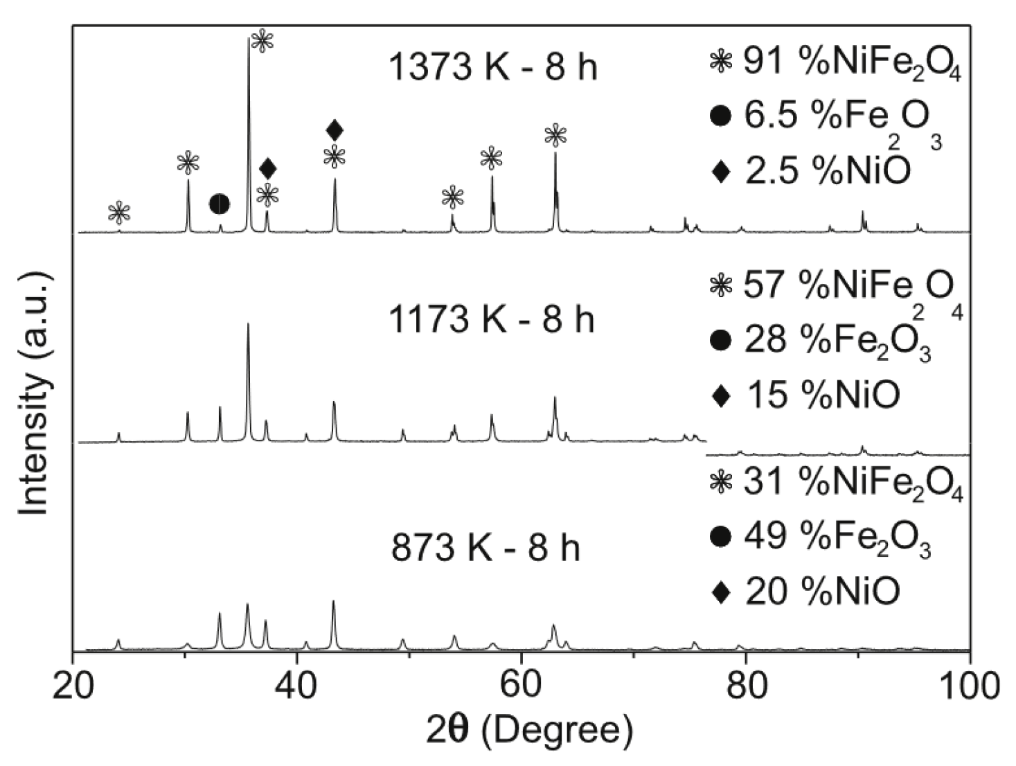
As shown in Figure 10, XRD patterns confirm that the crystalline structure of Ni ferrite particles increases proportionally with the annealing temperature. The nanostructured Ni ferrite particles are ${\mathrm{NiFe}}_2{\mathrm{O}}_4$-based structures and contain different chemical phases such as NiO and ${\mathrm{Fe}}_2{\mathrm{O}}_3$.

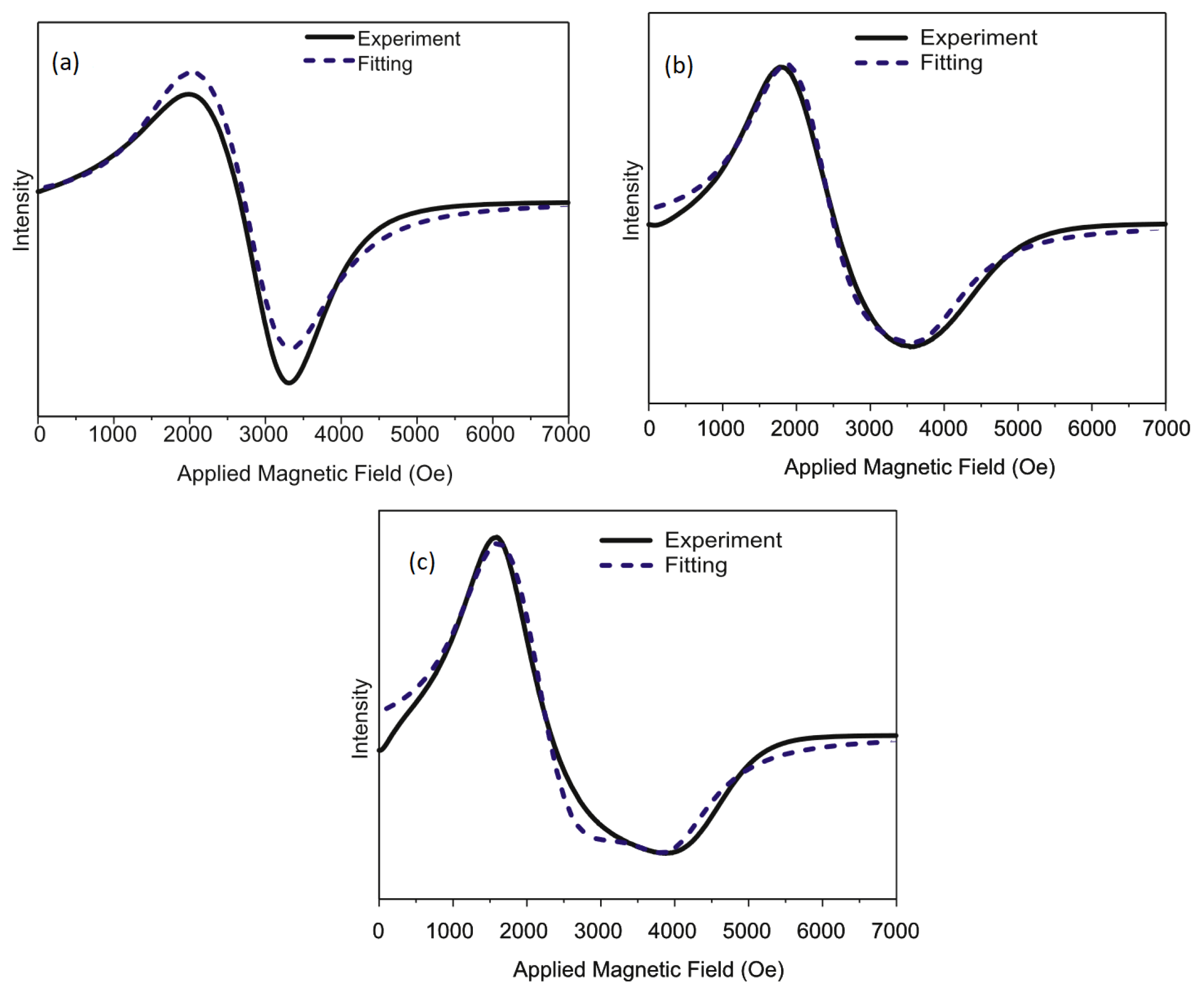
Figure 11 displays the FMR spectra of the three Ni ferrite annealed samples with their theoretical fittings. The model applied to analyze the FMR line was presented by Pessoa et al. in [64,65].

The FMR line fitting results are summarized in

Table 1. FMR data for Ni ferrites. $\mathsf{\Delta }H$ is the linewidth of the FMR absorption line and $H_k$ is the magnetic anisotropy field. Reprinted with permission from M.S. Pessoa, J.R.C. Proveti, F. Pelegrini and P.S. Moscon, Ferromagnetic resonance lines of annealed Ni ferrites, Physica B: Condensed Matter, 558, 20–23. Copyright (2019) Elsevier.

Sample	G-Factor	$\mathbf{\Delta }\mathit{H}$ (Oe)	${\mathit{H}}_{\mathit{k}}$ (Oe)
600 °C	2.6	1640	680
900 °C	2.6	1500	−1200
1100 °C	2.7	900	−1400

. They confirm the presence of the large four-fold cubic magnetic anisotropy as revealed by the XRD data. The FMR line also reveals easy and hard anisotropy axis along the [100] and [111] directions, respectively, for the Ni ferrite sample annealed at 600 °C, while the easy axis is along [111] directions resulting in a negative magnetic anisotropy field for samples annealed at 900 °C and 1100 °C (Table 1). This change in the direction of the easy axes is the consequence of the annealing and thus the increase in the crystalline fraction, as shown by XRD analysis. These changes in the magnetic anisotropy field and the directions of the easy axis can be explained by the redistribution of Ni/Fe ions in both crystalline sites, i.e., the reorganization of the ${\mathrm{Ni}}^{2+}/{\mathrm{Fe}}^{3+}$ ions in the tetragonal and octahedral sites of the spinel structure, evolving to the more stable configuration, which possesses the negative crystalline anisotropy [66]. Moreover, the decrease in the FMR linewidth as a function of the annealing temperature once again confirms the evolution of the system to its more stable and higher crystalline configuration.

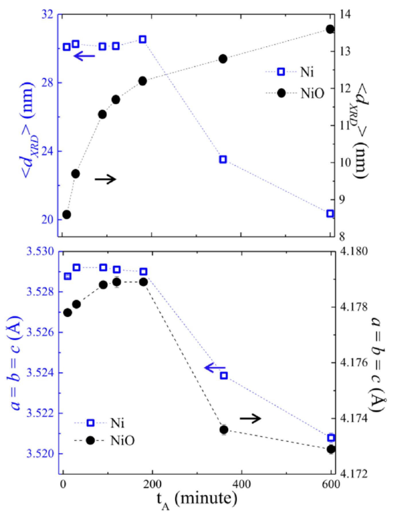
Another similar study concerning the effect of annealing time on the oxidation of Ni nanoparticles has been investigated by Chhaganlal et al. [67]. In this work, a series of Ni/NiO core-shell nanoparticles were synthesized at 300 °C under an ambient atmosphere at different annealing times, indicated as ${\mathrm{t}}_{\mathrm{A}}$, which varies from 10 min to 600 min. From the XRD measurements, the variation of Ni and NiO grain size as a function of ${\mathrm{t}}_{\mathrm{A}}$ was observed. As shown in Figure 12, the Ni grain size stays constant (≈30 nm) below 200 min and drops abruptly from 200 min to 600 min whereas the particle size of NiO slowly varies from 8.6 nm to 13.6 nm, corresponding to an annealing time from 10 to 600 min. The annealing effect on the lattice constants for Ni and NiO is also clearly observed from the lattice constants in Figure 12, which shows lattice contraction for ${\mathrm{t}}_{\mathrm{A}}<200$ min. Finally, it was concluded from the XRD results that the expansion of the NiO shell coincides with the reduction in the Ni core.

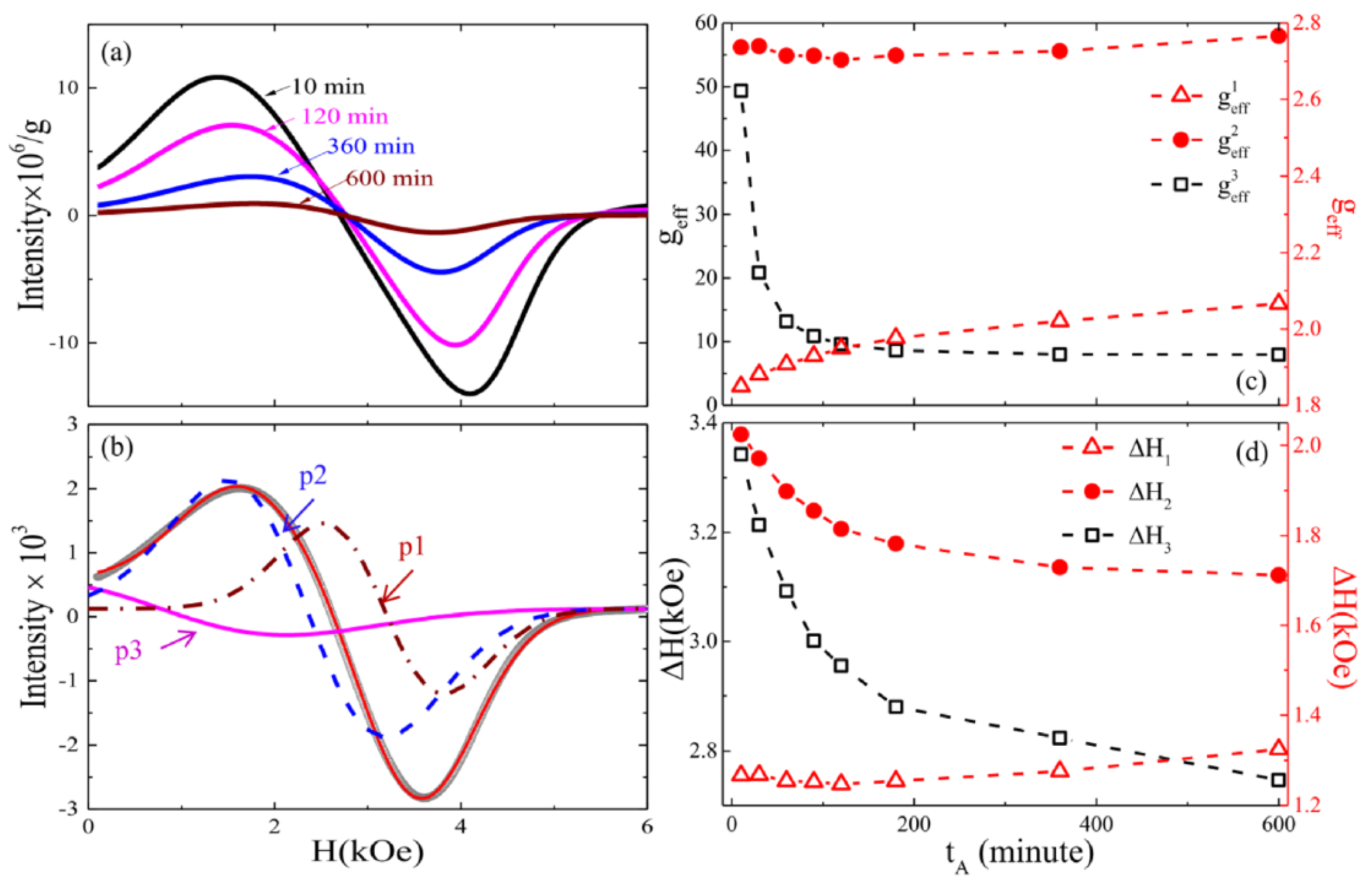
Figure 13a represents the FMR absorption spectra for annealed samples from 10 to 600 min at 300 K. The spectra show both decreasing intensity and line-width with increasing ${\mathrm{t}}_{\mathrm{A}}$. To fit these experimental results, a model was used based on a deconvolution system using the sum of three Gaussian functions [67]:

$$\begin{array}{c}\hfill \frac{dP}{dH}=I_0-\frac{4}{\sqrt{\pi /2}}[a_1\frac{(H-H_{r1})}{\mathsf{\Delta }{H}_1^3}{exp}^{-2{(H-H_{r1})}^2/\mathsf{\Delta }{H}_1^2}\\ \hfill +a_2\frac{(H-H_{r2})}{\mathsf{\Delta }{H}_2^3}{exp}^{-2{(H-H_{r2})}^2/\mathsf{\Delta }{H}_2^2}\\ \hfill +a_3\frac{(H-H_{r3})}{\mathsf{\Delta }{H}_3^3}{exp}^{-2{(H-H_{r3})}^2/\mathsf{\Delta }{H}_3^2}]\end{array}$$

(46)

where $a_1$, $a_2$ and $a_3$ are amplitude, $H_{r1}$, $H_{r2}$ and $H_{r3}$ resonance field and $\mathsf{\Delta }{H}_1$, $\mathsf{\Delta }{H}_2$ and $\mathsf{\Delta }{H}_3$ line-width of $p_1$, $p_2$ and $p_3$ peaks, respectively, as shown in Figure 13b for the sample annealed at 600 min. The use of the deconvolution method with the sum of Gaussian functions allowed a best fit for these samples to be obtained. However, interpreting the results of these fits is also not an easy task. For this, the calculated values of the g-factor and linewidth were plotted as a function of ${\mathrm{t}}_{\mathrm{A}}$. From Figure 13c and for samples with ${\mathrm{t}}_{\mathrm{A}}$ less than 180 min, $g_{eff}^1\approx$ 1.95 can be attributed to the free spins [68]. For samples at 180 min, peak $p_2$ with $g_{eff}^2\approx$ 2.7 and peak $p_3$ with $g_{eff}^3\approx$ 8, Ni nanoparticles and inter-particle interactions are assigned to them, respectively [69]. The decrease in $\mathsf{\Delta }{H}_2$ and $\mathsf{\Delta }{H}_3$ with increasing ${\mathrm{t}}_{\mathrm{A}}$, suggests the reduction in magnetic inhomogeneity.

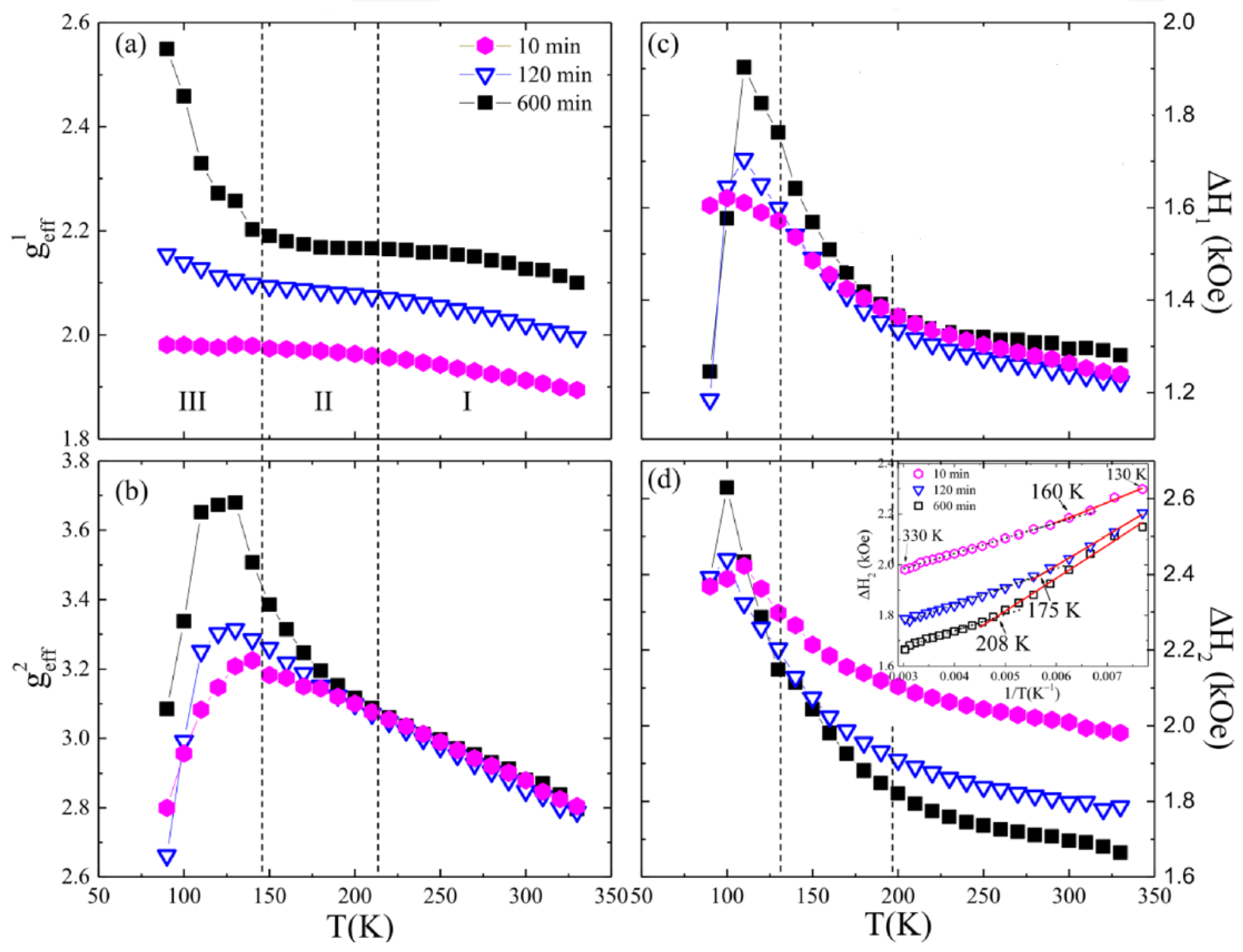
For a more in-depth study, the temperature (T) dependencies of ($g_{eff}^1$, $g_{eff}^2$) and ($\mathsf{\Delta }{H}_1$, $\mathsf{\Delta }{H}_2$) for three typical samples with ${\mathrm{t}}_{\mathrm{A}}$ = 10, 120 and 600 min were measured as displayed in Figure 14. These T dependencies were then analyzed by dividing the data into three regions: $\mathrm{I}$ (330 K–200 K), $\mathrm{II}$ (200 K–130 K), and $\mathrm{III}$ (130 K–90 K). The separation between these regions is delimited by the vertical dotted lines as shown in Figure 11.

In regions $\mathrm{I}$ and $\mathrm{II}$, both $g_{eff}^1$ and $g_{eff}^2$ increase with the decrease in T, which indicates an increase of magnetic interactions. Moreover, the dependence of $g_{eff}^2$ with respect to temperature overlaps for the three samples, while the intensity of $g_{eff}^1$ increases as ${\mathrm{t}}_{\mathrm{A}}$ increases, indicating that the interaction between free spins gets stronger for large size Ni nanoparticles. On the other hand, $g_{eff}^2$ in region $\mathrm{II}$, reaches a peak at ≈130 K with ${\mathrm{t}}_{\mathrm{A}}$ = 600 min. The observed effects may be linked to a rise in effective anisotropy resulting from the emergence of short-range antiferromagnetic (AF) correlations in the NiO particles. This leads to exchange-bias (EB) coupling near the interface of Ni and NiO. Additionally, in region $\mathrm{III}$, there is a significant increase in $g_{eff}^1$ at 600 min, which could be attributed to the long-range AF ordering of NiO. However, $g_{eff}^1$ shows a sudden decline at around 130 K for all the three different ${\mathrm{t}}_{\mathrm{A}}$ values, suggesting again changes in effective anisotropy due to EB coupling.

As the temperature decreases, the linewidth shows a similar behavior to that of the g-factor by increasing in both regions $\mathrm{I}$ and $\mathrm{II}$. The $\mathsf{\Delta }{H}_1$ values of free spins overlap in region $\mathrm{I}$, then begin to separate in region $\mathrm{II}$. At temperatures below 200 K, an increase in $\mathsf{\Delta }{H}_2$ is observed, which is associated with increased anisotropy at low temperatures. To obtain the change of spin relaxation rate, the plot of $\mathsf{\Delta }{H}_2$ versus (1/T) is used, as shown in the inset of Figure 14d. The slope of the curve $\mathsf{\Delta }{H}_2$ (1/T) changes at 208 K, 175 K, and 160 K with respect to ${\mathrm{t}}_{\mathrm{A}}$ = 600, 120, and 10 min, which are approximately the same transition temperatures where $g_{eff}^2$ starts to increase in region $\mathrm{II}$. The observed change in spin relaxation rate is associated with the EB effect at the interface of Ni and NiO.

In order to determine the spin relaxation rate changes, the graph of $\mathsf{\Delta }{H}_2$ as a function of (1/T) is used, as displayed in the inset of Figure 14d. The slope of the $\mathsf{\Delta }{H}_2$ (1/T) curve varies at temperatures of 208 K, 175 K, and 160 K for different values of $t_A$ (600, 120, and 10 min), which approximately correspond to the same transition temperatures at which $g_{eff}^2$ begins to increase in region $\mathrm{II}$. The authors concluded that the observed alteration in spin relaxation rate is linked to the EB effect at the interface of Ni and NiO.

The behavior of magnetic nanoparticles is also determined by their magnetic anisotropy. For this purpose, P. Hernandez-Gomez et al. [70] studied Li ferrite nanoparticles by FMR at different annealing temperatures. These nanoparticles were prepared by the sol-gel technique and then annealed for 4 h in a temperature range from 400 °C to 1000 °C. X-ray diffractograms indicated the particle size increases with annealing temperature, which is in good agreement with the higher crystallinity of the samples induced by the annealing. The $\alpha -{\mathrm{LiFe}}_5{\mathrm{O}}_8$ size varies from (30 ± 3) nm for samples annealed at 400 °C, to (720 ± 26) nm for those annealed at 1000 °C. 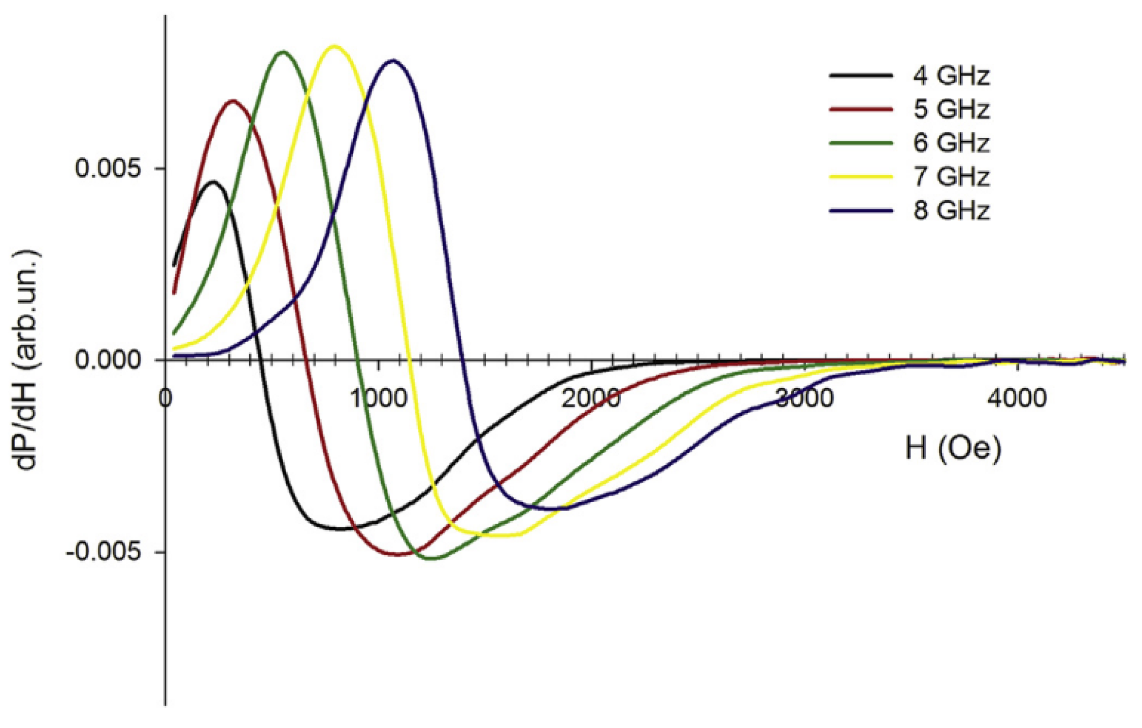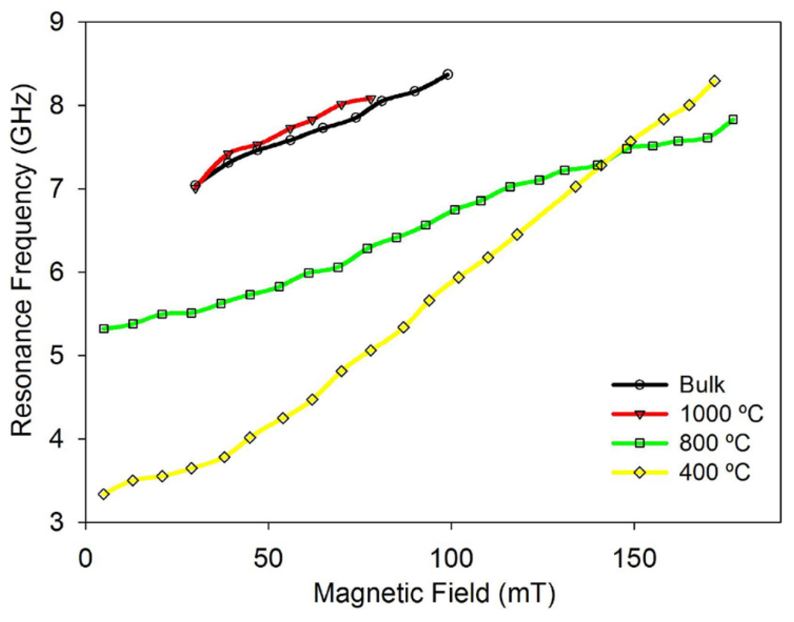Figure 15 shows FMR spectra of Li ferrite nanoparticles at 400 °C annealed temperature with frequencies varying from 4 GHz to 8 GHz where inhomogeneous broadening behavior is observed. This inhomogeneity is common to nanoparticles and can have several origins, such as magnetic inhomogeneities in the sample, random orientations of magnetic anisotropy axis [1], or interaggregate dipolar interaction. By plotting the extracted linewidth as a function of frequency, it is possible to study the damping of the resonance and then identify each damping mechanism contribution. We note that damping can result from both intrinsic and extrinsic contributions [71].

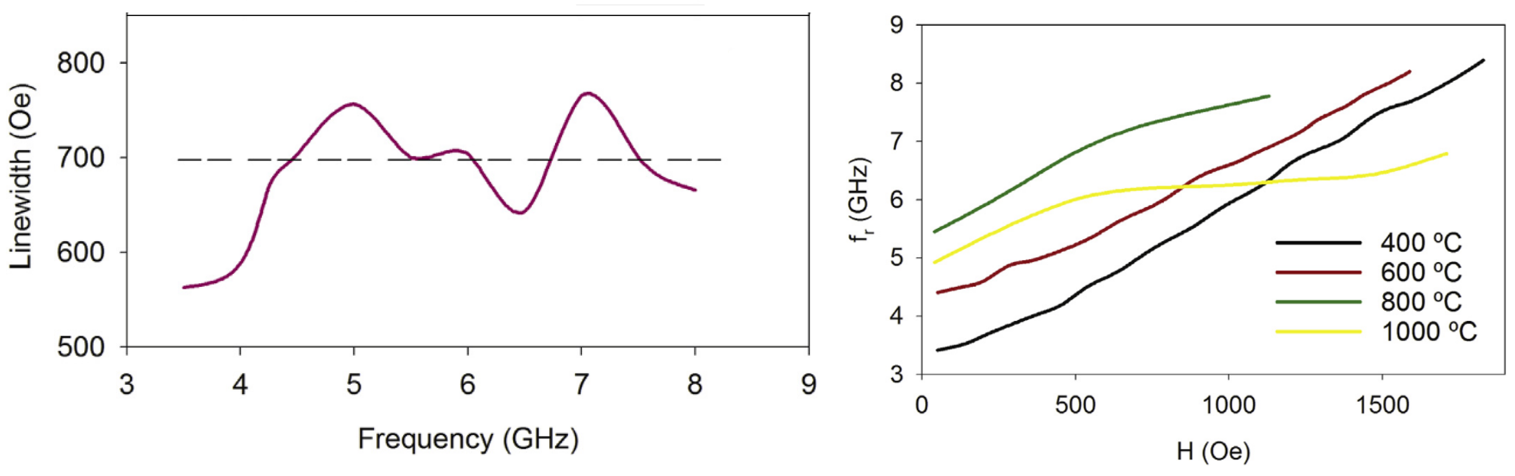
Figure 16 shows the evolution of the linewidth of the sample annealed at 400 °C as a function of frequency. Note that if the Gilbert coefficient is dominant in damping, a linear increase in linewidth with the applied field is observed, which is not the case here. Therefore, it is concluded that in addition to the Gilbert damping parameter, there are dominant extrinsic magnetic relaxation contributions. These contributions would likely come from a high interparticle interaction induced by the aggregation of the nanoparticles; thus, in addition to the dipolar interactions, intracluster exchanges appear, which leads to the observed distorted resonance curve [72].

In order to evaluate the magnetic anisotropy, the dependence of the frequency versus the magnetic resonance field is analyzed as illustrated on the left of Figure 16. This linear dependence is fitted using the Kittel expression:

$$f_r=\frac{\gamma {\mu }_0}{2\pi }.(H_r+H_K)$$

(47)

where $f_r$ is the resonance frequency, $H_r$ the magnetic field at resonance, $\gamma$ is the gyromagnetic ratio, and $H_K$ the effective magnetic anisotropy field. The effective anisotropy values calculated for the samples show a variation, with a value of 1.02 kOe for the sample annealed at 400 °C, and values of 1.42 kOe and 1.92 kOe for the samples annealed at 600 °C and 800 °C, respectively. The anisotropy field is reduced for samples annealed at 1000 °C, which is in good agreement with other spinel ferrite nanoparticles [73].

The saturation magnetization for samples annealed at 1000 °C (${\mathrm{M}}_{\mathrm{s}}=52.7\mathrm{emu}/\mathrm{g}$ ) was measured in order to calculate the value of the effective anisotropy constant $(2.4\pm 0.43)\times {10}^4 \mathrm{J}/{\mathrm{m}}^3$, which is three times higher than the magnetocrystalline anisotropy reported for bulk lithium ferrites [70]. In fact, it is well-known that in the case of nanoparticles, the magnetic anisotropy constant is not only determined by the magnetocrystalline anisotropy but also by other contributions such as surface, strain, shape anisotropy and anisotropy from interparticle interactions, which can explain this increase with respect to the bulk magnetocrystalline anisotropy. Moreover, this value is close to the calculated one ($4.{10}^4\mathrm{J}/{\mathrm{m}}^3$) by Yang et al. [74] who assumed that the nanoparticles annealed at lower temperatures have a core-shell configuration, whereas the larger particles exhibit multidomain behavior. Thus, this anisotropy may also indicate that the Li ferrite nanoparticles are in a core-shell configuration.

A complementary study was carried out by the same authors and by doping Mn in the Li ferrite nanoparticles [75]. Mn-doped Li nanoparticles were prepared under the same conditions as the above-mentioned samples and also annealed in a temperature range between 400 °C and 1000 °C. The extracted FMR data are shown in Figure 17, where the anisotropy magnetic field is obtained by fitting these data using Equation (47). The anisotropy magnetic field lies in the range of 0.9 kOe for samples at 400 °C to 3.30 and 3.70 kOe for annealing temperatures at 800 °C and 1000 °C, respectively. The value of the effective anisotropy constant for sample annealed at 1000 °C was then deduced using ${\mathrm{M}}_{\mathrm{s}}$ measurements (${\mathrm{M}}_{\mathrm{s}}=57\mathrm{emu}/\mathrm{g}$), which gave $(3.75\pm 0.55)\times {10}^4\mathrm{J}/{\mathrm{m}}^3$. This value is also very close to the calculated $4\times {10}^4\mathrm{J}/{\mathrm{m}}^3$) by Yang et al. [74], suggesting a core-shell nanoparticle configuration.

To explain this result, it is important to remember that in polycrystals, Mn substitution reduces grain growth and porosity. This is confirmed by the fact that the average nanoparticle size in Mn-doped Li ferrite samples annealed at 1000 °C is lower than that of undoped Li ferrite samples annealed for the same temperature, with a size of 205 nm compared to 720 nm, respectively. Moreover, Mn cations can impede the presence of ferrous cations; thus, ${\mathrm{Mn}}^{2+}$ and ${\mathrm{Mn}}^{3+}$ are present, where it (${\mathrm{Mn}}^{3+}$) can modify the local crystal fields, and consequently, the anisotropy constant [76]. Furthermore, it is also well-established that Mn addition in Li ferrites significantly reduces the magnetostriction constants [77].

FMR was also used to investigate the annealing effect on Nickel Cobal ferrite nanoparticles [78]. ${\mathrm{Ni}}_{0.4}{\mathrm{Co}}_{0.6}{\mathrm{Fe}}_2{\mathrm{O}}_4\left(NCF\right)$ nanoparticles were prepared using the solvothermal method, known as a simple and inexpensive technique for preparing ferrite nanoparticles at low temperatures [79]. A portion of these samples was then annealed for 5 h at 1000 °C and will be referred to as an-NCF nanoparticles, whereas the as-prepared NiCo ferrite nanoparticles are referred to as ap-NCF.

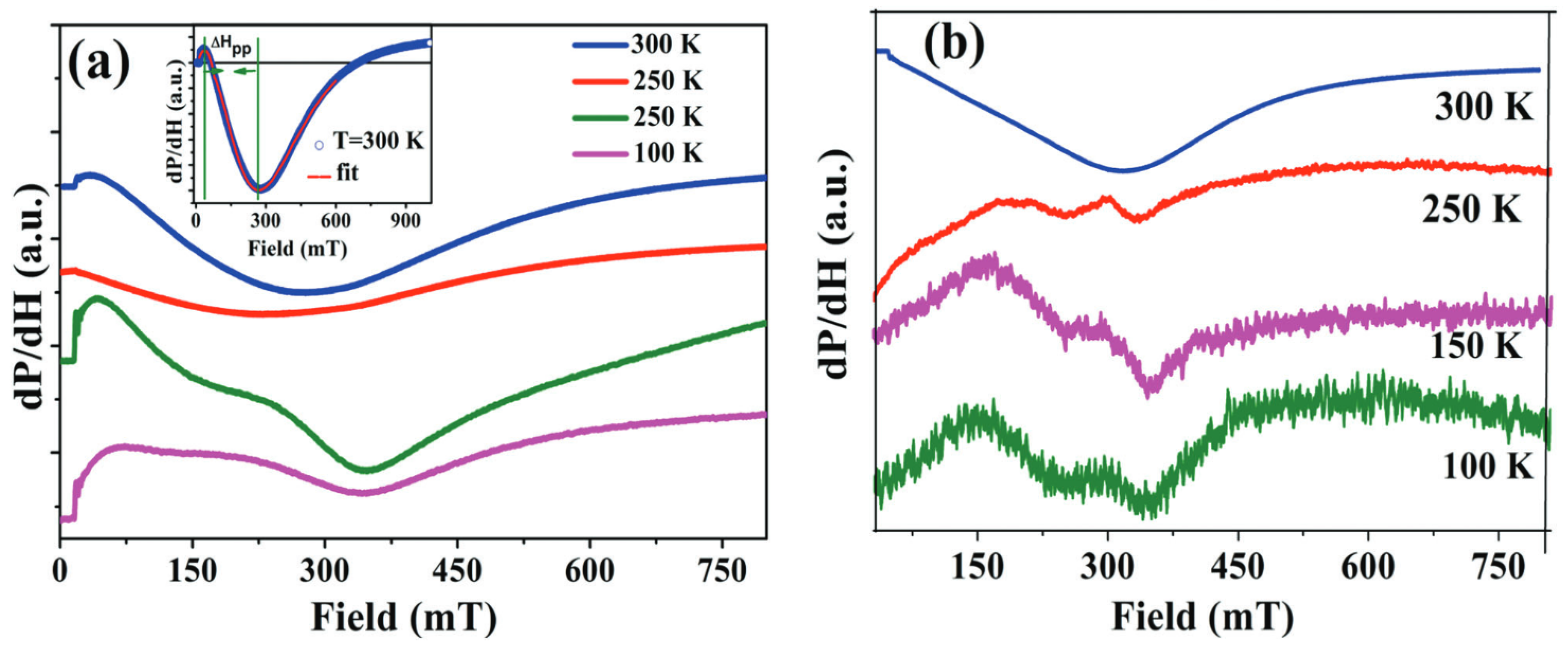
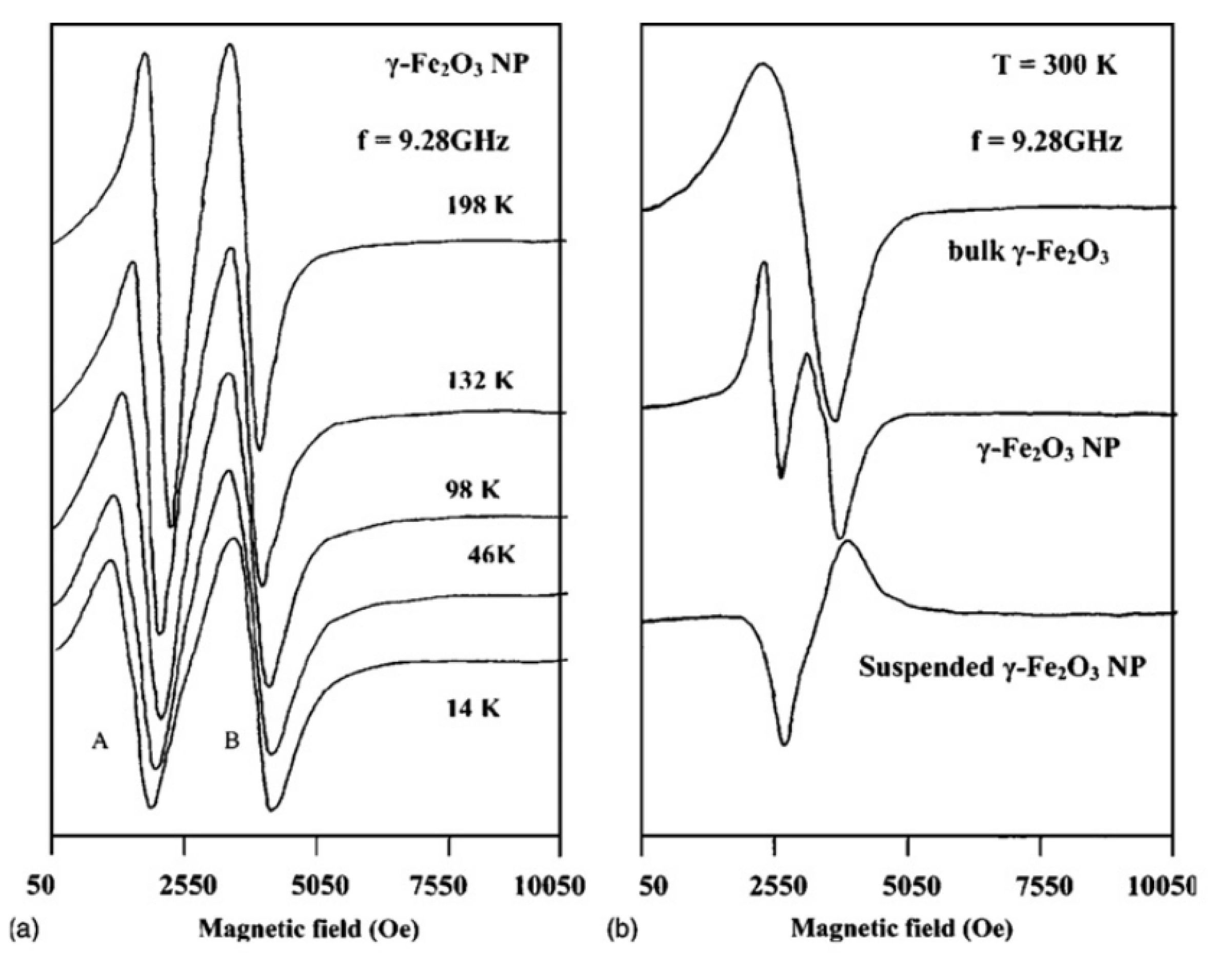
FMR measurements of NCF nanoparticles were performed over a temperature range between 100 K and 300 K. These FMR curves are illustrated in Figure 18 and show an asymmetric and inhomogeneous line shape. In addition, the FMR spectra indicate the presence of two distinct resonance lines that merge into a single broad resonance line at temperatures exceeding 250 K. Multipeaked spectra are common in FMR studies with nanoparticles and have been observed by other authors such as for $\gamma -{\mathrm{Fe}}_2{\mathrm{O}}_3$, illustrated in Figure 19, which was measured by Dutta et al. [80]. It should be noted that additional resonances can also be observed in FMR experiments for nanoparticles, typically due to surface effects and inhomogeneities in the assembly.

The FMR spectra in Figure 18 were then fitted using Gaussian curve [81] as displayed in the inset of Figure 18a for a representative sample of ap-NCF at 300 K. The obtained resonance field ($H_r$), peak-to-peak linewidth ($\mathsf{\Delta }{H}_{PP}$) and g-factor are summarized in

Table 2. The extracted FMR variables of ap-NCF and an-NCF nanoparticles at different temperatures after fitting FMR curves using Gaussian model [78,81]. Table reprinted with permission from G. Datt, C. Kotabageb and A. C. Abhyankar, Ferromagnetic resonance of NiCoFe₂O₄ nanoparticles and microwave absorption properties of flexible NiCoFe₂O₄—carbon black/poly(vinyl alcohol) composites, Phys. Chem. Chem. Phys., 19, 20699. Copyright (2017) ROYAL SOCIETY OF CHEMISTRY.

	ap-NCF			an-NCF
Temp (K)	${\mathit{H}}_{\mathit{r}}$(Oe)	$\mathsf{\Delta }{\mathit{H}}_{\mathit{PP}}$(Oe)	${\mathit{g}}_{\mathit{eff}}$	${\mathit{H}}_{\mathit{r}}$(Oe)	$\mathsf{\Delta }{\mathit{H}}_{\mathit{PP}}$(Oe)	${\mathit{g}}_{\mathit{eff}}$
100	1700	2700	3.78	2350	2000	3.73
150	2000	3000	3.21	2450	1820	2.62
250	1300	2300	4.94	2550	1400	2.51
300	1400	2900	4.59	2500	2700	2.57

. From Table 2, it can be noted that the values of the g-factor and linewidth are higher for the ap-NCF samples than in an-NCF samples, unlike the resonance field, which is higher for an-NCF nanoparticles.

To discuss these findings, it should be remembered that the FMR condition resonance can be expressed as $\omega =\gamma H_{eff}$, where $\omega$, $\gamma$, and $H_{eff}$ represent the resonance frequency, gyromagnetic ratio, and effective magnetic field, respectively. $H_{eff}$ is composed of various contributions, such as magnetic anisotropy field ($H_K$) exchange interaction field ($H_{ex}$), demagnetization field ($H_D$), and dipole–dipole interactions (see Section 4.2). For strongly coercive magnets, $H_D$ and dipole–dipole interaction effects can be ignored. $\mathsf{\Delta }{H}_{PP}$, depends on the exchange interaction and the magnetic anisotropy and can be represented by $\mathsf{\Delta }{H}_{PP}\approx H_K^2/H_{ex}$. Thus, this expression indicates that the magnetic anisotropy broadens $\mathsf{\Delta }{H}_{PP}$ while the exchange interaction narrows it. In addition, $H_K$ is determined by the effective anisotropy constant, $K_{eff}$, as $H_K=2K_{eff}/M_s$. $K_{eff}$ is calculated using the diameter D of a spherical nanoparticle and is expressed as $K_{eff}=K_b+(6/D)K_s$, where $K_b$ and $K_s$ represent the bulk and surface anisotropy constants, respectively. This means that anisotropy is enhanced for smaller nanoparticles due to the factor of 6/D. On the other hand, Mossbauer studies have shown that the exchange interactions in ap-NCF nanoparticles are weaker than those in an-NCF nanoparticles because of broken bonds at large surfaces [82]. The disorder on the surface for ap-NCF nanoparticles results in a decrease in $H_{ex}$, increasing $H_K$ and thus broadening $\mathsf{\Delta }{H}_{PP}$. In contrast, an-NCF nanoparticles are octahedral and arrange magnetic domains along different facets to reduce surface anisotropy. Moreover, annealing at 1000 °C reduces cationic disorder (which refers to the randomness or irregularity in the arrangement of cations in a crystal structure) and enhances exchange interaction among crystallites, consequently resulting in a decrease in the FMR linewidth for an-NCF nanoparticles.

For the resonance field, it is noteworthy that the ap-NCF nanoparticles exhibit a significantly higher $g_{eff}$ with a significantly smaller $H_r$ up to 300 K, as per the equation: $g_{eff}=h\nu /{\mu }_B{H}_r$, where ${\mu }_B$ is the Bohr magneton and $\nu$ = 9.27 GHz, the frequency used for recording FMR spectra.

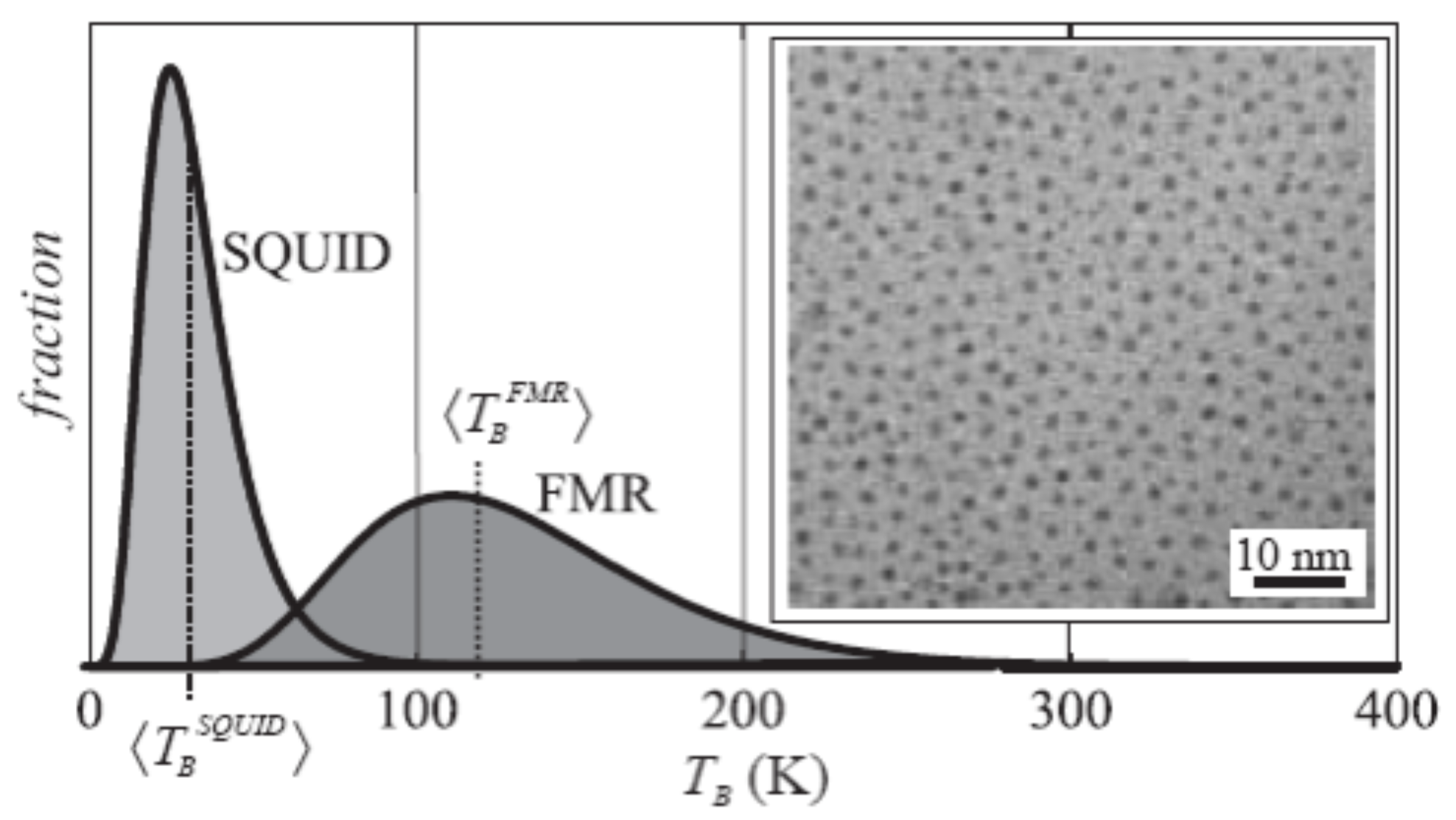
The magnetic behavior of nanoparticles is significantly influenced by the temperature dependence of the magnetic anisotropy. Antoniak et al. [49] conducted a study where the used both FMR and SQUID data to evaluate ${\tau }_0$ and $K_{eff}$ in FePt nanoparticles from two different blocking temperatures for these methods. The analysis of the FMR data was performed using the Kittel equation:

$${\left(\frac{\omega }{\gamma }\right)}^2=\left[H_{\mathrm{res}}cos(\vartheta -\theta )+H_{K}cos2\vartheta \right]\left[H_{res}cos(\vartheta -\theta )-H_K{cos}^2\vartheta \right]$$

(48)

where $H_K=2K_{eff}/M_s$ is the effective anisotropy field including the uniaxial contribution resulting from minor deviations from a spherical shape, surface, and step anisotropies present at the particle surface that are not averaged. Averaging of the external magnetic field angles ${\phi }_H$ gives:

$$H_{\mathrm{res}}=H_{\mathrm{res}}^0{\left[1-{\left(\frac{H_K}{H_{\mathrm{res}}^0}\right)}^{1.25}\right]}^{0.44}$$

(49)

where $H_{res}^0=\hslash \omega /g{\mu }_0{\mu }_B$ gives g-factor as 2.054 ± 0.010. The blocking temperature was evaluated by analyzing the intensity versus temperature, as the intensity of the FMR line is proportional to the magnetization. However, the blocking temperature evaluated using this method is expected to be higher than that obtained from SQUID measurements due to the significant difference in the time windows of the two methods; ${\tau }_{FMR}\approx {10}^{-10}$ s and ${\tau }_{SQUID}\approx {10}^2$ s. 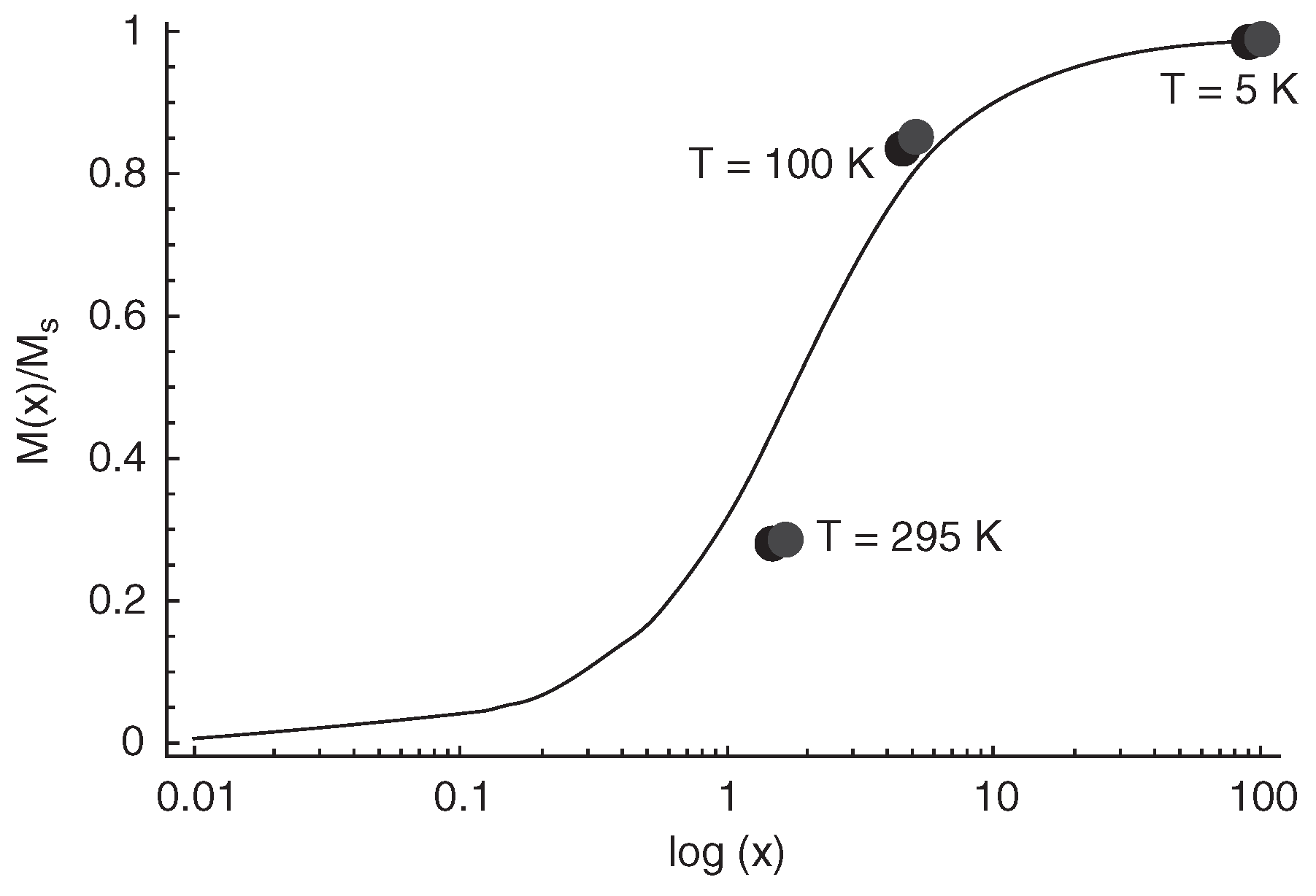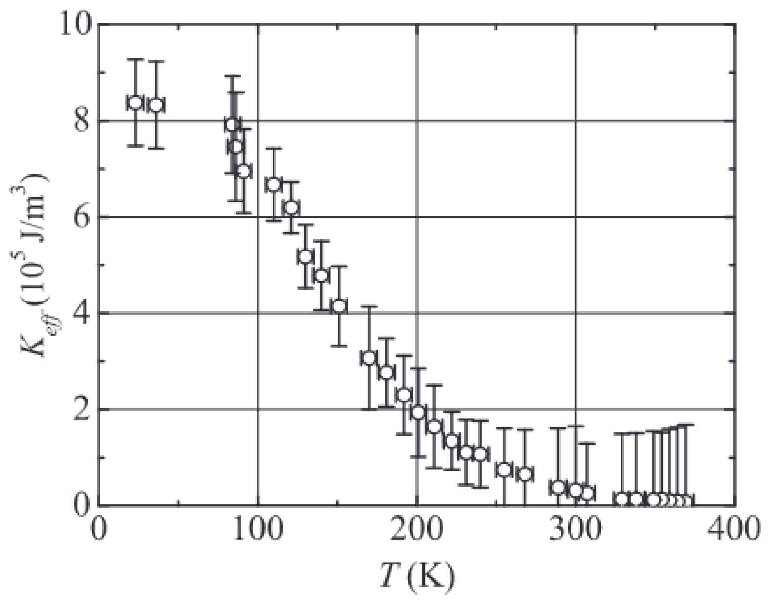By comparing the two blocking temperatures, as shown in Figure 6 and applying the Arrhenius relationship, the expression of the effective anisotropy can be expressed in the form:

$$K_{\mathrm{eff}}\left(〈T_B^{SQUID}〉\right)\approx \frac{27k_B}{V_m}{\left[\frac{1}{〈T_B^{SQUID}〉}-\frac{\alpha }{〈T_B^{FMR}〉}\right]}^{-1}$$

(50)

where $\alpha =H_K\left(〈T_B^{FMR}〉\right)/H_a\left(〈T_B^{SQUID}〉\right)$ and $V_m$ is the mean volume. From this equation and using $\alpha =$ 0.8 and $〈T_B^{FMR}〉$ = 110 K, it was found that $K_{eff}$ = ($8.4\pm 0.9)\times {10}^5\mathrm{J}.{\mathrm{m}}^{-3}$ at 23 K (as shown in Figure 20) and ${\tau }_0\approx 1.7\times {10}^{-12}$ s. The experimental data reveals that the values of $K_{eff}$ follow a Bloch law-like relationship with a power of 2.1, described as $K_{eff}$ proportional to ${\left[M_s{(1-T/T_B)}^{3/2}\right]}^{2.1}$ [49]. The anisotropy in this sample was discovered to be roughly ten times higher than that observed in the bulk.

5.2. Doping Effect

The use of ferromagnetic resonance to study the effects of doping on the properties of the magnetic nanoparticles is of great importance due to the potential applications of these materials in various fields, such as biomedicine and data storage. Doping, which consists of the introduction of impurities, can alter, in addition to the electrical and optical properties, the magnetic properties of nanoparticles, including their magnetic moment, magnetic anisotropy, etc. Indeed, magnetization is strongly dependent on the distribution of different ions on the different sites of the crystal lattice. Thus, understanding how different dopants affect these properties can lead to the development of more efficient and versatile magnetic nanoparticles depending on the targeted applications.

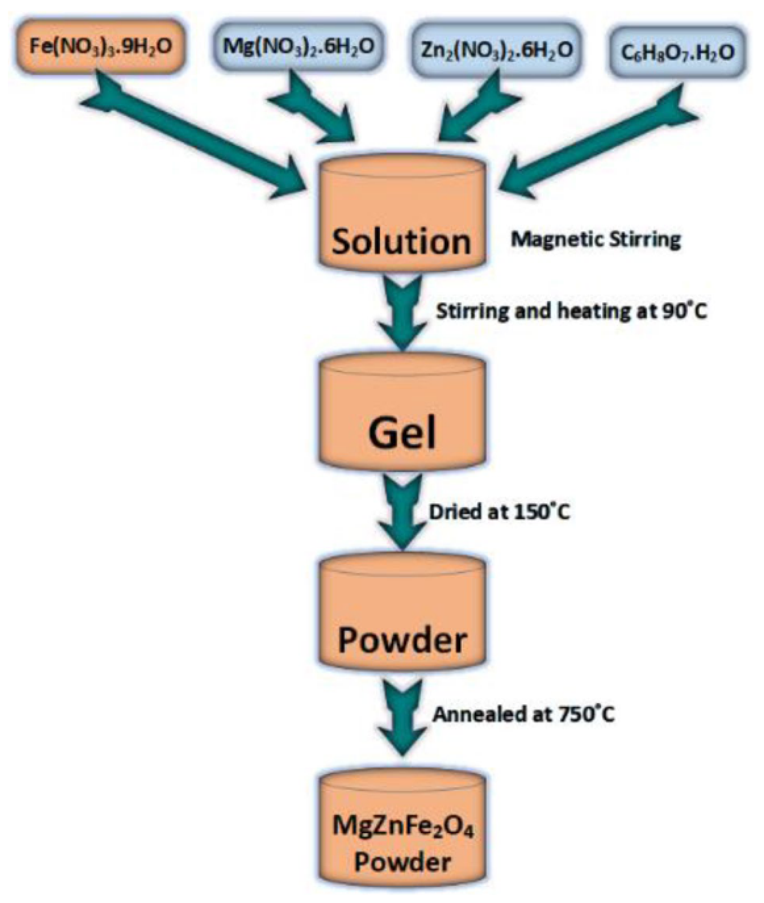
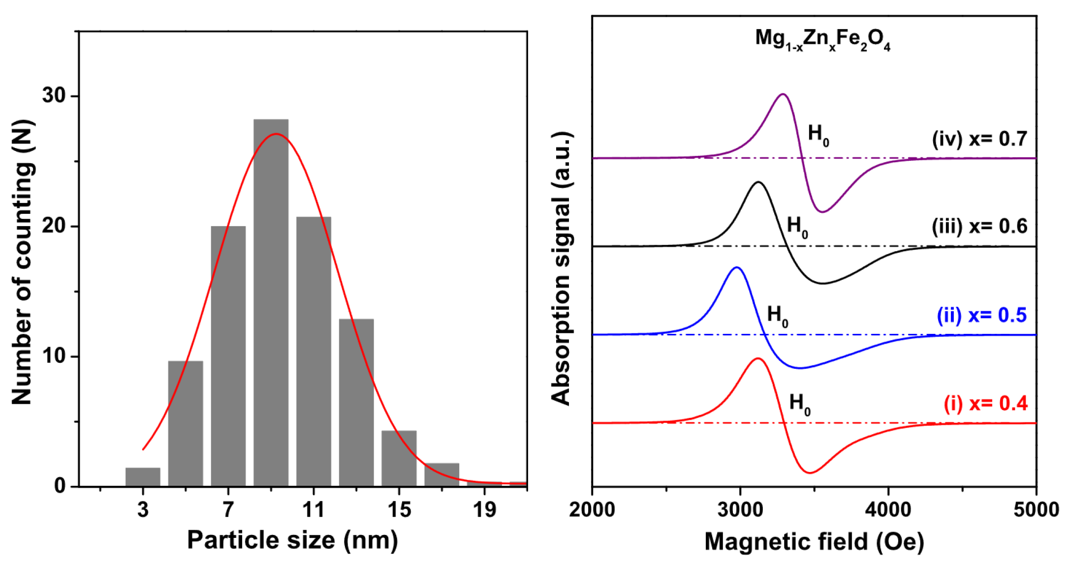
The study of the influence of changes in chemical composition by introducing Zn content in ${\mathrm{Mg}}_{1-\mathrm{x}}{\mathrm{Zn}}_{\mathrm{x}}{\mathrm{Fe}}_2{\mathrm{O}}_4$ nanoparticles (x = 0.4, 0.5, 0.6, 0.7) were studied by Tsay et al. [83]. These nanoparticles were synthesized using the hydrothermal method. XRD data allowed an estimation of the average nanocrystallite sizes $(7.75\pm 0.03)$ nm to $(9.28\pm 0.04)$ nm, which was consistent (9 nm to 10.3 nm) with data extracted from TEM images as shown in Figure 21 (left).

The FMR spectra of the Mg-Zn ferrite nanoparticles are plotted in Figure 21, from which the values of resonance field ($H_r$) g-factor and linewidth are obtained and given in

Table 3. FMR characteristics of ${\mathrm{Mg}}_{1-\mathrm{x}}{\mathrm{Zn}}_{\mathrm{x}}{\mathrm{Fe}}_2{\mathrm{O}}_4$ nanoparticles. Reprinted with permission from Tsay Chien-Yie, Chiu Yi-Chun and Tseng Yung-Kuan, Investigation on structural, magnetic, and FMR properties for hydrothermally-synthesized magnesium-zinc ferrite nanoparticles, Physica B: Condensed Matter, 570, 29. Copyright (2019) Elsevier.

Zn Content (x)	${\mathit{H}}_{\mathit{r}}$ (Oe)	$\mathbf{\Delta }\mathit{H}$ (Oe)	G-Factor
x = 0.4	3295	350	2.14
x = 0.5	3166	350	2.23
x = 0.6	3317	435	2.13
x = 0.7	3418	265	2.06

. For these nanoparticles, the g-factor and resonance field varied independently of the Zn content, unlike the linewidth, which increases as a function of Zn content up to x = 0.6 before significantly decreasing to 265 Oe for x = 0.7. On closer inspection, it is observed that the FMR line is not symmetrical (particularly for x = 0.4, 0.5, and 0.6), which could also distort the measurements of the linewidth. However, these linewidth values compared to other ferrite nanoparticles are narrower, suggesting a lower magnetic loss and a better magnetic field homogeneity [84].

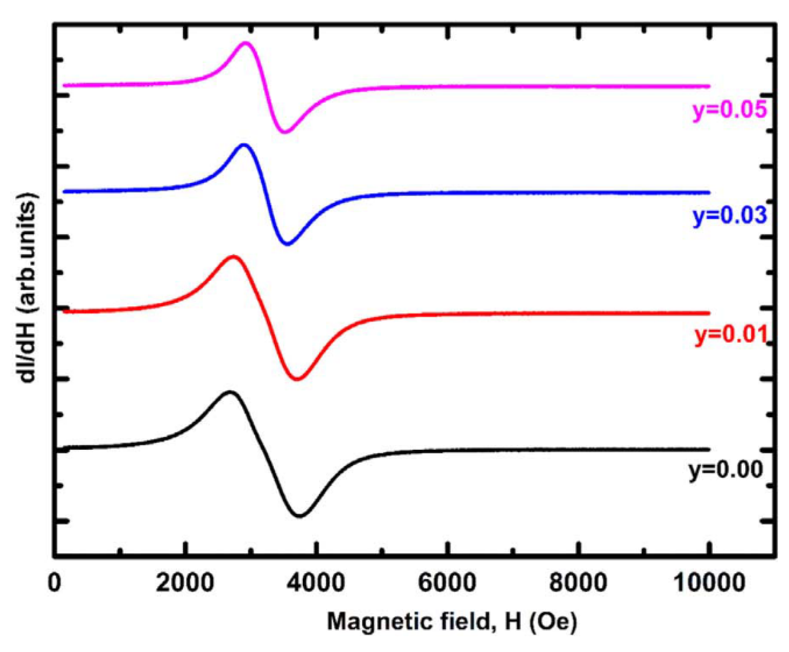
The doping of nonmagnetic ions in Mg-Zn ferrite nanoparticles such as scandium (Sc) was investigated for the first time by Angadi et al. [85]. They synthesized ${\mathrm{Sc}}^{3+}$-doped ${\mathrm{Mn}}_{0.5}{\mathrm{Zn}}_{0.5}{\mathrm{Sc}}_{\mathrm{x}}{\mathrm{Fe}}_{2-\mathrm{x}}{\mathrm{O}}_4$ (x = 0.00, 0.01, 0.03, and 0.05) nanoparticles using solution combustion method.

Dynamic magnetic properties have been investigated using FMR at 9.1 GHz, where the obtained spectra are represented in Figure 22. The value of $H_r$, $\mathsf{\Delta }{H}_{pp}$, and g-factor are summarized in

Table 4. Effect of the Sc-doped Mn-Zn ferrite nanoparticles on the resonance field ($H_r$), peak-to-peak FMR linewidth $\mathsf{\Delta }{H}_{pp}$ and g-factor. Reprinted with permission from V. Jagdeesha Angadi et al., Structural, electrical and magnetic properties of ${\mathrm{Sc}}^{3+}$-doped Mn-Zn ferrite nanoparticles, Journal of Magnetism and Magnetic Materials, 424, 1–11. Copyright Elsevier (2017).

Sc Content (x)	${\mathit{H}}_{\mathit{r}}$ (Oe)	$\mathbf{\Delta }{\mathit{H}}_{\mathit{PP}}$ (Oe)	G-Factor
x = 0.00	3211	987	2.25
x = 0.01	3265	936	2.19
x = 0.03	3211	670	2.11
x = 0.05	3211	603	2.05

. While the resonance field shows no correlation with the Sc composition, the peak-to-peak linewidth decreases with increasing Sc. Note that the values of $\mathsf{\Delta }{H}_{pp}$ for x = 0.00 and x = 0.01 are very close, as it is also the case for x = 0.03 and x = 0.05. Moreover, considering the FMR lines in Figure 22, it appears that it is composed of two resonances very close to each other (x = 0.00 and x = 0.01), which merge from x = 0.03. This can also explain the drop of $\mathsf{\Delta }{H}_{pp}$ between x = 0.01 and x = 0.03 and the broadening of the FMR line for these two samples.

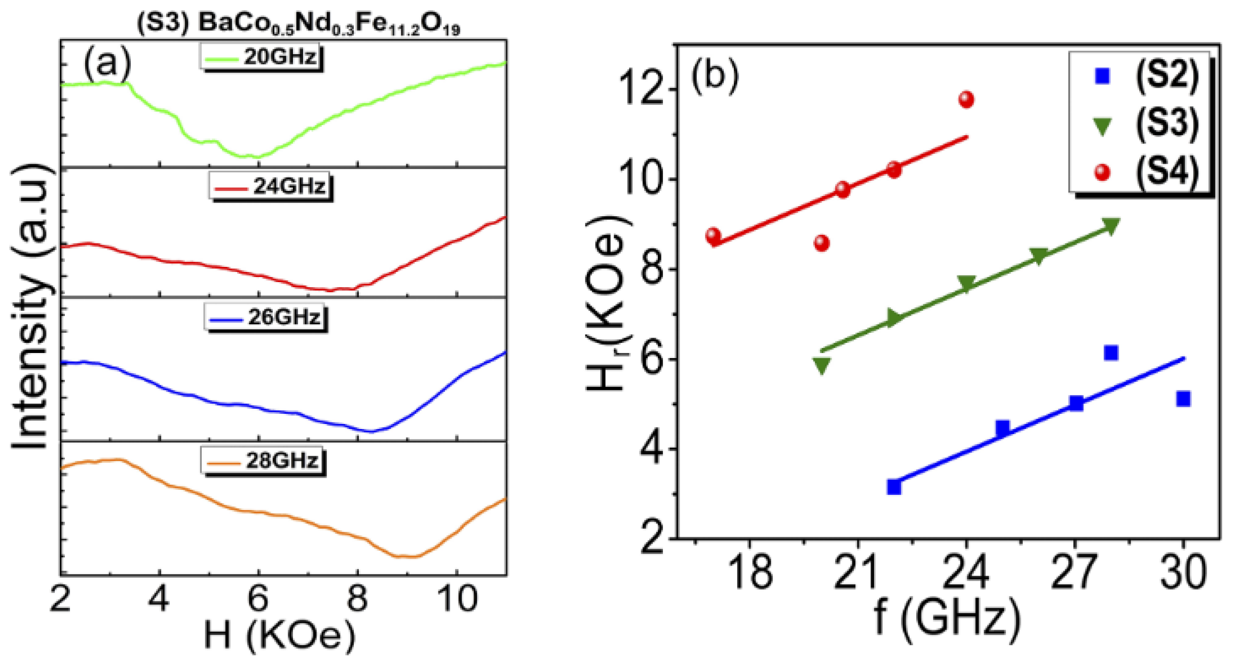
FMR can also be employed to investigate how the use of multiple dopants affects the magnetic properties of nanoparticles. For this purpose Sharma et al. [86] prepared a series of samples based on barium hexaferrite nanoparticles doped with cobalt (Co), samarium (Sm), and neodymium (Nd). The obtained samples are identified as S1 (${\mathrm{BaFe}}_{12}{\mathrm{O}}_{19}$), S2 (${\mathrm{BaCo}}_{0.5}{\mathrm{Fe}}_{11.5}{\mathrm{O}}_{19}$), S3 (${\mathrm{BaCo}}_{0.5}{\mathrm{Nd}}_{0.3}{\mathrm{Fe}}_{11.2}{\mathrm{O}}_{19}$), and S4 (${\mathrm{BaCo}}_{0.5}{\mathrm{Sm}}_{0.3}{\mathrm{Fe}}_{11.2}{\mathrm{O}}_{19}$).

FMR measurements were performed in field sweep mode as shown in Figure 23a for sample S3. The extracted $H_r$ values were then plotted as a function of frequency as illustrated in Figure 23b, where it can be inferred that the Sm-doped hexaferrite (S4) exhibits the highest resonance field at a specific frequency, whereas sample S2 (without Nd or Sm substitution) shows the lowest resonance field. The experimental data in Figure 23b can be fit using a spherical nanoparticle model where the effective magnetic field and the resonance field are given by:

$$H_{eff}=H_D+H_a+H_{int}$$

(51)

$$H_r=\frac{\omega }{\gamma }-H_{eff}=\frac{2\pi f}{\gamma }-H_{eff}$$

(52)

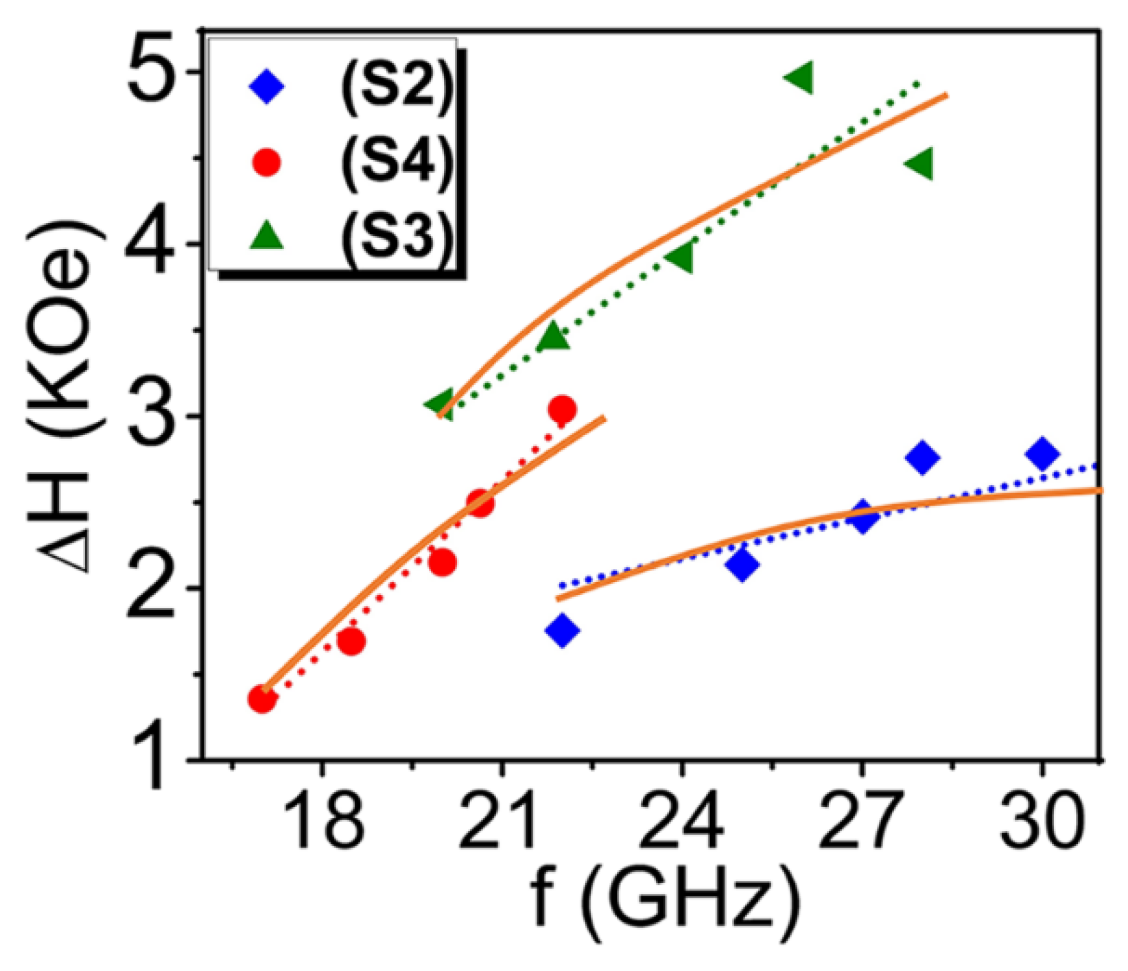
where $H_{int}$ is the interparticle interaction field and $\omega =2\pi f$ the Larmor precession frequency. The author did not give more details on the fitting parameters, nor on the deduced values of ${\mathrm{H}}_{\mathrm{a}}$, for example. However, the measurement of the linewidth (shown in Figure 24) has been well developed. The experimental data of $\mathsf{\Delta }H$ Vs. frequency was first fitted using the Landau–Lifshitz–Gilbert (LLG) damping model:

$$\mathsf{\Delta }H=\mathsf{\Delta }{H}_0+\frac{2}{\sqrt{3}}\left(\frac{4\pi \alpha f}{\gamma {\mu }_0}\right)$$

(53)

where $\alpha$ is the Gilbert damping parameter and $\mathsf{\Delta }{H}_0$ is the inhomogeneous contribution to the linewidth. The application of Equation (53) yields a linear relationship between linewidth and frequency (dotted lines in Figure 24). However, upon careful examination of experimental $\mathsf{\Delta }H$ values, it was observed that the high-frequency values exhibit a downward curvature. In order to explain this behavior in the high-frequency region, a nonlinear model proposed by Bastrukov et al. [87] was used to fit the data points (solid lines in Figure 24). Thus, the modified LLG model:

$$\mathsf{\Delta }H=\frac{4\pi f}{{\gamma }^{{}^{\prime }}{\mu }_0}[{\alpha }^{{}^{\prime }}-{\beta }^{{}^{\prime }}(1-{\left(\frac{\gamma {\mu }_0{M}_s}{2\pi f}\right)}^{1/2})]$$

(54)

where ${\alpha }^{{}^{\prime }}$ is the intrinsic contribution to damping (the Gilbert parameter), and ${\beta }^{{}^{\prime }}$ represents the overall extrinsic contributions to damping such as defects or inhomogeneities in the nanoparticles system.

Table 5. FMR Linewidth parameters using LLG (Equation (53)) and LLG modified (Equation (54)) model [86]. Reprinted from V. Sharma, S. Kumari, and B. K. Kuanr, Rare earth-doped M-type hexaferrites; ferromagnetic resonance and magnetization dynamics, AIP Advances, 8, 056232. Open access (2018) AIP Publishing. Creative Commons Attribution (CC BY) license, https://creativecommons.org/licenses/by/4.0/, accessed on 10 July 2023.

	LLG Model			Modified LLG Model
Sample	$\mathsf{\Delta }{\mathit{H}}_{\mathbf{0}}$(kOe)	$\mathit{\alpha }(\times {\mathbf{10}}^{-\mathbf{2}})$	$\mathit{\gamma }$(GHz/kOe)	${\mathit{\alpha }}^{{}^{\prime }}(\times {\mathbf{10}}^{-\mathbf{2}})$	${\mathit{\beta }}^{{}^{\prime }}(\times {\mathbf{10}}^{-\mathbf{2}})$	${\mathit{\gamma }}^{{}^{\prime }}$(GHz/kOe)
${\mathrm{BaCo}}_{0.5}{\mathrm{Fe}}_{11.5}{\mathrm{O}}_{19}$	1.53	3.48	2.89	1.76	2.58	2.79
${\mathrm{BaCo}}_{0.5}{\mathrm{Nd}}_{0.3}{\mathrm{Fe}}_{11.2}{\mathrm{O}}_{19}$	0.76	5.56	2.86	1.36	6.11	2.84
${\mathrm{BaCo}}_{0.5}{\mathrm{Sm}}_{0.3}{\mathrm{Fe}}_{11.2}{\mathrm{O}}_{19}$	4.32	7.61	2.91	6.14	3.45	2.90

shows the obtained FMR parameters after fitting data in Figure 24 by Equation (53) and (54).

From the Table 5, the LLG model reveals that the highest $\mathsf{\Delta }{H}_0$ was measured for sample S4, where $\alpha$ increases from $3.48\times {10}^{-2}$ for sample S2 to $7.61\times {10}^{-2}$ for sample S4. Indeed, the steepness of the line for S4 in Figure 24 is due to the slope of ($\alpha /\gamma$) being 0.026 for S4, whereas it is half this value (0.012) for S2. The value of $\gamma$ remains unchanged by doping. In the same way, using the modified LLG model, ${\alpha }^{{}^{\prime }}$ Gilbert damping was found to increase from $1.76\times {10}^{-2}$ for sample S2 to $6.14\times {10}^{-2}$ for sample S4, while the extrinsic damping coefficient (${\beta }^{{}^{\prime }}$) was highest for sample S3 ($6.11\times {10}^{-2}$) and lowest for the sample S2 ($2.58\times {10}^{-2}$). These observations allow us to conclude that Nd or Sm ion substitution in Barium hexaferrite induces an increase in the Gilbert damping parameter.

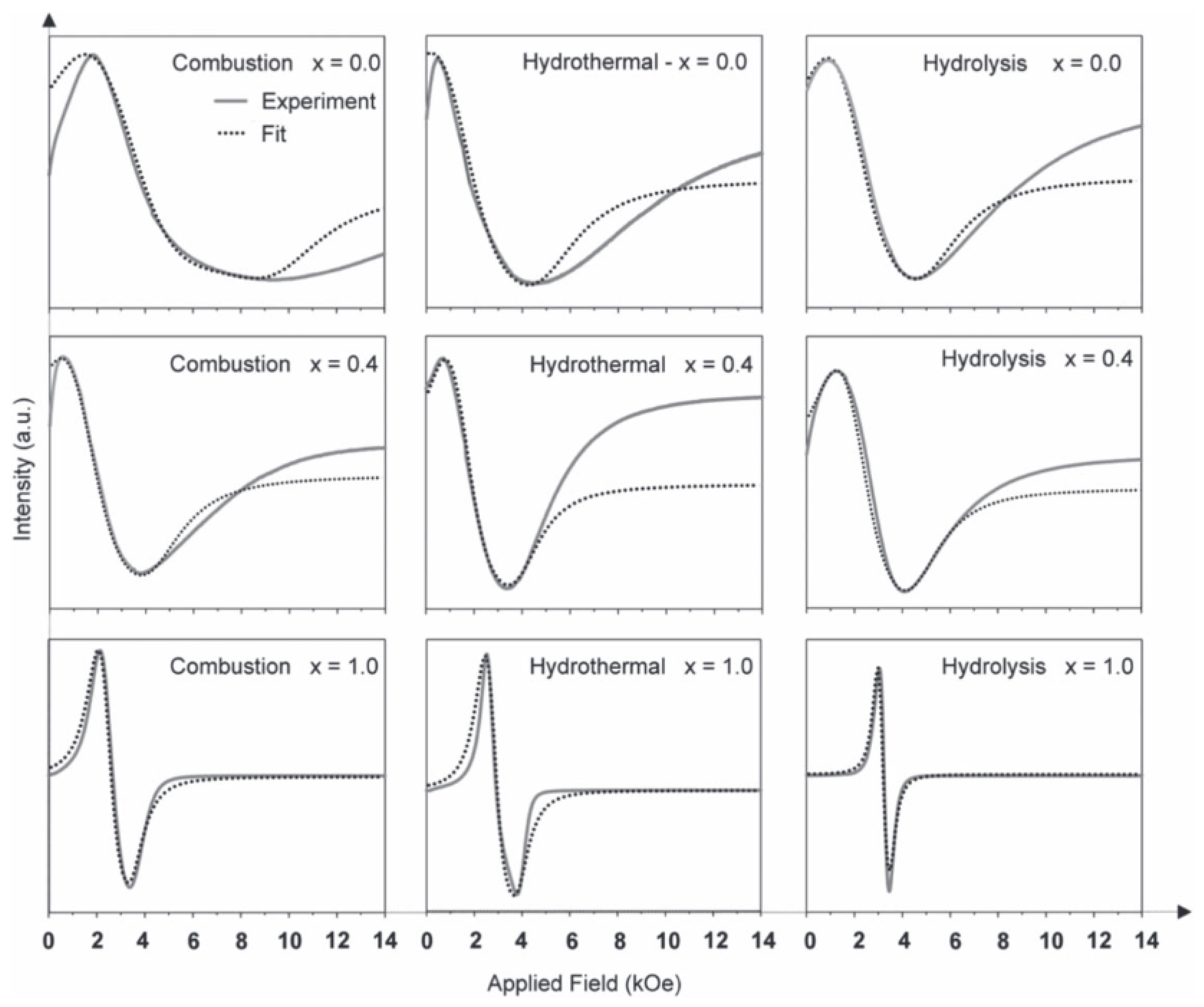
In another study, Pessoa et al. [14] used different synthesis techniques to produce iron-based mixed cubic ferrites ${\mathrm{Co}}_{1-\mathrm{x}}{\mathrm{Ni}}_{\mathrm{x}}{\mathrm{Fe}}_2{\mathrm{O}}_4$ (x = 0.0, 0.4 and 1.0). These nanoparticles were synthesized by hydrothermal (HT), forced hydrolysis (FH), and combustion (C) methods [14]. From the X-ray measurements, a large difference in the average grain size was observed depending on the synthesis method. The FH method, for example, resulted in nanoparticles with a lower degree of crystallinity and average grain size below 10 nm as shown in

Table 6. Parameters obtained from FMR spectra fitting using the model proposed by Tsay et al. [14,65]. Reprinted with permission from M.S. Pessoa, P.S. Moscon, R.S. Melo, A.Jr. Franco, and P.C. Morais, A comprehensive study of ${\mathrm{Co}}_{1-\mathrm{x}}{\mathrm{Ni}}_{\mathrm{x}}{\mathrm{Fe}}_2{\mathrm{O}}_4$ nanoparticles fabricated via three different synthetic methods, Mater. Res. Express, 6, 125068. Copyright (2019) IOP Publishing.

	D (nm)			G-Factor			${\mathit{H}}_{\mathit{K}}$ (Oe)			$\mathbf{\Delta }{\mathit{H}}_{\mathit{PP}}$ (Oe)
x	C	HT	FH	C	HT	FH	C	HT	FH	C	HT	FH
0.0	52	16	8.9	1.5	3.25	2.65	−4600	−2445	−2165	7660	4075	3610
0.4	35	36	9.3	3.35	3.40	2.65	−1968	−1620	−1660	3280	2700	2765
1.0	33	80	5.5	2.62	2.32	2.19	−747	−769	−252	1245	1282	420

.

FMR measurements were carried out at room temperature for all the samples in order to investigate their magnetic anisotropy. The measured FMR spectra are shown in Figure 25, where the solid lines represent experimental data whereas the dotted lines represent the fits using the model proposed by Tsay et al. [65]. Table 6 summarizes the resulting values of the peak-to-peak linewidth ($\mathsf{\Delta }{H}_{PP}$), the magnetic anisotropy field ($H_K$), and the g-factor. For the same synthesis method, Figure 25 shows an increase in the FMR spectra symmetry as a function of increasing x, which allows a better fit.

Table 6 highlights a noteworthy trend, where the peak-to-peak linewidth decreases with the increase in nickel content (x). This is in good agreement with a better fit of the FMR lines for x = 1. It also aligns with the fact that nickel ferrites (x = 1) have a smaller absolute value of crystalline anisotropy than cobalt ferrites (x = 0), as shown by the extracted magnetocrystalline anisotropy field in Table 6. Indeed, as the magnetocrystalline anisotropy field value increases, the external magnetic field becomes stronger and able to sweep the anisotropy from the [111] direction to the [100] direction, which corresponds to the larger (positive) and smaller (negative) crystalline anisotropy, respectively [64]. It should also be noted that the FH method gives samples with the lowest $H_K$ and $\mathsf{\Delta }{H}_{PP}$ values.

g-factor was also extracted from FMR line fitting, and did not show any dependence on x, but gave the lowest values with the FH technique. However, the g-factor values shown in Table 6 are very unusual. Indeed, the model proposed by Tsay et al. only considers the magnetocrystalline anisotropy field [65]. Consequently, other contributions to the magnetic effective field, such as shape anisotropy, dipolar, and stress are included in the g-factor, which is employed as a fitting parameter, responsible for horizontally shifting the fitting curve.

5.3. Other Effects

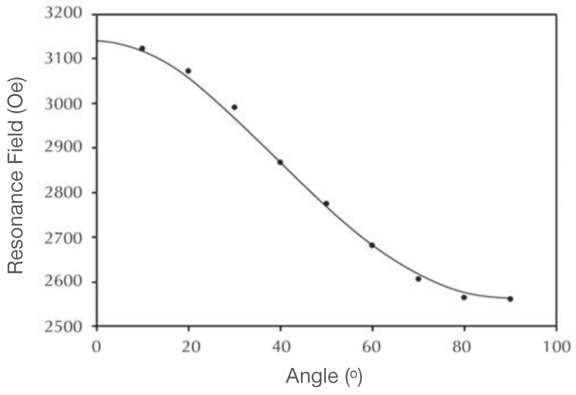
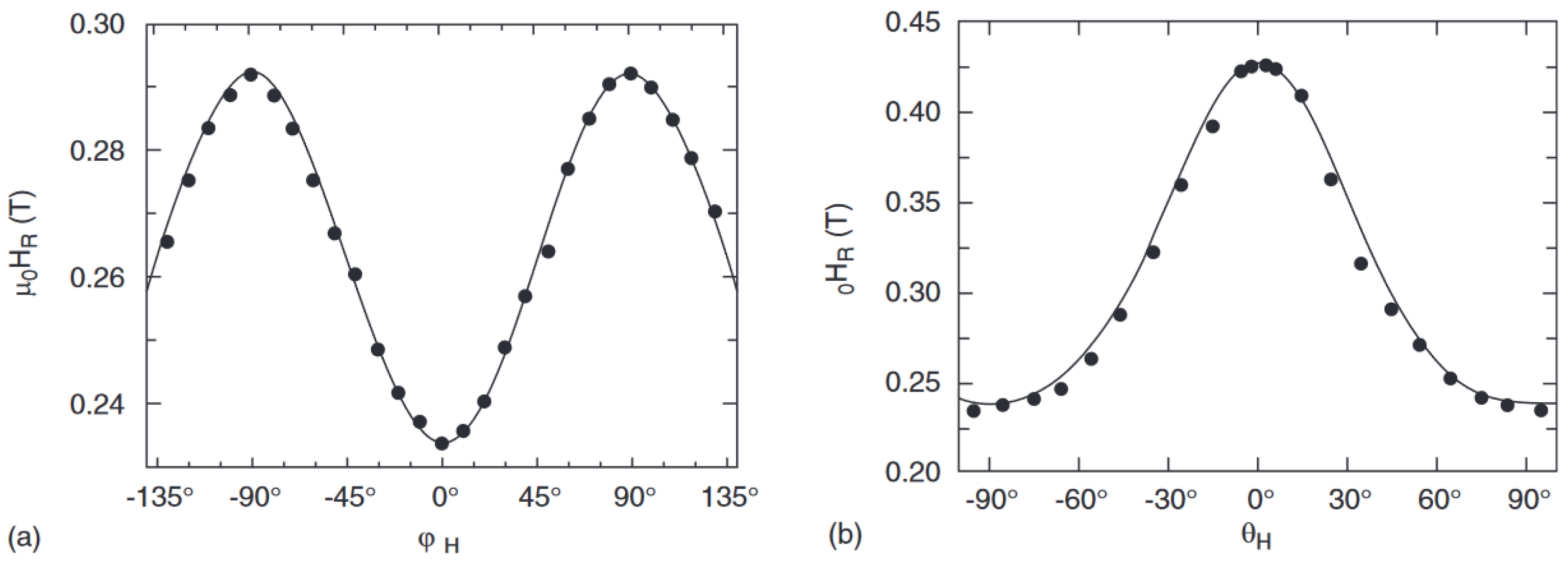
Self-assembly (regular arrays) of monodisperse Co FCC nanocrystals, with a diameter of 12 nm, were studied by Spasova et al. [88] using FMR. The effective magnetic resonance field was measured as a function of the orientation of the externally applied field with in-plane (azimuthal) and out-of-plane (polar) directions. For the interpretation of the angular dependencies of the resonance field ($H_r$), the authors considered the effective magnetic anisotropy of the individual particles (shape, volume, and surface contributions) and the shape anisotropy caused by the stripes and the magnetic anisotropy due to the particle interaction inside the stripe.

The in-plane resonance field could be obtained by introducing a cubic symmetry, in-plane uniaxial anisotropy, and the small in-plane shape anisotropy ($N_x,N_y\le \le N_z\approx 1$) as commonly used in thin films:

$$\begin{array}{cc}\hfill {\left(\frac{\omega }{\gamma }\right)}^2=& \left[H_{\mathrm{r}}+2H_{\mathrm{K}}^{4\parallel }cos4\phi -H_{\mathrm{K}}^{2\parallel }cos2\left(\phi -{\phi }_{\mathrm{u}}\right)\right]\hfill \\ \hfill & \times \left[H_{\mathrm{r}}+H_{\mathrm{eff}}+H_{\mathrm{K}}^{4\parallel I}\left(2-{sin}^{2}2\phi \right)\right.\left.-H_{\mathrm{K}}^{2\parallel }{cos}^2\left(\phi -{\phi }_{\mathrm{u}}\right)\right].\hfill \end{array}$$

(55)

where ${\phi }_{\mathrm{u}}$ is the angle of the applied external magnetic field with respect to the axis of in-plane uniaxial anisotropy. $H_{\mathrm{K}}^{2\parallel }$ and $H_{\mathrm{K}}^{4\parallel }$ are the effective uniaxial and four-fold in-plane magnetic anisotropy, respectively. The effective anisotropy field can be written as $H_{\mathrm{eff}}=\left(-2K_{2\perp }/M_{\mathrm{s}}\right)+4\pi \rho M_{\mathrm{s}}$, where $K_{2\perp }$ is the perpendicular anisotropy energy and $\rho$ the volumetric filling factor of the obtained stripes.

The fit of the experimental data using Equation (55) is shown (solid line) in Figure 26a and is in good agreement with the experiment. This fit gave $H_{\mathrm{K}}^{2\parallel }=0.037$ T, $H_{\mathrm{K}}^{4\parallel }=0$ (only uniaxial anisotropy is present) and $H_{\mathrm{eff}}=0.127$ T.

For the polar dependence of the applied magnetic field, the equation for the resonance gives:

$$\begin{array}{cc}\hfill {\left(\frac{\omega }{\gamma }\right)}^2=& \left[H_{\mathrm{r}}cos\left(\vartheta -\theta \right)-H_{\mathrm{eff}}cos2\vartheta \right]\hfill \\ \hfill & \times \left[H_{\mathrm{r}}cos\left(\vartheta -\theta \right)-H_{\mathrm{eff}}{cos}^2\vartheta +H_{\mathrm{K}}^{2\parallel }\right]\hfill \end{array}$$

(56)

the fit of the experimental data with the above equation (see Figure 26b) gives, once again, $H_{\mathrm{K}}^{2\parallel }=0.037$ T and $H_{\mathrm{eff}}=0.13$ T, without the requirement of incorporating fourth-order contributions. This particular uniaxial anisotropy is attributed to the shape anisotropy of the stripes and the potential alignment of the crystalline anisotropy axes of the individual crystals.

The FMR technique has also made it possible to study the effect of the dipole–dipole interaction in superparamagnetic nanoparticles. Slay et al. [23] have experimentally investigated iron-oxide (${\mathrm{Fe}}_3{\mathrm{O}}_4$) nanoparticles with an average diameter of (10 ± 1) nm. They developed a theoretical model that allowed them to fit the obtained FMR spectra in order to interpret these experimental results. For this, they considered contributions from the externally applied magnetic field, magnetocrystalline anisotropy, and shape anisotropy, which includes dipole–dipole interactions. The angle dependence of the resonance field at fixed frequency gives [23]:

$$\begin{array}{cc}\hfill {\left(\frac{\omega }{\gamma }\right)}^2=& {\mu }_0\{H[cos\vartheta cos\theta +cos(\varphi -\phi )sin\vartheta sin\theta ]\hfill \\ \hfill & +\left(H_{\mathrm{uni}}+2H_{\mathrm{cub}}\right)cos2\theta \hfill \\ \hfill & \left.-\frac{1}{2}{H}_{\mathrm{cub}}(7+cos4\varphi )(1+2cos2\theta )sin{\theta }^2\right\}\hfill \\ \hfill & \times \left\{H\right[cos\vartheta cos\theta +cos(\varphi -\phi )sin\vartheta sin\theta ]\hfill \\ \hfill & +\left(H_{\mathrm{uni}}+2H_{\mathrm{cub}}\right)cos{\theta }^2\hfill \\ \hfill & \left.-\frac{1}{2}{H}_{\mathrm{cub}}\left[4cos4\varphi -cos{\theta }^2(7+cos4\varphi )\right]sin{\theta }^2\right\}\hfill \end{array}$$

(57)

where $H_{\mathrm{cub}}=K_1/M_{\mathrm{s}}$ is the cubic magnetocrystalline anisotropy field and $H_{\mathrm{uni}}=N_{\mathrm{eff}}{M}_{\mathrm{s}}$ is the effective field due to dipolar interaction, with $N_{\mathrm{eff}}=N_{\perp }-N_{\Vert }$ is the effective demagnetizing tensor. Indeed, as it is not possible to explicitly calculate the dipole–dipole interactions for a group of particles, the authors represented the particle interactions as an effective anisotropy field called $H_{\mathrm{uni}}$.

The resonance field $H_{\mathrm{r}}(\vartheta ,\phi )$ was then computed from Equation (57) to produce individual FMR spectra for all $\vartheta$ and $\phi$ directions. This procedure was then repeated for a distribution of the particle sizes. The shape of each FMR spectrum can be described as a Gaussian derivative, which corresponds to the derivative of the imaginary part of the susceptibility ${\chi }^{″}$:

$$\frac{d{\chi }^{″}}{dH}=\sum _d{a}_d\sum _{\vartheta ,\phi }p\left(\vartheta \right)\frac{2\left[H-H_{\mathrm{r}}(\vartheta ,\phi )\right]}{\mathsf{\Delta }{H}_d^3\sqrt{2\pi }}{e}^{-{\left[\frac{H-H_{\mathrm{r}}\left({\theta }_{,}\phi \right)}{\mathsf{\Delta }{H}_d}\right]}^2}$$

(58)

In this context, the weight function $p\left(\vartheta \right)=sin\vartheta /4\pi$ is used to project the contribution of each resonance onto the field axis. It is assumed that the particle axes are uniformly distributed in orientation. Additionally, $\mathsf{\Delta }{H}_{\mathrm{d}}$ represents the linewidth distribution, and the parameter $a_{\mathrm{d}}$ scales the contribution of each particle size, which is assumed to follow a normal distribution:

$$a_d=\frac{1}{\sigma \sqrt{2\pi }}{e}^{\frac{1}{2}{\left(\frac{d-d_0}{\sigma }\right)}^2}$$

(59)

where $d_0$ = 10 nm is the average particle diameter, and $\sigma$ represents the particle size distribution, i.e., the deviation from $d_0$. More details on the theoretical model and the expression of the linewidth distribution are available on [23].

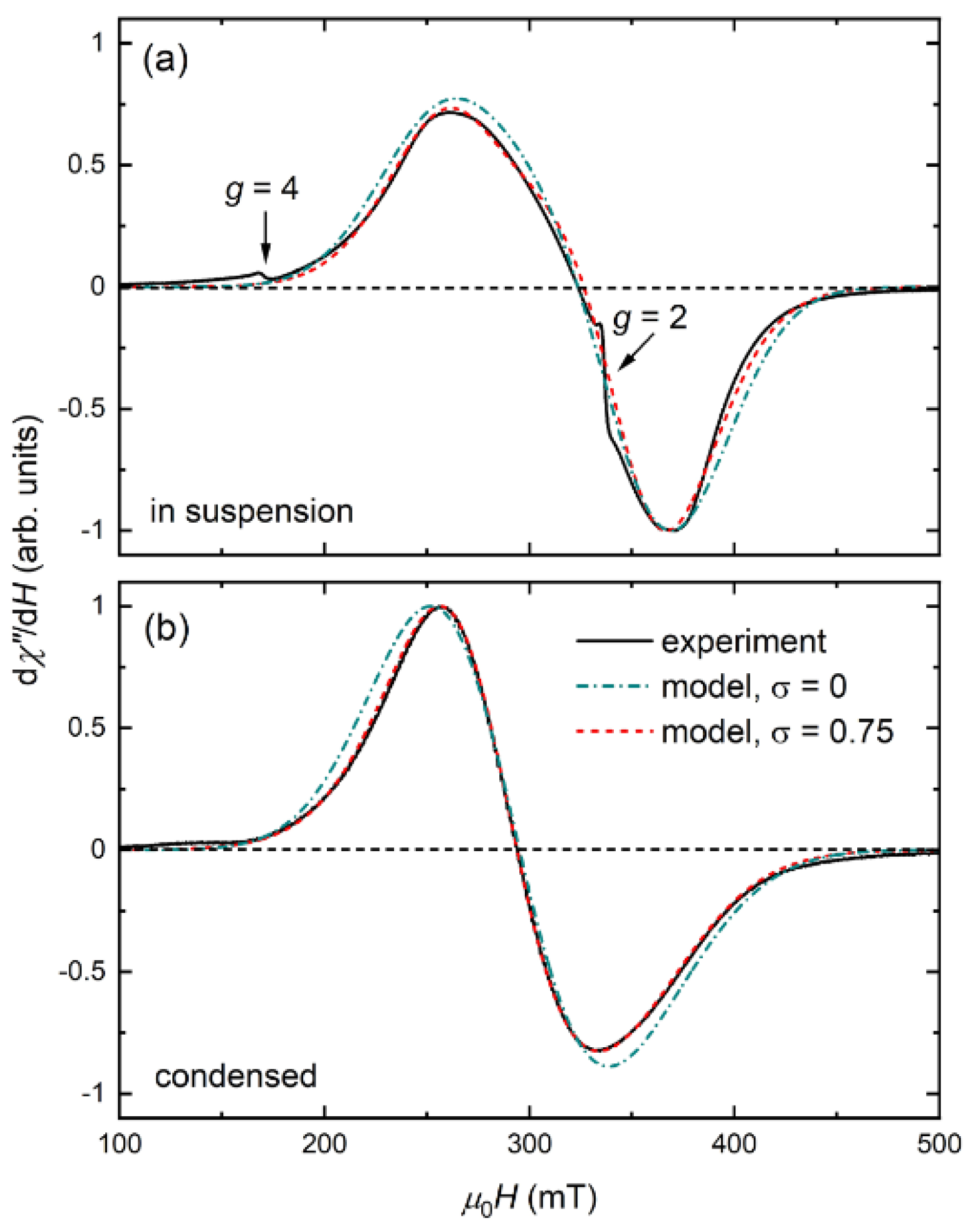
FMR measurements of suspended (in toluene) and dried commercial ${\mathrm{Fe}}_3{\mathrm{O}}_4$ nanoparticles have been carried out as shown in Figure 27. A difference is clearly visible between the FMR spectra for the particles in suspension and after drying. In suspension, the spectrum is asymmetric with a resonance field of ${\mu }_0{H}_{\mathrm{r}}$ = 323 mT. Additionally, sharp paramagnetic resonances are observed at 170 and 338 mT corresponding to g ≈ 4 and 2, respectively, in addition to the broad ferromagnetic spectrum. However, these features disappear upon drying, and the spectrum becomes symmetric with a resonance field of = ${\mu }_0{H}_{\mathrm{r}}$ 294 mT. Slay et al. [23] deducted that these sharp features are due to surface effects caused by surfactants (specifically, oleic acid) because they disappear once the surfactants are neutralized. Thus, the peak with g ≈ 4 was attributed to ${\mathrm{Fe}}^{3+}$ in a rhombohedrally distorted ligand field, and the peak with g ≈ 2 to ${\mathrm{OH}}^{-}$ radicals, as has already been demonstrated for a similar sample [89].

The fits with the developed model, yielded to ${\mu }_0{H}_{\mathrm{uni}}$ = 63 mT and ${\mu }_0{H}_{\mathrm{cub}}$ = −3 mT (using g = 2.11) for the nanoparticles in suspension, and ${\mu }_0{H}_{\mathrm{uni}}$ = −50 mT and ${\mu }_0{H}_{\mathrm{cub}}$ = −4 mT (using g = 2.24) for dried nanoparticles. Note that in comparing the two fits, with or without the distribution ($\sigma$), the parameters (g, $H_{\mathrm{uni}}$, $H_{\mathrm{cub}}$ and $\mathsf{\Delta }H$ ) varies only about $2\%$ between these two situations. Therefore, it is possible to fit these spectra with or without taking the distribution into consideration. However, by taking the distribution into account, the fit was significantly improved with high fidelity.

The ${\mu }_0{H}_{\mathrm{uni}}$ = 63 mT for the suspension, indicated an easy-axis symmetry with $N_{\mathrm{eff}}$ = 0.11, which corresponds to an average elongation of c/a ≈ 1.3 for the prolate ellipsoid. Despite the uniformly shaped particles with nearly spherical symmetry as observed in the TEM images [23], the value of $H_{\mathrm{uni}}$ is not a result of particle shape, but rather dipolar interactions between the particles. This assumption is supported by the change of sign of the dipolar field upon drying (from positive to negative), as it is the configuration of the nanoparticles that changes and not their shape. Indeed, in the dried state, when the nanoparticles cluster together, the anisotropy changes to easy-plane (negative uniaxial field). Thus, this modification in the magnetic properties illustrates the impact of dipole–dipole interactions in short timeframes since it is measurable within the FMR experiments with a ${10}^{-10}$ s time window.

6. Conclusions

Ferromagnetic resonance remains a powerful technique to investigate the magnetic properties of magnetic oxide nanoparticle assemblies. It has been demonstrated through several studies shown in this review that FMR is very useful to study the effect of temperature or doping on the magnetic properties of these nanoparticles. A variation in the FMR linewidth as a function of temperature or doping was observed. Therefore, we can conclude that magnetic damping (and its intrinsic or extrinsic contributions) is highly sensitive to the variation of these parameters. FMR has also made it possible to demonstrate the effect of the synthesis method on the magnetocrystalline anisotropy for the same nanoparticle.

References

1. Schmool, D.S. Ferromagnetic Resonance in Nanometric Magnetic Systems; Elsevier: Amsterdam, The Netherlands, 2016; p. 19. [Google Scholar]
2. Gazeau, F.; Bacri, J.; Gendron, F.; Perzynski, R.; Raikher, Y.; Stepanov, V.; Dubois, E. Magnetic resonance of ferrite nanoparticles: Evidence of surface effects. J. Magn. Magn. Mater. 1998, 186, 175–187. [Google Scholar] [CrossRef]
3. Arbab, A.; Tufail, S.; Rehmat, U.; Pingfan, Z.; Manlin, G.; Muhammad, O.; Zhiqiang, T.; YuKui, R. Review on Recent Progress in Magnetic Nanoparticles: Synthesis, Characterization, and Diverse Applications. Front. Chem. 2021, 9, 629054. [Google Scholar]
4. kianfar, E. Magnetic Nanoparticles in Targeted Drug Delivery: A Review. J. Supercond. Nov. Magn. 2021, 34, 1709–1735. [Google Scholar] [CrossRef]
5. Mitchell, E.; Gupta, R.K.; Mensah-Darkwa, K.; Kumar, D.; Ramasamy, K.; Gupta, B.K.; Kahol, P. Facile synthesis and morphogenesis of superparamagnetic iron oxide nanoparticles for high-performance supercapacitor applications. N. J. Chem. 2014, 38, 4344. [Google Scholar] [CrossRef]
6. Chhaganlal, G.A.; Pradeep, R.; Yu-Chen, Y.; Tai-Yue, L.; Chi-Yuan, W.; Hayakawa, Y.; Yun, W.S. Understanding the Magnetic Memory Effect in Fe-Doped NiO Nanoparticles for the Development of Spintronic Devices. ACS Appl. Nano Mater. 2019, 2, 278–290. [Google Scholar]
7. Hirohata, A.; Takanashi, K. Future perspectives for spintronic devices. J. Phys. D Appl. Phys. 2014, 47, 193001. [Google Scholar] [CrossRef]
8. Puebla, J.; Kim, J.; Kondou, K.; Yoshichika, O. Spintronic devices for energy-efficient data storage and energy harvesting. Commun. Mater. 2020, 1, 24. [Google Scholar] [CrossRef]
9. Barla, P.; Joshi, V.K.; Bhat, S. Spintronic devices: A promising alternative to CMOS devices. J. Comput. Electron. 2021, 20, 805–837. [Google Scholar] [CrossRef]
10. Barman, A.; Haldar, A. Time-Domain Study of Magnetization Dynamics in Magnetic Thin Films and Micro- and Nanostructures. Solid State Phys. 2014, 65, 1–108. [Google Scholar]
11. Sima, M.; Fatemeh, Z.S.; Mussa, F.S.; Mehdi, S.G.; Abolfazl, A. Current methods for synthesis of magnetic nanoparticles. Artif. Cells Nanomed. Biotechnol. 2016, 44, 722–734. [Google Scholar]
12. Jing, X.; Haibin, Y.; Wuyou, F.; Kai, D.; Yongming, S.; Jiuju, C.; Yi, Z.; Minghui, L.; Guangtian, Z. Preparation and magnetic properties of magnetite nanoparticles by sol–gel method. J. Magn. Magn. Mater. 2007, 309, 307–311. [Google Scholar]
13. Atiqur, R.M.; Tariqul, I.M.; Jit, S.M.S.; Samsuzzaman, M.; Samsuzzaman, M.E.H. Synthesis and characterization of Mg–Zn ferrite based flexible microwave composites and its application as SNG metamaterial. Sci. Rep. 2021, 11, 7654. [Google Scholar]
14. Pessoa, M.; Moscon, P.; Melo, R.; Franco, A.; Morais, P. A comprehensive study of Co1-xNixFe2O4 nanoparticles fabricated via three different synthetic methods. Mater. Res. Express 2019, 6, 125068. [Google Scholar] [CrossRef]
15. Prashant, K.; Khanduri, H.; Saurabh, P.; Arjun, S.; Basheed, G.A.; Pant, R.P. Temperature selectivity for single phase hydrothermal synthesis of PEG-400 coated magnetite nanoparticles. Dalton Trans. 2020, 49, 8672–8683. [Google Scholar]
16. Arkadýev, V.K. The Reflection of Electric Waves from a Wire. Sov. Phys.-JETP 1913, 45A, 45312. [Google Scholar]
17. Landau, L. Über die Elektrodynamik der Kristallgitter. Phys. Z. Der Sowjetunion 1935, 8, 165. [Google Scholar]
18. Vonsovskii, V. Ferromagnetic Resonance; Pergamon Press: Oxford, UK, 1966. [Google Scholar]
19. Smit, J.; Beljers, H.G. Ferromagnetic Hysteresis in Single Crystals of Hematite (Fe2O3). Philips Res. Rep. 1955, 10, 113–130. [Google Scholar]
20. Farle, M. Magnetic nanoparticles: Synthesis, protection, functionalization, and application. Rep. Prog. Phys. 1998, 61, 755–788. [Google Scholar] [CrossRef]
21. Osborn, J.A. Demagnetizing Factors of the General Ellipsoid. Phys. Rev. 1945, 67, 351. [Google Scholar] [CrossRef]
22. MacDonald, J.R. Ferromagnetic Resonance and the Internal Field in Ferromagnetic Materials. Proc. Phys. Soc. A 1951, 64, 968. [Google Scholar] [CrossRef]
23. Slay, D.; Cao, D.; Ferré, E.C.; Charilaou, M. Ferromagnetic resonance of superparamagnetic nanoparticles: The effect of dipole–dipole interactions. J. Appl. Phys. 2021, 130, 113902. [Google Scholar] [CrossRef]
24. Skomski, R.; Hadjipanayis, G.C.; Sellmyer, D.J. Effective Demagnetizing Factors of Complicated Particle Mixtures. IEEE Trans. Magn. 2007, 43, 6. [Google Scholar] [CrossRef] [Green Version]
25. Schmool, D.S. Nanotechnologies: The Physics of Nanomaterials. In The Physics of Surfaces and Nanofabrication Techniques; Apple Academic Press (CRC Press, Taylor and Francis Group): Cambridge, MA, USA, 2021; Volume 1. [Google Scholar]
26. Kachkachi, H.; Dimian, M. Hysteretic properties of a magnetic particle with strong surface anisotropy. Phys. Rev. B 2002, 66, 174419. [Google Scholar] [CrossRef] [Green Version]
27. Kachkachi, M.; Bonet, E. Surface-induced cubic anisotropy in nanomagnets. Phys. Rev. B 2006, 73, 224402. [Google Scholar] [CrossRef] [Green Version]
28. Jamet, M.; Wernsdorfer, W.; Thirion, C.; Dupuis, V.; Mélinon, P.; Pérez, A.; Mailly, D. Magnetic anisotropy in single clusters. Phys. Rev. B 2004, 69, 024401. [Google Scholar] [CrossRef]
29. Bodker, F.; Mørup, S.; Linderoth, S. Surface effects in metallic iron nanoparticles. Phys. Rev. Lett. 1994, 72, 282. [Google Scholar] [CrossRef] [Green Version]
30. Herzer, G.M. (Ed.) Properties and Applications of Nanocrystalline Alloys from Amorphous Precursors; NATO ARW Series; Kluwer: Alphen aan den Rijn, The Netherlands, 2005; p. 15234. [Google Scholar]
31. Herzer, G. Nanocrystalline Soft Magnetic Alloys. In Handbook of Magnetic Material; Buchow, K.H.J., Ed.; 1997; Volume 10, pp. 415–462. [Google Scholar]
32. Alben, R.; Becker, J.J.; Chi, M.C. Random anisotropy in amorphous ferromagnets. JAP 1978, 49, 1653–1658. [Google Scholar] [CrossRef]
33. Chudnovsky, E.M.; Saslow, W.M.; Serota, R.A. Ordering in ferromagnets with random anisotropy. Phys. Rev. B 1986, 33, 251. [Google Scholar] [CrossRef]
34. Suzuki, K.; Herzer, G. Soft Magnetic Nanostructures and Applications. In Advanced Magnetic Nanostructures; Springer: Lincoln, NE, USA, 2006. [Google Scholar]
35. Cacciola, G.; Berdie, J. Surface effects on the wetting properties of nanofluids. Acta Phys. Pol. A 2016, 129, 88–91. [Google Scholar] [CrossRef]
36. Schmool, D.S.; Schmalzl, K. Ferromagnetic resonance in magnetic nanoparticle assemblies. J. Non-Cryst. Solids 2007, 353, 738–742. [Google Scholar] [CrossRef]
37. Schmool, D.S.; Schmalzl, K. Magnetic dipolar interaction in nanoparticle systems: Theory, simulation and ferromagnetic resonance. In Advances in Nanoscale Magnetism; Springer: Berlin/Heidelberg, Germany, 2009; pp. 321–326. [Google Scholar]
38. Schmool, D.S.; Rocha, R.; Sousa, J.B.; Santos, J.A.M.; Kakazei, G.N.; Garitaonandia, J.S.; Lezama, L. The role of dipolar interactions in magnetic nanoparticles: Ferromagnetic resonance in discontinuous magnetic multilayers. J. Appl. Phys. 2007, 101, 103907. [Google Scholar] [CrossRef]
39. Netzelmann, U. Magnetic susceptibility of YBa2Cu3O7 single crystals. JAP 1990, 68, 1800–1806. [Google Scholar]
40. Dubowik, J.; Rakowski, M.; Baran, M. Anisotropic magnetic susceptibility of TmSe. Phys. Rev. B 1996, 54, 1088–1092. [Google Scholar] [CrossRef]
41. Kakazei, G.N.; Pleshchev, V.G.; Poltavtsev, S.V. Magnetic properties of quasicrystals AlNiCo and AlCuFe. JAP 1999, 85, 5654–5657. [Google Scholar]
42. Morup, S.; Christensen, M.; Bechgaard, K. Magnetic nanoparticles: Synthesis, stabilization, functionalization, characterization, and applications. Beilstein J. Nanotechnol. 2010, 1, 182–210. [Google Scholar]
43. Néel, L. Théorie du trainage magnétique des ferromagnétiques en grains fins avec applications aux terres cuites. Années de Géophysique 1949, 5, 99–136. [Google Scholar]
44. Brown, W.F. Thermal fluctuations of a single-domain particle. Phys. Rev. 1963, 130, 1677. [Google Scholar] [CrossRef]
45. Chantrell, R. W; Wohlfarths, E.P. Rate Dependence of the Field-Cooled Magnetisation of a Fine Particle System. Phys. Status Solidi 1985, 91, 619–626. [Google Scholar] [CrossRef]
46. Stoner, E.C.; Wohlfarth, E.P. A Mechanism of Magnetic Hysteresis in Heterogeneous Alloys. Philos. Trans. R. Soc. A Math. Phys. Eng. Sci. 1948, 240, 599–642. [Google Scholar] [CrossRef]
47. Tannous, C.; Gieraltowski, J. The Stoner–Wohlfarth model of ferromagnetism. Eur. J. Phys. 2008, 29, 475. [Google Scholar] [CrossRef]
48. Guardia, P.; Batlle-Brugal, B.; Roca, A.G.; Iglesias, O.; Morales, M.P.; Serna, C.J.; Labarta, A.; Batlle, X. Surfactant effects in magnetite nanoparticles of controlled size. J. Magn. Magn. Mater. 2007, 316, e756–e759. [Google Scholar] [CrossRef] [Green Version]
49. Antoniak, C.; Lindner, J.; Farle, M. Magnetic anisotropy and its temperature dependence in iron-rich FexPt1-x nanoparticles. Europhys. Lett. 2005, 70, 250. [Google Scholar] [CrossRef]
50. Dormann, J.L.; Bessais, L.; Fiorani, D. A dynamic study of small interacting particles: Superparamagnetic model and spin-glass laws. J. Phys. C Solid State Phys. 1988, 21, 2015. [Google Scholar] [CrossRef]
51. Shtrikman, S.; Wohlfarth, E. The theory of the Vogel-Fulcher law of spin glasses. Phys. Lett. A 1981, 85, 467–470. [Google Scholar] [CrossRef]
52. Djurberg, C.; Svedlindh, P.; Nordblad, P.; Hansen, M.F.; Bødker, F.; Mørup, S. Dynamics of an Interacting Particle System: Evidence of Critical Slowing Down. Phys. Rev. Lett. 1997, 79, 5154–5157. [Google Scholar] [CrossRef] [Green Version]
53. Toulemon, D.; Mircea, V.R.; Schmool, D.; Garitaonandia, J.S.; Lezama, L.; Cattoen, X.; Begin-Colin, S.; Pichon, B.P. Iron Oxide Nanoparticles: Enhanced Collective Magnetic Properties Induced by the Controlled Assembly of Iron Oxide Nanoparticles in Chains. Adv. Funct. Mater. 2016, 26, 2583. [Google Scholar] [CrossRef]
54. Charilaou, M. Ferromagnetic resonance of biogenic nanoparticle-chains. JAP 2017, 122, 063903. [Google Scholar] [CrossRef]
55. Steen, M.; Elisabeth, T. Superparamagnetic relaxation of weakly interacting particles. Phys. Rev. Lett. 1994, 72, 3278–3281. [Google Scholar]
56. Pereira, A.M.; Pereira, C.; Silva, A.S.; Schmool, D.S.; Freire, C.; Greneche, J.M.; Araujo, J.P. Unravelling the effect of interparticle interactions and surface spin canting in γ-Fe2O3SiO2 superparamagnetic nanoparticles. JAP 2011, 109, 114319. [Google Scholar]
57. de Biasi, R.S.; Devezas, T.C. Anisotropy field of small magnetic particles as measured by resonance. JAP 1978, 49, 2466–2469. [Google Scholar] [CrossRef]
58. Berger, R.; Kliava, J.; Bissey, J.C.; Baietto, V. Superparamagnetic resonance of annealed iron-containing borate glass. J. Phys. Condens. Matter 1998, 10, 8559. [Google Scholar] [CrossRef]
59. Berger, R.; Kliava, J. Size and shape distribution of magnetic nanoparticles in disordered systems: Computer simulations of superparamagnetic resonance spectra. J. Magn. Magn. Mater. 1999, 205, 328–342. [Google Scholar]
60. Heinrich, B. Spin relaxation in magnetic metallic layers and multilayers. In Ultrathin Magnetic Structures III: Fundamentals of Nanomagnetism; Bland, J.A.C., Heinrich, B., Eds.; Springer: Berlin/Heidelberg, Germany, 2005; p. 143. [Google Scholar]
61. Vittoria, C.; Barker, R.C.; Yelon, A. Anisotropic Ferromagnetic Resonance Linewidth in Ni Platelets. Phys. Rev. Lett. 1967, 19, 792. [Google Scholar] [CrossRef]
62. Evgeny, G.; Miroslav, S.; Mingxi, W.; Liudmila, A.; Dmitrii, M.; Ekaterina, K.; Vasilii, L.; Evgeny, A.; Boris, G.; Oleg, B.; et al. Tuning the particle size, natural ferromagnetic resonance frequency and magnetic properties of -Fe 2 O 3 nanoparticles prepared by a rapid sol–gel method. J. Mater. Chem. C 2021, 9, 6173–6179. [Google Scholar]
63. Jin, J.; Ohkoshi, S.I.; Hashimoto, K. Giant Coercive Field of Nanometer Sized Iron Oxide. Adv. Mater. 2004, 12, 48–51. [Google Scholar] [CrossRef]
64. Pessoa, M.; Proveti, J.; Pelegrini, F.; Moscon, P. Ferromagnetic resonance lines of annealed Ni ferrites. Phys. B Condens. Matter 2019, 558, 20–23. [Google Scholar] [CrossRef]
65. Tsay, F.D.; Chan, S.; Manatt, S.L. Ferromagnetic resonance of lunar samples. Geochim. Cosmochim. Acta 1971, 35, 865–875. [Google Scholar] [CrossRef]
66. Mantilla, J.; Felix, L.L.; Rodriguez, M.; Aragon1, F.; Morais, P.; Coaquira, J.; Kuzmann, E.; de Oliveira, A.; Gonzalez, I.; Macedo, W.; et al. Washing effect on the structural and magnetic properties of NiFe2O4 nanoparticles synthesized by chemical sol-gel method. Mater. Chem. Phys. 2018, 211, 1–17. [Google Scholar]
67. Gandhi, A.C.; Lin, J.C. Magnetic resonance study of exchange-biased Ni/NiO nanoparticles. J. Phys. Condens. Matter 2017, 29, 215802. [Google Scholar] [CrossRef] [PubMed]
68. Gandhi, A.C.; Lin, J.C. Exchange bias in finite sized NiO nanoparticles with Ni clusters. J. Magn. Magn. Mater. 2017, 424, 221–225. [Google Scholar] [CrossRef]
69. Raikher, Y.L.; Stepanov, V.I. The effect of thermal fluctuations on the FMR line shape in dispersed ferromagnets. Sov. Phys. JETP 1992, 75, 764. [Google Scholar]
70. Hernández-Gómez, P.; Valente, M.A.; Graça, M.P.F.; Muñoz, J.M. Synthesis, structural characterization and broadband ferromagnetic resonance in Li ferrite nanoparticles. J. Alloys Compd. 2018, 765, 186–192. [Google Scholar] [CrossRef] [Green Version]
71. Azzawi, S.; Hindmarch, A.T.; Atkinson, D. Magnetic damping phenomena in ferromagnetic thin-films and multilayers. J. Phys. D Appl. Phys. 2017, 50, 473001. [Google Scholar] [CrossRef]
72. Castel, V.; Youssef, J.B.; Brosseau, C. Broadband ferromagnetic resonance measurements in Ni/ZnO and Niy-Fe2O3 nanocomposites. J. Nanomater. 2007, 27437, 16. [Google Scholar]
73. Hernandez-Gomez, P.; Munoz, J.; Valente, M. Field-induced microwave absorption in Ni ferrite nanoparticles. IEEE Trans. Magn. 2010, 46, 475–478. [Google Scholar] [CrossRef]
74. Yang, H.; Wang, Z.; Song, L.; Zhao, M.; Wang, J.; Luo, H. A study on the coercivity and the magnetic anisotropy of the lithium ferrite nanocrystallite. J. Phys. D Appl. Phys. 1996, 29, 2574. [Google Scholar] [CrossRef]
75. Hernandez Gomez, P.; Munoz, J.M.; Valente, M.A.; Graça, M.P.F. Broadband ferromagnetic resonance in Mn doped Li ferrite nanoparticles. Mater. Res. Bull. 2019, 112, 432–437. [Google Scholar] [CrossRef]
76. White, O.; Patton, C. Magnetic properties of lithium ferrite microwave materials. J. Magn. Magn. Mater. 1978, 9, 299–317. [Google Scholar] [CrossRef]
77. Argentina, B.G.; Courtney, W.; Dionne, G.; Temme, D. Lithium ferrites for microwave devices. IEEE Trans. Magn. 1972, 8, 83–94. [Google Scholar]
78. Datt, G.; Kotabageb, C.; Abhyankar, A.C. Ferromagnetic resonance of NiCoFe2O4 nanoparticles and microwave absorption properties of flexible NiCoFe2O4–carbon black/poly(vinyl alcohol) composites. Phys. Chem. Chem. Phys. 2017, 19, 20699–20712. [Google Scholar] [CrossRef]
79. Yanez-Vilar, S.; Sanchez-Andujar, M.; Gomez-Aguirre, C.; Mira, J.; Senaris-Rodriguez, M.; Castro-Garcia, S. A simple solvothermal synthesis of MFe2O4 (M=Mn, Co and Ni) nanoparticles. J. Solid State Chem. 2009, 182, 2685–2690. [Google Scholar] [CrossRef] [Green Version]
80. Dutta, P.; Manivannan, A.; Seehra, M.; Shah, N.; Huffman, G. Magnetic properties of nearly defect-free maghemite nanocrystals. Phys. Rev. B 2004, 70, 174428. [Google Scholar] [CrossRef]
81. Weil, J.A.; Bolton, J.R. Electron Paramagnetic Resonance Elementary Theory and Practical Applications, 2nd ed.; John Wiley & Sons, Inc.: Hoboken, NJ, USA, 2007. [Google Scholar]
82. Datt, G.; Bishwas, M.S.; Raja, M.M.; Abhyankar, A.C. Observation of magnetic anomalies in onestep solvothermally synthesized nickel–cobalt ferrite nanoparticles. Nanoscale 2016, 8, 5200–5213. [Google Scholar] [CrossRef] [PubMed]
83. Chien-Yie, T.; Yi-Chun, C.; Yung-Kuan, T. Investigation on structural, magnetic, and FMR properties for hydrothermally-synthesized magnesium-zinc ferrite nanoparticles. Phys. B Condens. Matter 2019, 570, 29–34. [Google Scholar]
84. Gama, L.; Hernandez, E.; Cornejo, D.; Costa, A.; Rezendea, S.; Kiminami, R.; Costa, A. Magnetic and structural properties of nanosize Ni–Zn–Crferrite particles synthesized by combustion reaction. J. Magn. Magn. Mater. 2007, 317, 29–33. [Google Scholar] [CrossRef]
85. Angadi, V.J.; Choudhury, L.; Sadhana, K.; Liu, H.L.; Sandhya, R.; Matteppanavar, S.; Rudraswamy, B.; Pattar, V.; Anavekar, R.V.; Praveena, K. Structural, electrical and magnetic properties of Sc3+ doped Mn-Zn ferrite nanoparticles. J. Magn. Magn. Mater. 2017, 424, 1–11. [Google Scholar] [CrossRef]
86. Sharma, V.; Kumari, S.; Kuanr, B.K. Rare earth doped M-type hexaferrites; ferromagnetic resonance and magnetization dynamics. AIP Adv. 2018, 8, 056232. [Google Scholar] [CrossRef] [Green Version]
87. Bastrukov, S.; Khoo, J.Y.; Lukiyanchuk, B.; Molodtsova, I. Micromagnetic theory of spin relaxation and ferromagnetic resonance in multilayered metallic films. arXiv 2012, arXiv:1210.2609. [Google Scholar]
88. Spasova, M.; Wiedwald, U.; Ramchal, R.; Farle, M.; Hilgendorff, M.; Giersig, M. Magnetic properties of arrays of interacting Co nanocrystals. J. Magn. Magn. Mater. 2002, 240, 40–43. [Google Scholar] [CrossRef]
89. Amstad, E.; Fischer, H.; Gehring, A.U.; Textor, M.; Reimhul, E. Magnetic Decoupling of Surface Fe3+ in Magnetite Nanoparticles upon Nitrocatechol-Anchored Dispersant Binding. Chem. Eur. J. 2011, 17, 7396–7398. [Google Scholar] [CrossRef]
Figure 1. Diagram showing different time scales characteristic of various types of magnetization dynamics. Reprinted with permission from A. Barman and A. Haldar, Time-Domain Study of Magnetization Dynamics in Magnetic Thin Films and Micro and Nanostructures, Solid State Physics, 65, 1-108. Copyright (2014) Elsevier.
Magnetochemistry 09 00191 g001
Figure 2. MgZnFe 2 O 4  nanoparticle preparation by sol-gel method. The figure shows the preparation steps and the transition from the “sol” to the “gel” state [13]. This figure was published in Rahman Md Atiqur, Islam Mohammad Tariqul, Singh Mandeep Singh Jit, Samsuzzaman Md and Chowdhury Muhammad E. H., Synthesis and characterization of Mg–Zn ferrite based flexible microwave composites and its application as SNG metamaterial, 11, Scientific Reports, 2021. Open access, Springer Nature. Creative Commons licence, https://creativecommons.org/licenses/by/4.0/, accessed on 10 July 2023.
Magnetochemistry 09 00191 g002
Figure 3. A schematic diagram illustrating the hydrothermal synthesis of PEG-400-coated  Fe 3 O 4  magnetic nanoparticles at various reaction temperatures by using  FeCl 3  and  FeCl 2  as precursor salts, and polyethylene glycol (PEG-400) as surfactant. Reprinted with permission from Kumar Prashant, Khanduri H., Pathak Saurabh, Singh Arjun, Basheed G. A. and Pant R. P., Temperature selectivity for single phase hydrothermal synthesis of PEG-400 coated magnetite nanoparticles, Dalton Transactions, 49, 8672. Copyright (2020) ROYAL SOCIETY OF CHEMISTRY.
Magnetochemistry 09 00191 g003
Figure 4. (a) Schematic representation of the random anisotropy model, where arrows indicate the randomly fluctuating anisotropy axes and the hatched area represents the ferromagnetic (FM) correlation volume, which is determined by the exchange length,  λ ex . (Based on the RA model of [31]. Figure adapted from G. Herzer, Nanocrystalline soft magnetic alloys. In: Buschow, K.H.J. (Ed.), Handbook of Magnetic Materials, vol. 10, Elsevier Science 1997, 4152462. (b) Random average anisotropies. Figure adapted with permission from K. Suzuki and G. Herzer, Soft magnetic nanostructures and applications. In: D. Sellmyer and R. Skomski (Eds.), Advanced Magnetic Nanostructures, Springer Nature (2006).
Magnetochemistry 09 00191 g004
Figure 5. Angular dependence of the resonance field for a sample of  γ -Fe 2 O 3  nanoparticles with mean particle diameters of 4.6 nm. The line is a fit to Equation (27). Reprinted with permission from D. S. Schmool and K. Schmalzl, Ferromagnetic resonance in magnetic nanoparticle assemblies, Journal of Non-Crystalline Solids, 353(8-10), 738. Copyright (2007) Elsevier.
Magnetochemistry 09 00191 g005
Figure 6. The effect of size distribution is illustrated where a distribution of blocking temperatures is predicted for FMR and SQUID magnetometry. The calculations use  τ S Q U I D 10 2  s, τ F M R 10 10  s, where the inset shows a transmission electron microscope (TEM) image of the FePt NPs, from which the size distribution is determined. Reprinted with permission from C. Antoniak and J. Lindner and M. Farle, Magnetic anisotropy and its temperature dependence in iron-rich  Fe x Pt 1 x  nanoparticles, Europhys. Lett., 70, 20. Copyright (2005) IOP Publishing.
Magnetochemistry 09 00191 g006
Figure 7. Experimental data points at the specific temperatures with a fit using the Langevin function (line) from Equation (38). Reprinted with permission from D. S. Schmool and K. Schmalzl, Ferromagnetic resonance in magnetic nanoparticle assemblies, Journal of Non-Crystalline Solids, 353(8-10), 738. Copyright (2007) Elsevier.
Magnetochemistry 09 00191 g007
Figure 8. The phase composition in weight % of  Fe 2 O 3  samples calculated by a full profile analysis of the XRD patterns.  γ Fe 2 O 3  (yellow),  ϵ Fe 2 O 3  (turquoise), and  α Fe 2 O 3  (orange). Reprinted with permission from Gorbachev Evgeny, Soshnikov Miroslav, Wu Mingxi, et al., Tuning the particle size, natural ferromagnetic resonance frequency and magnetic properties of  Fe 2 O 3  nanoparticles prepared by a rapid sol–gel method, Journal of Materials Chemistry C, 9, 6173. Copyright (2021) ROYAL SOCIETY OF CHEMISTRY.
Magnetochemistry 09 00191 g008
Figure 9. Damping factor  γ  of the natural ferromagnetic resonance for  Fe 2 O 3  nanoparticles. Reprinted with permission from Gorbachev Evgeny, Soshnikov Miroslav, Wu Mingxi, et al., Tuning the particle size, natural ferromagnetic resonance frequency and magnetic properties of  Fe 2 O 3  nanoparticles prepared by a rapid sol–gel method, Journal of Materials Chemistry C, 9, 6173. Copyright (2021) ROYAL SOCIETY OF CHEMISTRY.
Magnetochemistry 09 00191 g009
Figure 10. X-ray diffraction of nanostructured Ni ferrite powders, annealed at 600 °C, 900 °C, and 1100 °C. Reprinted with permission from M.S. Pessoa, J.R.C. Proveti, F. Pelegrini and P.S. Moscon, Ferromagnetic resonance lines of annealed Ni ferrites, Physica B: Condensed Matter, 558, 20–23. Copyright (2019) Elsevier.
Magnetochemistry 09 00191 g010
Figure 11. FMR spectrum of Ni ferrites samples isothermally treated at (a) 600 °C, (b) 900 °C, and (c) 1100 °C obtained at room temperature at a microwave frequency of 9.8 Ghz. Solid lines represent experimental results and dashed lines are fitting using the equation in [64,65]. Reprinted with permission from M.S. Pessoa, J.R.C. Proveti, F. Pelegrini and P.S. Moscon, Ferromagnetic resonance lines of annealed Ni ferrites, Physica B: Condensed Matter, 558, 20–23. Copyright (2019) Elsevier.
Magnetochemistry 09 00191 g011
Figure 12. Results of XRD spectra for Ni samples annealed with  t A  from 10 to 600 min. (Upper panel) the obtained grain size and (lower panel) the values of lattice constants of Ni and NiO as a function of  t A  [67]. Reprinted with permission from Gandhi Ashish Chhaganlal and Lin Jauyn Grace, Magnetic resonance study of exchange-biased Ni/NiO nanoparticles, Journal of Physics: Condensed Matter, 29, 215802. Copyright (2017) IOP Publishing.
Magnetochemistry 09 00191 g012
Figure 13. (a) Room temperature FMR spectra for different annealing times. (b) Three lines were obtained after deconvolution of the FMR line for the sample at 600 min. (c) The effective g-factor and (d) Linewidth for these three peaks as a function of  t A . Reprinted with permission from Gandhi Ashish Chhaganlal and Lin Jauyn Grace, Magnetic resonance study of exchange-biased Ni/NiO nanoparticles, Journal of Physics: Condensed Matter, 29, 215802. Copyright (2017) IOP Publishing.
Magnetochemistry 09 00191 g013
Figure 14. The temperature effects of (a g e f f 1 , (b g e f f 2 , (c Δ H 1  and (d Δ H 2  for different annealing times. Three regions are separated by dotted vertical lines: I (330 K–200 K), II (200 K–130 K), and III (130 K–90 K). Inset of (d Δ H 2  versus (1/T) is plotted. Reprinted with permission from Gandhi Ashish Chhaganlal and Lin Jauyn Grace, Magnetic resonance study of exchange-biased Ni/NiO nanoparticles, Journal of Physics: Condensed Matter, 29, 215802. Copyright (2017) IOP Publishing.
Magnetochemistry 09 00191 g014
Figure 15. FMR resonance line of  α LiFe 5 O 8  nanoparticles annealed at 400 °C at different frequencies. Reprinted with permission from P. Hernandez-Gomez, M.A. Valente, M.P.F. Graça and J.M. Munoz, Synthesis, structural characterization and broadband ferromagnetic resonance in Li ferrite nanoparticles, Journal of Alloys and Compounds, 765, 186. Copyright (2018) Elsevier.
Magnetochemistry 09 00191 g015
Figure 16. On the left: linewidth of ferromagnetic resonance versus frequency for the Li ferrite nanoparticles annealed at 400 °C. On the right: resonance frequency versus magnetic resonance field for Li ferrite nanoparticles annealed from 400 to 1000 °C. Reprinted with permission from P. Hernandez-Gomez, M.A. Valente, M.P.F. Graça and J.M. Munoz, Synthesis, structural characterization and broadband ferromagnetic resonance in Li ferrite nanoparticles, Journal of Alloys and Compounds, 765, 186. Copyright (2018) Elsevier.
Magnetochemistry 09 00191 g016
Figure 17. Resonance frequency versus magnetic resonance field for Mn-doped Li ferrite nanoparticles annealed from 400 to 1000 °C in relation to bulk ferrite. Reprinted with permission from P. Hernandez-Gomez, J.M. Munoz, M.A. Valente and M.P.F. Graça, Broadband ferromagnetic resonance in Mn-doped Li ferrite nanoparticles, Materials Research Bulletin, 112, 432. Copyright (2019) Elsevier.
Magnetochemistry 09 00191 g017
Figure 18. FMR spectra of (a) ap-NCF and (b) an-NCF nanoparticles at temperature range from 100 K to 300 K. The inset: representative Gaussian fitting for ap-NCF sample at 300 K. Reprinted with permission from G. Datt, C. Kotabageb and A. C. Abhyankar, Ferromagnetic resonance of NiCoFe2O4 nanoparticles and microwave absorption properties of flexible NiCoFe2O4—carbon black/poly(vinyl alcohol) composites, Phys. Chem. Chem. Phys., 19, 20699. Copyright (2017) ROYAL SOCIETY OF CHEMISTRY.
Magnetochemistry 09 00191 g018
Figure 19. FMR spectra for (a γ Fe 2 O 3  nanoparticles at various temperatures with 9.28 Ghz on frequency, (b γ Fe 2 O 3  bulk, nanoparticles, and suspended nanoparticles at 300 K. Reprinted with permission from P. Dutta, A. Manivannan, M.S. Seehra, N. Shah and G.P. Huffman, Magnetic properties of nearly defect-free maghemite nanocrystals, Phys. Rev. B, 70. Copyright (2004) American Physical Society.
Magnetochemistry 09 00191 g019
Figure 20. Distribution of blocking temperatures for  τ F M R 10 10  s and  τ S Q U I D 10 2  s. The size distribution is determined from a transmission electron microscope (TEM) image of the FePt NPs, as shown in Figure 6. Reprinted with permission from C. Antoniak and J. Lindner and M. Farle, Magnetic anisotropy and its temperature dependence in iron-rich  Fe x Pt 1 x  nanoparticles, Europhys. Lett., 70, 20. Copyright (2005) IOP Publishing.
Magnetochemistry 09 00191 g020
Figure 21. (Left): particle size distribution of Zn-doped Mg ferrites nanoparticles extracted from TEM images. (Right): FMR spectra at 9.8 GHz frequency for  Mg 1 x Zn x Fe 2 O 4  nanoparticles. Reprinted with permission from Tsay Chien-Yie, Chiu Yi-Chun and Tseng Yung-Kuan, Investigation on structural, magnetic, and FMR properties for hydrothermally-synthesized magnesium-zinc ferrite nanoparticles, Physica B: Condensed Matter, 570, 29. Copyright (2019) Elsevier.
Magnetochemistry 09 00191 g021
Figure 22. FMR spectra of  Mg 1 x Zn x Fe 2 O 4  nanoparticles recorded at microwave frequency of 9.1 GHz. Reprinted with permission from V. Jagdeesha Angadi et al., Structural, electrical and magnetic properties of  Sc 3 +  doped Mn-Zn ferrite nanoparticles, Journal of Magnetism and Magnetic Materials, 424, 1–11. Copyright Elsevier (2017).
Magnetochemistry 09 00191 g022
Figure 23. (a) FMR spectra of sample S3( BaCo 0.5 Nd 0.3 Fe 11.2 O 19 ) at the different frequencies. (b) Variation of magnetic resonance field versus the applied frequency for doped samples, dots represent the experimental data points while the solid line is the theoretical fitting. Reprinted from V. Sharma, S. Kumari and B. K. Kuanr, Rare earth doped M-type hexaferrites; ferromagnetic resonance and magnetization dynamics, AIP Advances, 8, 056232. Open access (2018) AIP Publishing. Creative Commons Attribution (CC BY) license, https://creativecommons.org/licenses/by/4.0/, accessed on 10 July 2023.
Magnetochemistry 09 00191 g023
Figure 24. FMR linewidth versus the applied frequency. Dots represent the experimental data points, while the dotted lines and solid lines represent the LLG and modified LLG models, respectively. Reprinted from V. Sharma, S. Kumari and B. K. Kuanr, Rare earth doped M-type hexaferrites; ferromagnetic resonance and magnetization dynamics, AIP Advances, 8, 056232. Open access (2018) AIP Publishing. Creative Commons Attribution (CC BY) license, https://creativecommons.org/licenses/by/4.0/, accessed on 10 July 2023.
Magnetochemistry 09 00191 g024
Figure 25. FMR spectra (solid lines) and the resulting theoretical fitting (dashed lines) using the model proposed by Tsay et al. [14,65]. Reprinted with permission from M.S. Pessoa, P.S. Moscon, R.S. Melo, A.Jr. Franco, and P.C. Morais, A comprehensive study of  Co 1 x Ni x Fe 2 O 4  nanoparticles fabricated via three different synthetic methods, Mater. Res. Express, 6, 125068. Copyright (2019) IOP Publishing.
Magnetochemistry 09 00191 g025
Figure 26. Dependence of the external applied magnetic field for Co nanocrystals in: (a) in-plane and (b) out-of-plane field direction, respectively. Reprinted with permission from M. Spasova, U. Wiedwald, R. Ramchal, M. Farle, M. Hilgendorff and M. Giersig, Magnetic properties of arrays of interacting Co nanocrystals, Journal of Magnetism and Magnetic Materials, 240, 40. Copyright (2002) Elsevier.
Magnetochemistry 09 00191 g026
Figure 27. The FMR spectra exhibited a significant difference between (a) before and (b) after drying. The theoretical model from Equation (58) was used to fit the spectra and extract the anisotropy fields. A calculation was conducted without accounting for the distribution of particle sizes, represented by the dashed-dotted line. Another calculation was performed with a size (and linewidth) distribution with  σ =  0.75, represented by the dashed line. The fit was improved by considering the distribution. Reprinted with permission from D. Slay, D. Cao, E. C. Ferre and M. Charilaou, Ferromagnetic resonance of superparamagnetic nanoparticles: The effect of dipole–dipole interactions, JAP, 130, 113902. Copyright (2021) AIP Publishing.
Magnetochemistry 09 00191 g027