
The Relationship between Solar Wind Charge Exchange Soft X-ray Emission and the Tangent Direction of Magnetopause in an XMM–Newton Event
 , , , , , and
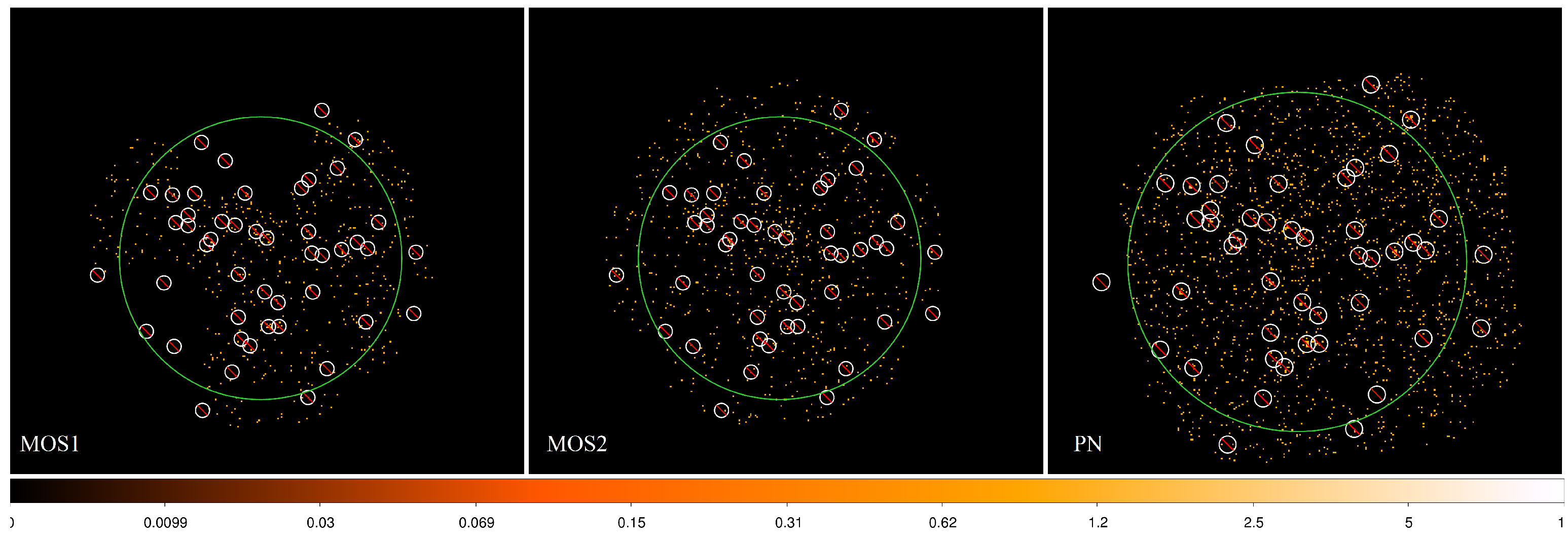
Abstract
:1. Introduction
2. Methods
2.1. XMM–Newton Data Analysis
2.2. Lin’s Magnetopause Model
3. Results
3.1. Solar Wind and Geomagnetic Conditions
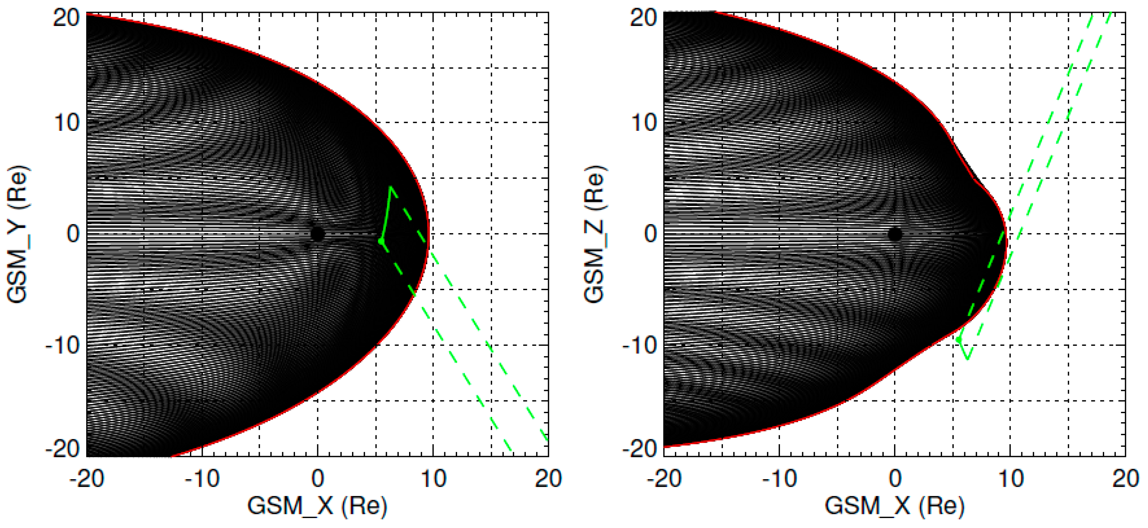
3.2. Line of Sight
3.3. SWCX Soft X-Ray Emission
3.4. Observational Geometric Relationship
3.5. Tangent Direction of Magnetopause
4. Conclusions
Author Contributions
Funding
Institutional Review Board Statement
Informed Consent Statement
Data Availability Statement
Acknowledgments
Conflicts of Interest
Abbreviations
| SWCX | Solar wind charge exchange |
| SMILE | Solar wind Magnetospheric Ionosphere Link Explorer |
Appendix A. Initial Data Processing
References
- Branduardi-Raymont, G.; Sembay, S.F.; Eastwood, J.P.; Sibeck, D.G.; Abbey, T.A.; Brown, P.; Carter, J.A.; Carr, C.M.; Forsyth, C.; Kataria, D.; et al. AXIOM: Advanced X-ray imaging of the magnetosphere. Exp. Astron. Vol. 2012, 33, 403–443. [Google Scholar] [CrossRef] [Green Version]
- Collier, M.; Porter, F.; Sibeck, D.; Carter, J.; Chiao, M.; Chornay, D.; Cravens, T.; Galeazzi, M.; Keller, J.; Koutroumpa, D.; et al. Prototyping a global soft X-ray imaging instrument for heliophysics, planetary science, and astrophysics science. Astron. Nachrichten 2012, 333, 378–382. [Google Scholar] [CrossRef] [Green Version]
- Walsh, B.M.; Collier, M.R.; Kuntz, K.D.; Porter, F.S.; Sibeck, D.G.; Snowden, S.L.; Carter, J.A.; Collado-Vega, Y.; Connor, H.K.; Cravens, T.E.; et al. Wide field-of-view soft X-ray imaging for solar wind-magnetosphere interactions. J. Geophys. Res. Space Phys. 2016, 121, 3353–3361. [Google Scholar] [CrossRef] [Green Version]
- Sibeck, D.G.; Allen, R.; Aryan, H.; Bodewits, D.; Brandt, P.; Branduardi-Raymont, G.; Brown, G.; Carter, J.A.; Collado-Vega, Y.M.; Collier, M.R.; et al. Imaging Plasma Density Structures in the Soft X-Rays Generated by Solar Wind Charge Exchange with Neutrals. Space Sci. Rev. 2018, 214, 79. [Google Scholar] [CrossRef] [Green Version]
- Cravens, T.E. Comet Hyakutake x-ray source: Charge transfer of solar wind heavy ions. Geophys. Res. Lett. 1997, 24, 105–108. [Google Scholar] [CrossRef]
- Lisse, C.M.; Dennerl, K.; Englhauser, J.; Harden, M.; Marshall, F.E.; Mumma, M.J.; Petre, R.; Pye, J.P.; Ricketts, M.J.; Schmitt, J.; et al. Discovery of X-ray and Extreme Ultraviolet Emission from Comet C/Hyakutake 1996 B2. Science 1996, 274, 205–209. [Google Scholar] [CrossRef] [Green Version]
- Wargelin, B.J.; Markevitch, M.; Juda, M.; Kharchenko, V.; Edgar, R.; Dalgarno, A.A. Chandra observations of the “dark” Moon and geocoronal solar wind charge transfer. Astrophys. J. 2004, 607, 596–610. [Google Scholar] [CrossRef]
- Branduardi-Raymont, G.; Elsner, R.F.; Gladstone, G.R.; Ramsay, G.; Rodriguez, P.; Soria, R.; Waite, J.H. First observation of Jupiter by XMM–Newton. A&A 2004, 424, 331–337. [Google Scholar] [CrossRef] [Green Version]
- Dennerl, K.; Lisse, C.M.; Bhardwaj, A.; Burwitz, V.; Englhauser, J.; Gunell, H.; Holmström, M.; Jansen, F.; Kharchenko, V.; Rodríguez-Pascual, P.M. First observation of Mars with XMM–Newton-High resolution X-ray spectroscopy with RGS. A&A 2006, 451, 709–722. [Google Scholar] [CrossRef] [Green Version]
- Dennerl, K. X-rays from Venus observed with Chandra. Planet. Space Sci. 2008, 56, 1414–1423. [Google Scholar] [CrossRef]
- Collier, M.R.; Snowden, S.L.; Sarantos, M.; Benna, M.; Carter, J.A.; Cravens, T.E.; Farrell, W.M.; Fatemi, S.; Hills, H.K.; Hodges, R.R.; et al. On lunar exospheric column densities and solar wind access beyond the terminator from ROSAT soft X-ray observations of solar wind charge exchange. J. Geophys. Res. Planets 2014, 119, 1459–1478. [Google Scholar] [CrossRef] [Green Version]
- Galeazzi, M.; Chiao, M.; Collier, M.R.; Cravens, T.; Koutroumpa, D.; Kuntz, K.D.; Lallement, R.; Lepri, S.T.; McCammon, D.; Morgan, K.; et al. The origin of the local 1/4-keV X-ray flux in both charge exchange and a hot bubble. Nature 2014, 512, 171–173. [Google Scholar] [CrossRef] [PubMed] [Green Version]
- Snowden, S.L.; Collier, M.R.; Kuntz, K.D. XMM–Newton Observation of Solar Wind Charge Exchange Emission. Astrophys. J. 2004, 610, 1182–1190. [Google Scholar] [CrossRef] [Green Version]
- Fujimoto, R.; Mitsuda, K.; McCammon, D.; Takei, Y.; Bauer, M.; Ishisaki, Y.; Porter, F.S.; Yamaguchi, H.; Hayashida, K.; Yamasaki, N.Y. Evidence for Solar-Wind Charge-Exchange X-Ray Emission from the Earth’s Magnetosheath. Prog. Theor. Phys. Suppl. 2007, 169, 71–74. [Google Scholar] [CrossRef] [Green Version]
- Carter, J.A.; Sembay, S. Identifying XMM–Newton observations affected by solar wind charge exchange. Part I. A&A 2008, 489, 837–848. [Google Scholar] [CrossRef] [Green Version]
- Kuntz, K.D.; Snowden, S.L. The X-Ray-Emitting Components toward l=111∘: The Local Hot Bubble and Beyond. Astrophys. J. 2008, 674, 209–219. [Google Scholar] [CrossRef]
- Snowden, S.L.; Collier, M.R.; Cravens, T.; Kuntz, K.D.; Lepri, S.T.; Robertson, I.; Tomas, L. Observation of solar wind charge exchange emission from exospheric material in and outside Earth’s magnetosheath 2008 september 25. Astrophys. J. 2009, 691, 372. [Google Scholar] [CrossRef]
- Carter, J.A.; Sembay, S.; Read, A.M. A high charge state coronal mass ejection seen through solar wind charge exchange emission as detected by XMM–Newton. Mon. Not. R. Astron. Soc. 2010, 402, 867–878. [Google Scholar] [CrossRef] [Green Version]
- Ezoe, Y.; Ebisawa, K.; Yamasaki, N.Y.; Mitsuda, K.; Yoshitake, H.; Terada, N.; Miyoshi, Y.; Fujimoto, R. Time Variability of the Geocoronal Solar-Wind Charge Exchange in the Direction of the Celestial Equator. Publ. Astron. Soc. Jpn. 2010, 62, 981–986. [Google Scholar] [CrossRef] [Green Version]
- Carter, J.A.; Sembay, S.; Read, A.M. Identifying XMM–Newton observations affected by solar wind charge exchange—Part II. A&A 2011, 527, A115. [Google Scholar] [CrossRef] [Green Version]
- Ezoe, Y.; Miyoshi, Y.; Yoshitake, H.; Mitsuda, K.; Terada, N.; Oishi, S.; Ohashi, T. Enhancement of Terrestrial Diffuse X-Ray Emission Associated with Coronal Mass Ejection and Geomagnetic Storm. Publ. Astron. Soc. Jpn. 2011, 63, S691–S704. [Google Scholar] [CrossRef] [Green Version]
- Carter, J.; Sembay, S.; Read, A. Exospheric solar wind charge exchange as seen by XMM–Newton. Astron. Nachrichten 2012, 333, 313–318. [Google Scholar] [CrossRef]
- Ishikawa, K.; Ezoe, Y.; Miyoshi, Y.; Terada, N.; Mitsuda, K.; Ohashi, T. Suzaku Observation of Strong Solar-Wind Charge-Exchange Emission from the Terrestrial Exosphere during a Geomagnetic Storm. Publ. Astron. Soc. Jpn. 2013, 65, 63. [Google Scholar] [CrossRef] [Green Version]
- Wargelin, B.J.; Kornbleuth, M.; Martin, P.L.; Juda, M. Observation and modeling of geocoronal charge exchange X-ray emission during solar wind gusts. Astrophys. J. 2014, 796, 28. [Google Scholar] [CrossRef] [Green Version]
- Kuntz, K.D.; Collado-Vega, Y.M.; Collier, M.R.; Connor, H.K.; Cravens, T.E.; Koutroumpa, D.; Porter, F.S.; Robertson, I.P.; Sibeck, D.G.; Snowden, S.L.; et al. The solar wind charge-exchange production factor for Hydrogen. Astrophys. J. 2015, 808, 143. [Google Scholar] [CrossRef] [Green Version]
- Ishi, D.; Ishikawa, K.; Numazawa, M.; Miyoshi, Y.; Terada, N.; Mitsuda, K.; Ohashi, T.; Ezoe, Y. Suzaku detection of enigmatic geocoronal solar wind charge exchange event associated with coronal mass ejection. Publ. Astron. Soc. Jpn. 2019, 71, 23. [Google Scholar] [CrossRef]
- Asakura, K.; Matsumoto, H.; Okazaki, K.; Yoneyama, T.; Noda, H.; Hayashida, K.; Tsunemi, H.; Nakajima, H.; Katsuda, S.; Ishi, D.; et al. Suzaku detection of solar wind charge exchange emission from a variety of highly ionized ions in an interplanetary coronal mass ejection. Publ. Astron. Soc. Jpn. 2021, 73, 504–518. [Google Scholar] [CrossRef]
- Zhang, Y.; Sun, T.; Wang, C.; Ji, L.; Carter, J.A.; Sembay, S.; Koutroumpa, D.; Liu, Y.D.; Liang, G.; Liu, W.; et al. Solar Wind Charge Exchange Soft X-Ray Emissions in the Magnetosphere during an Interplanetary Coronal Mass Ejection Compared to Its Driven Sheath. Astrophys. J. Lett. 2022, 932, L1. [Google Scholar] [CrossRef]
- Branduardi-Raymont, G.; Wang, G.C.; Escoubet, C.; Adamovic, M.; Agnolon, D.; Berthomier, M.; Carter, J.; Chen, W.; Colangeli, L.; Collier, M.; et al. SMILE definition study report (Red Book). In SMILE Definition Study Report, European Space Agency, ESA/SCI; 2018; pp. 1–86. [Google Scholar] [CrossRef]
- Wang, C.; Branduardi-Raymont, G. Update on the ESA-CAS Joint Solar Wind Magnetosphere Ionosphere Link Explorer(SMILE)Mission. Chin. J. Space Sci. 2020, 40, 700–703. [Google Scholar] [CrossRef]
- Wang, C.; Sun, T. Methods to derive the magnetopause from soft X-ray images by the SMILE mission. Geosci. Lett. 2022, 9, 30. [Google Scholar] [CrossRef]
- Collier, M.R.; Connor, H.K. Magnetopause Surface Reconstruction From Tangent Vector Observations. J. Geophys. Res. Space Phys. 2018, 123, 10,189–10,199. [Google Scholar] [CrossRef] [Green Version]
- Jorgensen, A.M.; Sun, T.; Wang, C.; Dai, L.; Sembay, S.; Wei, F.; Guo, Y.; Xu, R. Boundary Detection in Three Dimensions With Application to the SMILE Mission: The Effect of Photon Noise. J. Geophys. Res. Space Phys. 2019, 124, 4365–4383. [Google Scholar] [CrossRef] [Green Version]
- Jorgensen, A.M.; Sun, T.; Wang, C.; Dai, L.; Sembay, S.; Zheng, J.; Yu, X. Boundary Detection in Three Dimensions With Application to the SMILE Mission: The Effect of Model-Fitting Noise. J. Geophys. Res. Space Phys. 2019, 124, 4341–4355. [Google Scholar] [CrossRef]
- Sun, T.; Wang, C.; Connor, H.K.; Jorgensen, A.M.; Sembay, S. Deriving the Magnetopause Position from the Soft X-Ray Image by Using the Tangent Fitting Approach. J. Geophys. Res. Space Phys. 2020, 125, e2020JA028169. [Google Scholar] [CrossRef]
- Jorgensen, A.M.; Xu, R.; Sun, T.; Huang, Y.; Li, L.; Dai, L.; Wang, C. A Theoretical Study of the Tomographic Reconstruction of Magnetosheath X-Ray Emissions. J. Geophys. Res. Space Phys. 2022, 127, e2021JA029948. [Google Scholar] [CrossRef]
- Sun, T.R.; Wang, C.; Sembay, S.F.; Lopez, R.E.; Escoubet, C.P.; Branduardi-Raymont, G.; Zheng, J.H.; Yu, X.Z.; Guo, X.C.; Dai, L.; et al. Soft X-ray Imaging of the Magnetosheath and Cusps Under Different Solar Wind Conditions: MHD Simulations. J. Geophys. Res. Space Phys. 2019, 124, 2435–2450. [Google Scholar] [CrossRef] [Green Version]
- Samsonov, A.; Carter, J.A.; Read, A.; Sembay, S.; Branduardi-Raymont, G.; Sibeck, D.; Escoubet, P. Finding Magnetopause Standoff Distance Using a Soft X-Ray Imager: 1. Magnetospheric Masking. J. Geophys. Res. Space Phys. 2022, 127, e2022JA030848. [Google Scholar] [CrossRef]
- Lin, R.L.; Zhang, X.X.; Liu, S.Q.; Wang, Y.L.; Gong, J.C. A three-dimensional asymmetric magnetopause model. J. Geophys. Res. Space Phys. 2010, 115, A04207. [Google Scholar] [CrossRef]
- Lepri, S.T.; Landi, E.; Zurbuchen, T.H. Solar wind heavy ions over solar cycle 23: ACE/SWICS measurements. Astrophys. J. 2013, 768, 94. [Google Scholar] [CrossRef]
- Guo, Y.; Sun, T.; Wang, C.; Sembay, S. Deriving the magnetopause position from wide field-of-view soft X-ray imager simulation. Sci. China Earth Sci. 2022, 65, 1601–1611. [Google Scholar] [CrossRef]
- Kuntz, K.D.; Snowden, S.L. The EPIC-MOS particle-induced background spectra. A&A 2008, 478, 575–596. [Google Scholar] [CrossRef]


Disclaimer/Publisher’s Note: The statements, opinions and data contained in all publications are solely those of the individual author(s) and contributor(s) and not of MDPI and/or the editor(s). MDPI and/or the editor(s) disclaim responsibility for any injury to people or property resulting from any ideas, methods, instructions or products referred to in the content. |
© 2023 by the authors. Licensee MDPI, Basel, Switzerland. This article is an open access article distributed under the terms and conditions of the Creative Commons Attribution (CC BY) license (https://creativecommons.org/licenses/by/4.0/).
Share and Cite
Zhang, Y.; Sun, T.; Carter, J.A.; Liu, W.; Sembay, S.; Ji, L.; Wang, C. The Relationship between Solar Wind Charge Exchange Soft X-ray Emission and the Tangent Direction of Magnetopause in an XMM–Newton Event. Magnetochemistry 2023, 9, 88. https://doi.org/10.3390/magnetochemistry9040088
Zhang Y, Sun T, Carter JA, Liu W, Sembay S, Ji L, Wang C. The Relationship between Solar Wind Charge Exchange Soft X-ray Emission and the Tangent Direction of Magnetopause in an XMM–Newton Event. Magnetochemistry. 2023; 9(4):88. https://doi.org/10.3390/magnetochemistry9040088
Chicago/Turabian StyleZhang, Yingjie, Tianran Sun, Jennifer A. Carter, Wenhao Liu, Steve Sembay, Li Ji, and Chi Wang. 2023. "The Relationship between Solar Wind Charge Exchange Soft X-ray Emission and the Tangent Direction of Magnetopause in an XMM–Newton Event" Magnetochemistry 9, no. 4: 88. https://doi.org/10.3390/magnetochemistry9040088