
Modeling of the Magnetic Turbulence Level and Source Function of Particle Injection from Multiple SEP Events

Abstract
:1. Introduction
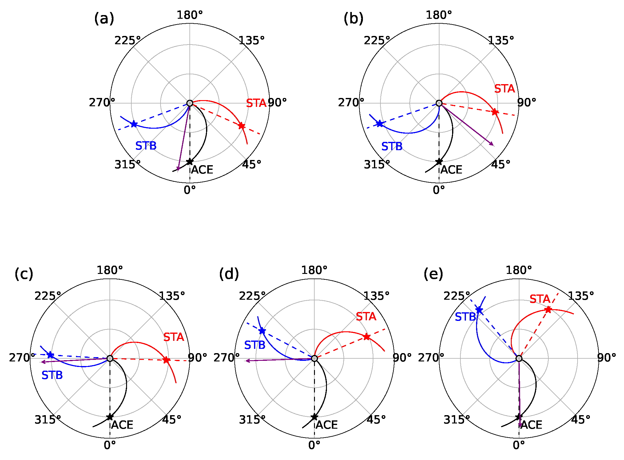
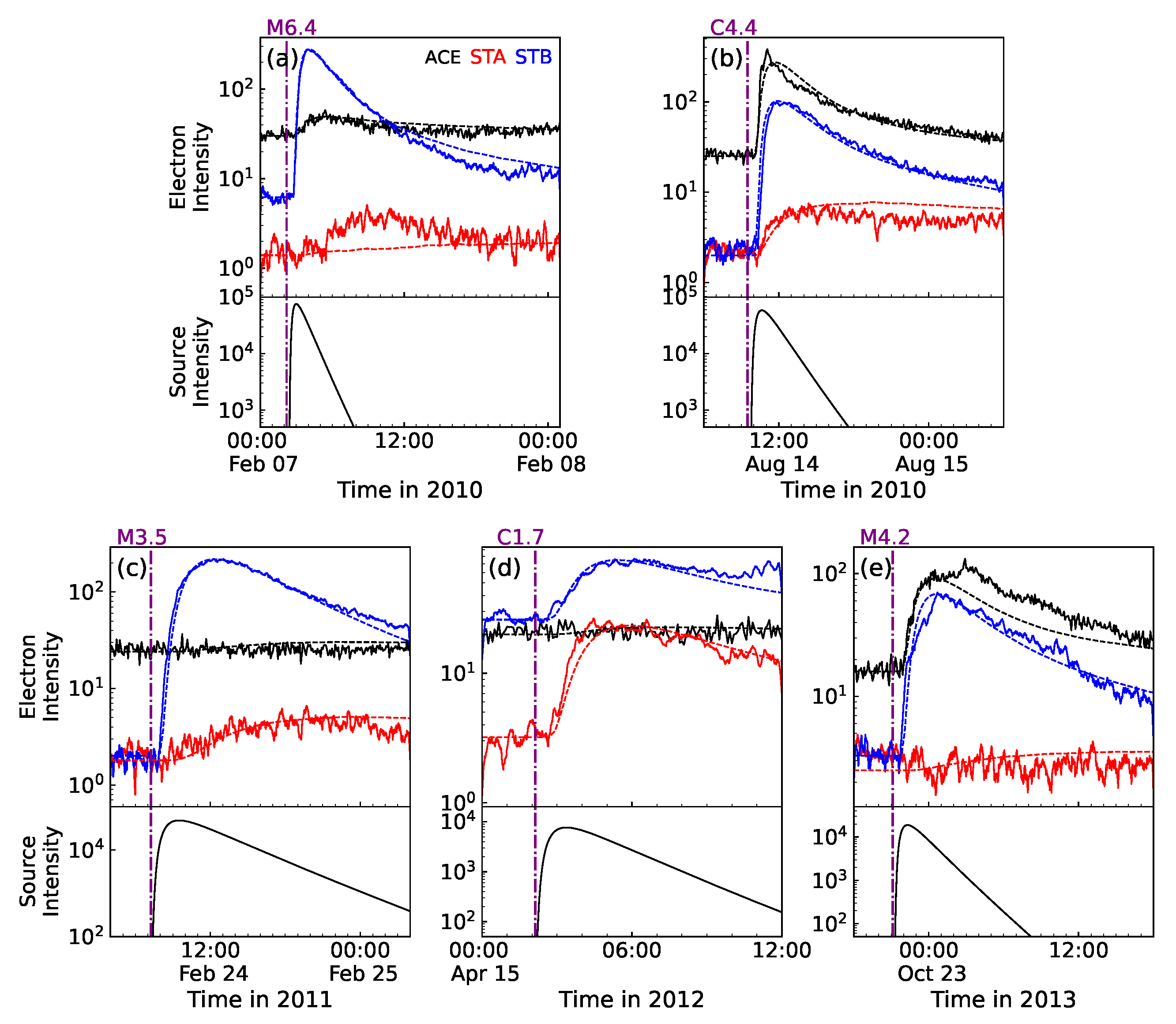
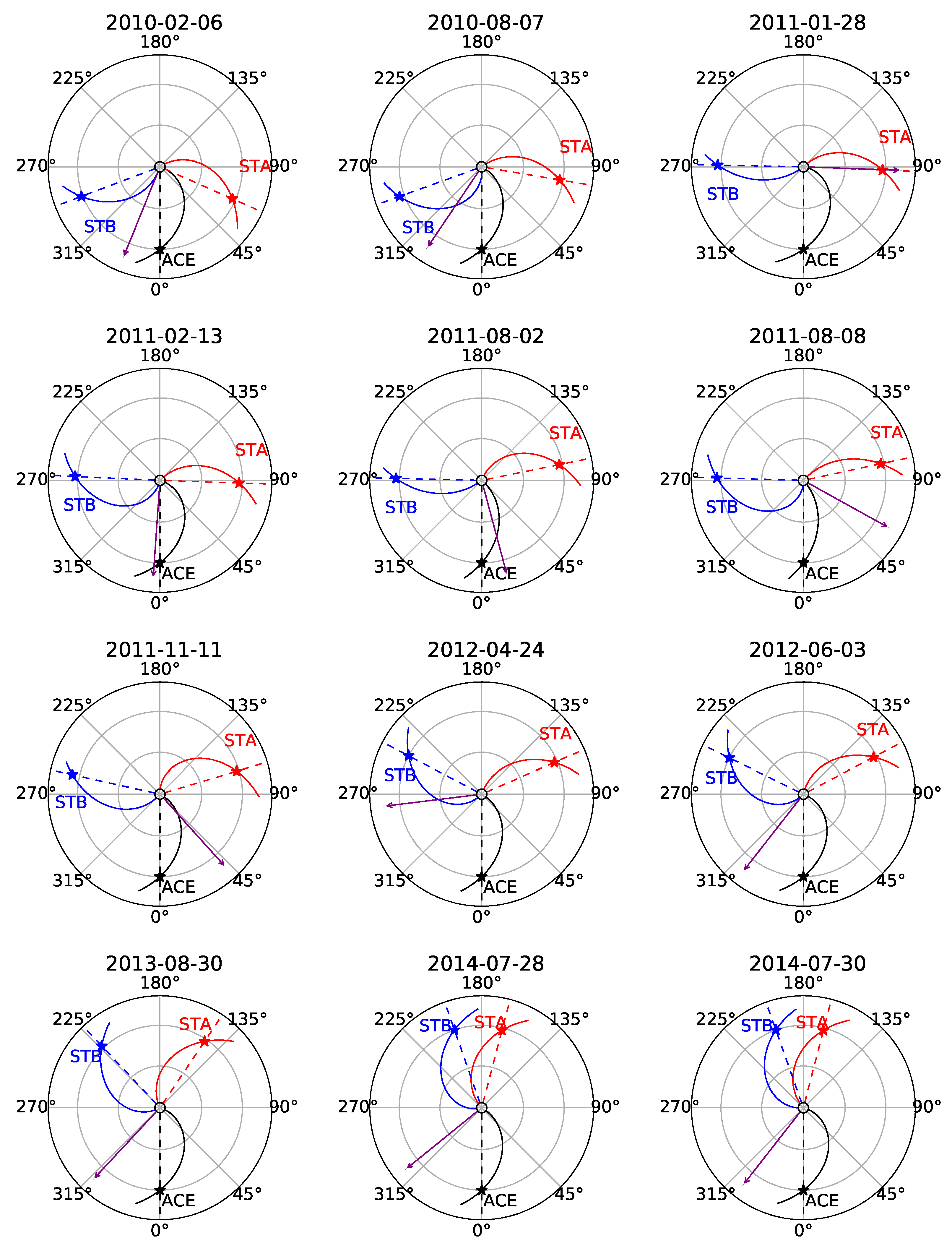
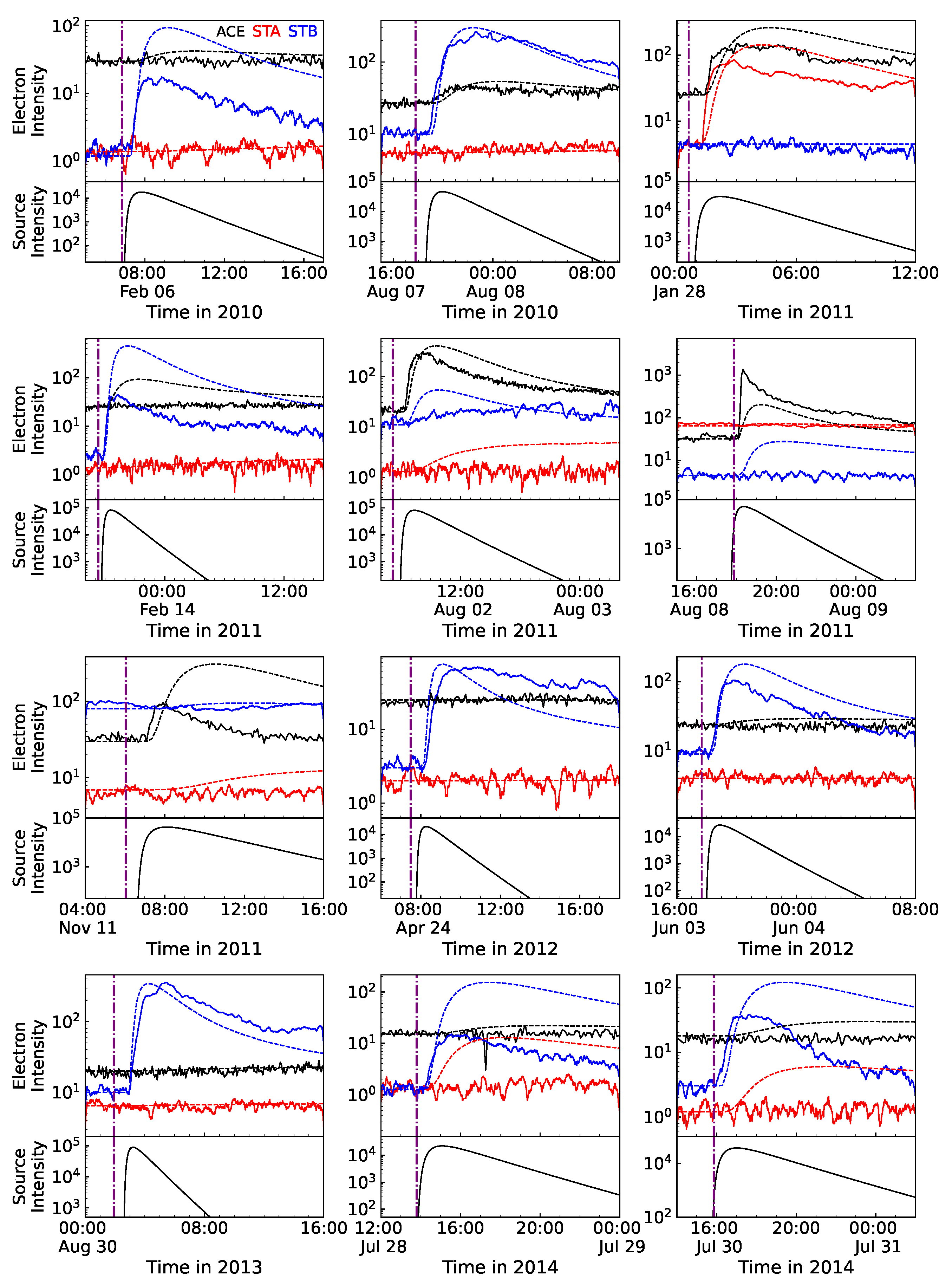
2. Data
3. SEP Transport Model
3.1. Focused Transport Equation
3.2. Diffusion Coefficients
3.3. Source Function of Particle Injection
4. Best-Fit Simulation Results for SEP Events in Group I
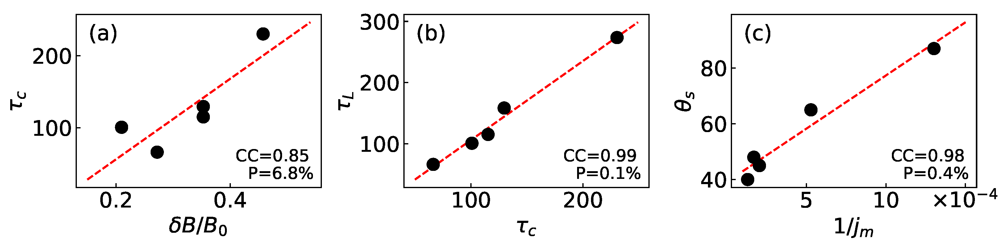
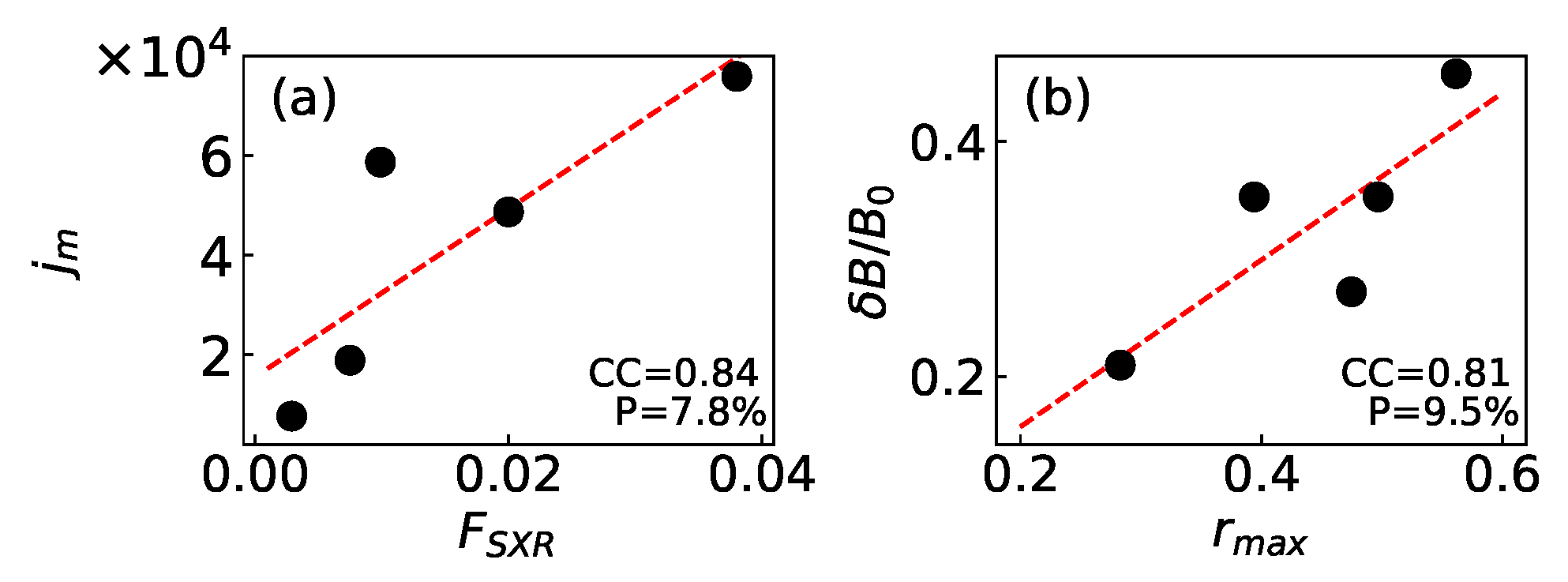
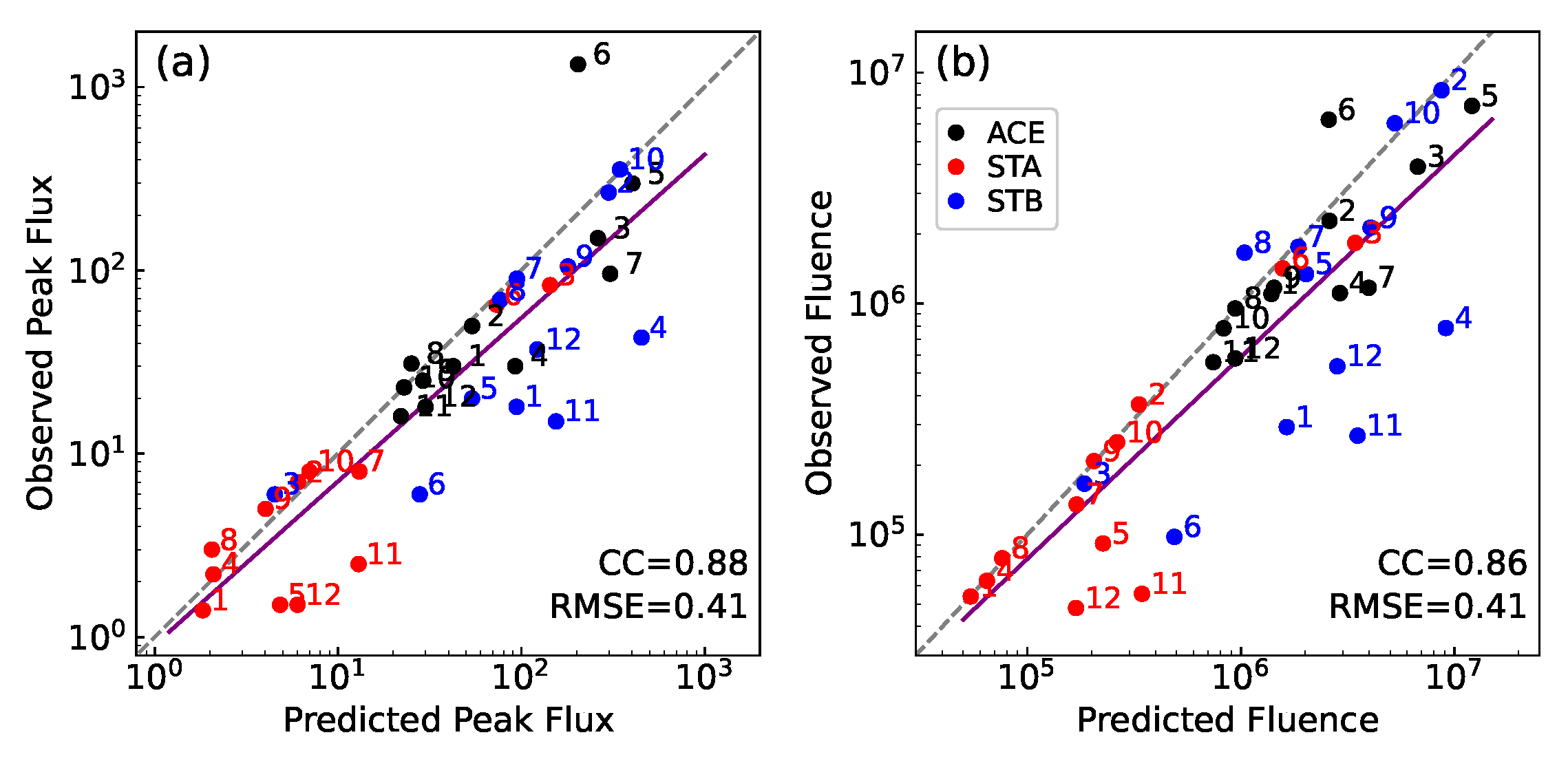
5. Model for Key Parameters
5.1. Correlations among the Key Parameters
5.2. Models for the Best-Fit Key Parameters
6. Simulation Results for SEP Events in Group II without Fitting
7. Conclusions and Discussion
Author Contributions
Funding
Institutional Review Board Statement
Informed Consent Statement
Data Availability Statement
Acknowledgments
Conflicts of Interest
References
- Lanzerotti, L.J. Space Weather: Historical and Contemporary Perspectives. Space Sci. Rev. 2017, 212, 1253–1270. [Google Scholar] [CrossRef] [Green Version]
- Mertens, C.J.; Slaba, T.C.; Hu, S. Active Dosimeter-Based Estimate of Astronaut Acute Radiation Risk for Real-Time Solar Energetic Particle Events. Space Weather 2018, 16, 1291–1316. [Google Scholar] [CrossRef]
- Posner, A. Up to 1-hour forecasting of radiation hazards from solar energetic ion events with relativistic electrons. Space Weather 2007, 5, 05001. [Google Scholar] [CrossRef] [Green Version]
- Kallenrode, M.B. Current views on impulsive and gradual solar energetic particle events. J. Phys. Nucl. Phys. 2003, 29, 965–981. [Google Scholar] [CrossRef]
- Reames, D.V. Particle acceleration at the Sun and in the heliosphere. Space Sci. Rev. 1999, 90, 413–491. [Google Scholar] [CrossRef]
- Reames, D.V. The Two Sources of Solar Energetic Particles. Space Sci. Rev. 2013, 175, 53–92. [Google Scholar] [CrossRef] [Green Version]
- Cliver, E.W.; Ling, A.G.; Belov, A.; Yashiro, S. Size distributions of solar flares and solar energetic particle events. Astrophys. Lett. 2012, 756, L29. [Google Scholar] [CrossRef]
- Park, J.; Moon, Y.J.; Lee, D.H.; Youn, S. Dependence of solar proton events on their associated activities: Flare parameters. J. Geophys. Res. (Space Phys.) 2010, 115, A10105. [Google Scholar] [CrossRef] [Green Version]
- Kurt, V.; Belov, A.; Mavromichalaki, H.; Gerontidou, M. Statistical analysis of solar proton events. Ann. Geophys. 2004, 22, 2255–2271. [Google Scholar] [CrossRef] [Green Version]
- Wu, S.S.; Qin, G. Model of Energy Spectrum Parameters of Ground Level Enhancement Events in Solar Cycle 23. J. Geophys. Res. (Space Phys.) 2018, 123, 76–92. [Google Scholar] [CrossRef] [Green Version]
- Gopalswamy, N.; Yashiro, S.; Akiyama, S.; Mäkelä, P.; Xie, H.; Kaiser, M.L.; Howard, R.A.; Bougeret, J.L. Coronal mass ejections, type II radio bursts, and solar energetic particle events in the SOHO era. Ann. Geophys. 2008, 26, 3033–3047. [Google Scholar] [CrossRef]
- Kahler, S.W. The correlation between solar energetic particle peak intensities and speeds of coronal mass ejections: Effects of ambient particle intensities and energy spectra. J. Geophys. Res. (Space Phys.) 2001, 106, 20947–20956. [Google Scholar] [CrossRef]
- Park, J.; Moon, Y.J.; Gopalswamy, N. Dependence of solar proton events on their associated activities: Coronal mass ejection parameters. J. Geophys. Res. (Space Phys.) 2012, 117, A08108. [Google Scholar] [CrossRef] [Green Version]
- Cane, H.V.; Richardson, I.G.; von Rosenvinge, T.T. A study of solar energetic particle events of 1997-2006: Their composition and associations. J. Geophys. Res. (Space Phys.) 2010, 115, A08101. [Google Scholar] [CrossRef]
- Dierckxsens, M.; Tziotziou, K.; Dalla, S.; Patsou, I.; Marsh, M.S.; Crosby, N.B.; Malandraki, O.; Tsiropoula, G. Relationship between Solar Energetic Particles and Properties of Flares and CMEs: Statistical Analysis of Solar Cycle 23 Events. Sol. Phys. 2015, 290, 841–874. [Google Scholar] [CrossRef] [Green Version]
- Ding, L.G.; Jiang, Y.; Li, G. Are There Two Distinct Solar Energetic Particle Releases in the 2012 May 17 Ground Level Enhancement Event? Astrophys. J. 2016, 818, 169. [Google Scholar] [CrossRef]
- Miteva, R.; Klein, K.L.; Malandraki, O.; Dorrian, G. Solar Energetic Particle Events in the 23rd Solar Cycle: Interplanetary Magnetic Field Configuration and Statistical Relationship with Flares and CMEs. Sol. Phys. 2013, 282, 579–613. [Google Scholar] [CrossRef] [Green Version]
- Richardson, I.G.; Von Rosenvinge, T.T.; Cane, H.V.; Christian, E.R.; Cohen, C.M.S.; Labrador, A.W.; Leske, R.A.; Mewaldt, R.A.; Wiedenbeck, M.E.; Stone, E.C. >25 MeV Proton Events Observed by the High Energy Telescopes on the STEREO A and B Spacecraft and/or at Earth During the First ∼Seven Years of the STEREO Mission. Sol. Phys. 2014, 289, 3059–3107. [Google Scholar] [CrossRef]
- Lario, D.; Aran, A.; Gómez-Herrero, R.; Dresing, N.; Heber, B.; Ho, G.C.; Decker, R.B.; Roelof, E.C. Longitudinal and Radial Dependence of Solar Energetic Particle Peak Intensities: STEREO, ACE, SOHO, GOES, and MESSENGER Observations. Astrophys. J. 2013, 767, 41. [Google Scholar] [CrossRef]
- Dresing, N.; Gómez-Herrero, R.; Heber, B.; Klassen, A.; Malandraki, O.; Dröge, W.; Kartavykh, Y. Statistical survey of widely spread out solar electron events observed with STEREO and ACE with special attention to anisotropies. Astron. Astrophys. 2014, 567, A27. [Google Scholar] [CrossRef]
- Paassilta, M.; Papaioannou, A.; Dresing, N.; Vainio, R.; Valtonen, E.; Heber, B. Catalogue of >55 MeV Wide-longitude Solar Proton Events Observed by SOHO, ACE, and the STEREOs at ∼1 AU During 2009-2016. Sol. Phys. 2018, 293, 70. [Google Scholar] [CrossRef] [Green Version]
- Adhikari, L.; Zank, G.P.; Zhao, L.L.; Kasper, J.C.; Korreck, K.E.; Stevens, M.; Case, A.W.; Whittlesey, P.; Larson, D.; Livi, R.; et al. Turbulence Transport Modeling and First Orbit Parker Solar Probe (PSP) Observations. Astrophys. J. Suppl. Ser. 2020, 246, 38. [Google Scholar] [CrossRef] [Green Version]
- McKibben, R.B. Observations of Solar Proton Events Made from Very Widely Separated Spacecraft. Bull. Am. Astron. Soc. 1972, 4, 387. [Google Scholar]
- Reames, D.V.; Barbier, L.M.; Ng, C.K. The Spatial Distribution of Particles Accelerated by Coronal Mass Ejection-Driven Shocks. Astrophys. J. 1996, 466, 473. [Google Scholar] [CrossRef]
- Lario, D.; Kallenrode, M.B.; Decker, R.B.; Roelof, E.C.; Krimigis, S.M.; Aran, A.; Sanahuja, B. Radial and Longitudinal Dependence of Solar 4-13 MeV and 27-37 MeV Proton Peak Intensities and Fluences: Helios and IMP 8 Observations. Astrophys. J. 2006, 653, 1531–1544. [Google Scholar] [CrossRef] [Green Version]
- Qin, G.; Zhang, M.; Dwyer, J.R. Effect of adiabatic cooling on the fitted parallel mean free path of solar energetic particles. J. Geophys. Res. (Space Phys.) 2006, 111, A08101. [Google Scholar] [CrossRef] [Green Version]
- Wang, Y.; Qin, G.; Zhang, M. Effects of perpendicular diffusion on energetic particles accelerated by the interplanetary coronal mass ejection shock. Astrophys. J. 2012, 752, 37. [Google Scholar] [CrossRef] [Green Version]
- Qin, G.; Wang, Y.; Zhang, M.; Dalla, S. Transport of Solar Energetic Particles Accelerated by ICME Shocks: Reproducing the Reservoir Phenomenon. Astrophys. J. 2013, 766, 74. [Google Scholar] [CrossRef] [Green Version]
- Wang, Y.; Qin, G.; Zhang, M.; Dalla, S. A Numerical Simulation of Solar Energetic Particle Dropouts during Impulsive Events. Astrophys. J. 2014, 789, 157. [Google Scholar] [CrossRef] [Green Version]
- Dröge, W.; Kartavykh, Y.Y.; Dresing, N.; Heber, B.; Klassen, A. Wide longitudinal distribution of interplanetary electrons following the 7 February 2010 solar event: Observations and transport modeling. J. Geophys. Res. (Space Phys.) 2014, 119, 6074–6094. [Google Scholar] [CrossRef]
- Qin, G.; Wang, Y. Simulations of a gradual solar energetic particle event observed by HELIOS 1, HELIOS 2, and IMP 8. Astrophys. J. 2015, 809, 177. [Google Scholar] [CrossRef] [Green Version]
- Wang, Y.; Qin, G. Simulations of the spatial and temporal invariance in the spectra of gradual solar energetic particle events. Astrophys. J. 2015, 806, 252. [Google Scholar] [CrossRef] [Green Version]
- Lario, D.; Kwon, R.Y.; Richardson, I.G.; Raouafi, N.E.; Thompson, B.J.; Von Rosenvinge, T.T.; Mays, M.L.; Mäkelä, P.A.; Xie, H.; Bain, H.M.; et al. The Solar Energetic Particle Event of 2010 August 14: Connectivity with the Solar Source Inferred from Multiple Spacecraft Observations and Modeling. Astrophys. J. 2017, 838, 51. [Google Scholar] [CrossRef] [Green Version]
- Lian, L.L.; Qin, G.; Wang, Y.; Cui, S.W. Observations and numerical simulations of gradual SEP events with Ulysses and ACE. In Proceedings of the 37th International Cosmic Ray Conference, Berlin, Germany, 12–23 July 2021; Volume 395, p. 1351. [Google Scholar] [CrossRef]
- Zhang, M.; Qin, G.; Rassoul, H. Propagation of solar energetic particles in three-dimensional interplanetary magnetic fields. Astrophys. J. 2009, 692, 109. [Google Scholar] [CrossRef] [Green Version]
- Dröge, W.; Kartavykh, Y.Y.; Klecker, B.; Kovaltsov, G.A. Anisotropic Three-Dimensional Focused Transport of Solar Energetic Particles in the Inner Heliosphere. Astrophys. J. 2010, 709, 912–919. [Google Scholar] [CrossRef]
- Dresing, N.; Gómez-Herrero, R.; Klassen, A.; Heber, B.; Kartavykh, Y.; Dröge, W. The Large Longitudinal Spread of Solar Energetic Particles During the 17 January 2010 Solar Event. Sol. Phys. 2012, 281, 281–300. [Google Scholar] [CrossRef] [Green Version]
- Dröge, W.; Kartavykh, Y.Y.; Dresing, N.; Klassen, A. Multi-spacecraft Observations and Transport Modeling of Energetic Electrons for a Series of Solar Particle Events in August 2010. Astrophys. J. 2016, 826, 134. [Google Scholar] [CrossRef] [Green Version]
- Wu, S.S.; Qin, G. Magnetic Cloud and Sheath in the Ground-level Enhancement Event of 2000 July 14. I. Effects on the Solar Energetic Particles. Astrophys. J. 2020, 904, 151. [Google Scholar] [CrossRef]
- Mazur, J.E.; Mason, G.M.; Dwyer, J.R.; Giacalone, J.; Jokipii, J.R.; Stone, E.C. Interplanetary Magnetic Field Line Mixing Deduced from Impulsive Solar Flare Particles. Astrophys. J. 2000, 532, L79. [Google Scholar] [CrossRef] [Green Version]
- Gosling, J.T.; de Koning, C.A.; Skoug, R.M.; Steinberg, J.T.; McComas, D.J. Dispersionless modulations in low-energy solar electron bursts and discontinuous changes in the solar wind electron strahl. J. Geophys. Res. Space Phys. 2004, 109, A05102. [Google Scholar] [CrossRef]
- Trenchi, L.; Bruno, R.; Telloni, D.; D’amicis, R.; Marcucci, M.F.; Zurbuchen, T.H.; Weberg, M. Solar Energetic Particle Modulations Associated with Coherent Magnetic Structures. Astrophys. J. 2013, 770, 11. [Google Scholar] [CrossRef] [Green Version]
- Trenchi, L.; Bruno, R.; D’amicis, R.; Marcucci, M.F.; Telloni, D. Observations of IMF coherent structures and their relationship to SEP dropout events. Ann. Geophys. 2013b, 31, 1333. [Google Scholar] [CrossRef] [Green Version]
- Balch, C.C. SEC proton prediction model: Verification and analysis. Radiat. Meas. 1999, 30, 231–250. [Google Scholar] [CrossRef] [PubMed]
- Balch, C.C. Updated verification of the Space Weather Prediction Center’s solar energetic particle prediction model. Space Weather 2008, 6, S01001. [Google Scholar] [CrossRef]
- Núñez, M. Predicting solar energetic proton events (E > 10 MeV). Space Weather 2011, 9, S07003. [Google Scholar] [CrossRef]
- Núñez, M. Real-time prediction of the occurrence and intensity of the first hours of >100 MeV solar energetic proton events. Space Weather 2015, 13, 807–819. [Google Scholar] [CrossRef]
- Papaioannou, A.; Anastasiadis, A.; Sandberg, I.; Georgoulis, M.K.; Tsiropoula, G.; Tziotziou, K.; Jiggens, P.; Hilgers, A. A Novel Forecasting System for Solar Particle Events and Flares (FORSPEF). J. Phys. Conf. Ser. 2015, 632, 012075. [Google Scholar] [CrossRef]
- Papaioannou, A.; Anastasiadis, A.; Sandberg, I.; Jiggens, P. Nowcasting of Solar Energetic Particle Events using near real-time Coronal Mass Ejection characteristics in the framework of the FORSPEF tool. J. Space Weather Space Clim. 2018, 8, A37. [Google Scholar] [CrossRef]
- Alberti, T.; Laurenza, M.; Cliver, E.W.; Storini, M.; Consolini, G.; Lepreti, F. Solar Activity from 2006 to 2014 and Short-term Forecasts of Solar Proton Events Using the ESPERTA Model. Astrophys. J. 2017, 838, 59. [Google Scholar] [CrossRef]
- Laurenza, M.; Cliver, E.W.; Hewitt, J.; Storini, M.; Ling, A.G.; Balch, C.C.; Kaiser, M.L. A technique for short-term warning of solar energetic particle events based on flare location, flare size, and evidence of particle escape. Space Weather 2009, 7, S04008. [Google Scholar] [CrossRef] [Green Version]
- Kahler, S.W.; Cliver, E.W.; Ling, A.G. Validating the proton prediction system (PPS). J. Atmos.-Sol.-Terr. Phys. 2007, 69, 43–49. [Google Scholar] [CrossRef]
- Smart, D.F.; Shea, M.A. PPS-87: A new event oriented solar proton prediction model. Adv. Space Res. 1989, 9, 281–284. [Google Scholar] [CrossRef] [PubMed]
- Reid, G.C. A diffusive model for the initial phase of a solar proton event. J. Geophys. Res. (Space Phys.) 1964, 69, 2659–2667. [Google Scholar] [CrossRef]
- Zhao, L.L.; Zhang, M.; Lario, D. Modeling the Transport Processes of a Pair of Solar Energetic Particle Events Observed by Parker Solar Probe Near Perihelion. Astrophys. J. 2020, 898, 16. [Google Scholar] [CrossRef]
- Gold, R.E.; Krimigis, S.M.; Hawkins, S.E.; Haggerty, D.K.; Lohr, D.A.; Fiore, E.; Armstrong, T.P.; Holl, G.; Lanzerotti, L.J. Electron, Proton, and Alpha Monitor on the Advanced Composition Explorer spacecraft. Space Sci. Rev. 1998, 86, 541–562. [Google Scholar] [CrossRef]
- Müller-Mellin, R.; Böttcher, S.; Falenski, J.; Rode, E.; Duvet, L.; Sanderson, T.; Butler, B.; Johlander, B.; Smit, H. The Solar Electron and Proton Telescope for the STEREO Mission. Space Sci. Rev. 2008, 136, 363–389. [Google Scholar] [CrossRef]
- McComas, D.J.; Bame, S.J.; Barker, P.; Feldman, W.C.; Phillips, J.L.; Riley, P.; Griffee, J.W. Solar Wind Electron Proton Alpha Monitor (SWEPAM) for the Advanced Composition Explorer. Space Sci. Rev. 1998, 86, 563–612. [Google Scholar] [CrossRef]
- Galvin, A.B.; Kistler, L.M.; Popecki, M.A.; Farrugia, C.J.; Simunac, K.D.; Ellis, L.; Möbius, E.; Lee, M.A.; Boehm, M.; Carroll, J.; et al. The Plasma and Suprathermal Ion Composition (PLASTIC) Investigation on the STEREO Observatories. Space Sci. Rev. 2008, 136, 437–486. [Google Scholar] [CrossRef] [Green Version]
- Smith, C.W.; L’Heureux, J.; Ness, N.F.; Acuña, M.H.; Burlaga, L.F.; Scheifele, J. The ACE Magnetic Fields Experiment. Space Sci. Rev. 1998, 86, 613–632. [Google Scholar] [CrossRef]
- Skilling, J. Cosmic Rays in the Galaxy: Convection or Diffusion? Astrophys. J. 1971, 170, 265. [Google Scholar] [CrossRef]
- Beeck, J.; Wibberenz, G. Pitch Angle Distributions of Solar Energetic Particles and the Local Scattering Properties of the Interplanetary Medium. Astrophys. J. 1986, 311, 437–450. [Google Scholar] [CrossRef]
- Qin, G.; Zhang, M.; Dwyer, J.R.; Rassoul, H.K.; Mason, G.M. The Model Dependence of Solar Energetic Particle Mean Free Paths under Weak Scattering. Astrophys. J. 2005, 627, 562–566. [Google Scholar] [CrossRef]
- Qin, G.; Shalchi, A. Pitch-Angle Diffusion Coefficients of Charged Particles from Computer Simulations. Astrophys. J. 2009, 707, 61–66. [Google Scholar] [CrossRef]
- Qin, G.; Shalchi, A. Pitch-Angle Dependent Perpendicular Diffusion of Energetic Particles Interacting With Magnetic Turbulence. Appl. Phys. Res. 2014, 6, 1–13. [Google Scholar] [CrossRef] [Green Version]
- Earl, J.A. The diffusive idealization of charged-particle transport in random magnetic fields. Astrophys. J. 1974, 193, 231–242. [Google Scholar] [CrossRef] [Green Version]
- Jokipii, J.R. Cosmic-Ray Propagation. I. Charged Particles in a Random Magnetic Field. Astrophys. J. 1966, 146, 480. [Google Scholar] [CrossRef]
- Matthaeus, W.H.; Qin, G.; Bieber, J.W.; Zank, G.P. Nonlinear Collisionless Perpendicular Diffusion of Charged Particles. Astrophys. J. 2003, 590, L53–L56. [Google Scholar] [CrossRef] [Green Version]
- Shalchi, A.; Li, G.; Zank, G.P. Analytic forms of the perpendicular cosmic ray diffusion coefficient for an arbitrary turbulence spectrum and applications on transport of Galactic protons and acceleration at interplanetary shocks. Astrophys. Space Sci. 2010, 325, 99–111. [Google Scholar] [CrossRef]
- Matthaeus, W.H.; Goldstein, M.L.; Roberts, D.A. Evidence for the presence of quasi-two-dimensional nearly incompressible fluctuations in the solar wind. J. Geophys. Res. (Space Phys.) 1990, 95, 20673–20683. [Google Scholar] [CrossRef]
- Weygand, J.M.; Matthaeus, W.H.; Dasso, S.; Kivelson, M.G.; Kistler, L.M.; Mouikis, C. Anisotropy of the Taylor scale and the correlation scale in plasma sheet and solar wind magnetic field fluctuations. J. Geophys. Res. (Space Phys.) 2009, 114, 07213. [Google Scholar] [CrossRef]
- Weygand, J.M.; Matthaeus, W.H.; Dasso, S.; Kivelson, M.G. Correlation and Taylor scale variability in the interplanetary magnetic field fluctuations as a function of solar wind speed. J. Geophys. Res. (Space Phys.) 2011, 116, A08102. [Google Scholar] [CrossRef] [Green Version]
- Dröge, W. The Rigidity Dependence of Solar Particle Scattering Mean Free Paths. Astrophys. J. 2000, 537, 1073–1079. [Google Scholar] [CrossRef] [Green Version]
- Shalchi, A.; Qin, G. Random walk of magnetic field lines: Analytical theory versus simulations. Astrophys. Space Sci. 2010, 330, 279–287. [Google Scholar] [CrossRef]
- Zhang, M. A Markov Stochastic Process Theory of Cosmic-Ray Modulation. Astrophys. J. 1999, 513, 409. [Google Scholar] [CrossRef]
- Band, D.; Matteson, J.; Ford, L.; Schaefer, B.; Palmer, D.; Teegarden, B.; Cline, T.; Briggs, M.; Paciesas, W.; Pendleton, G.; et al. BATSE Observations of Gamma-Ray Burst Spectra. I. Spectral Diversity. Astrophys. J. 1993, 413, 281. [Google Scholar] [CrossRef]
- Qin, G.; Wu, S.S. A Model of Sunspot Number with a Modified Logistic Function. Astrophys. J. 2018, 869, 48. [Google Scholar] [CrossRef] [Green Version]
- Wu, S.S.; Qin, G. Predicting Sunspot Numbers for Solar Cycles 25 and 26. arXiv 2021, arXiv:2102.06001. [Google Scholar]
- Fox, N.J.; Velli, M.C.; Bale, S.D.; Decker, R.; Driesman, A.; Howard, R.A.; Kasper, J.C.; Kinnison, J.; Kusterer, M.; Lario, D.; et al. The Solar Probe Plus Mission: Humanity’s First Visit to Our Star. Space Sci. Rev. 2016, 204, 7–48. [Google Scholar] [CrossRef] [Green Version]
- McComas, D.J.; Alexander, N.; Angold, N.; Bale, S.; Beebe, C.; Birdwell, B.; Boyle, M.; Burgum, J.M.; Burnham, J.A.; Christian, E.R.; et al. Integrated Science Investigation of the Sun (ISIS): Design of the Energetic Particle Investigation. Space Sci. Rev. 2016, 204, 187–256. [Google Scholar] [CrossRef] [Green Version]
- Müller, D.; Cyr, O.S.; Zouganelis, I.; Gilbert, H.R.; Marsden, R.; Nieves-Chinchilla, T.; Antonucci, E.; Auchère, F.; Berghmans, D.; Horbury, T.S.; et al. The Solar Orbiter mission. Science overview. Astron. Astrophys. 2020, 642, A1. [Google Scholar] [CrossRef]
- Rodríguez-Pacheco, J.; Wimmer-Schweingruber, R.F.; Mason, G.M.; Ho, G.C.; Sánchez-Prieto, S.; Prieto, M.; Martín, C.; Seifert, H.; Andrews, G.B.; Kulkarni, S.R.; et al. The Energetic Particle Detector. Energetic particle instrument suite for the Solar Orbiter mission. Astron. Astrophys. 2020, 642, A7. [Google Scholar] [CrossRef] [Green Version]
- Jiang, C.; Wu, S.T.; Feng, X.; Hu, Q. Data-driven magnetohydrodynamic modelling of a flux-emerging active region leading to solar eruption. Nat. Commun. 2016, 7, 11522. [Google Scholar] [CrossRef] [PubMed] [Green Version]
- Qin, G.; Wu, S.S. Magnetic Cloud and Sheath in the Ground-level Enhancement Event of 2000 July 14. II. Effects on the Forbush Decrease. Astrophys. J. 2021, 908, 236. [Google Scholar] [CrossRef]
- Wijsen, N.; Samara, E.; Aran, A.; Lario, D.; Pomoell, J.; Poedts, S. A Self-consistent Simulation of Proton Acceleration and Transport Near a High-speed Solar Wind Stream. Astrophys. J. 2021, 908, L26. [Google Scholar] [CrossRef]
- Zhao, L.L.; Zhang, M. Effects of Coronal Magnetic Field Structures on the Transport of Solar Energetic Particles. Astrophys. J. 2018, 859, L29. [Google Scholar] [CrossRef]
- Hunter, J.D. Matplotlib: A 2D Graphics Environment. Comput. Sci. Eng. 2007, 9, 90–95. [Google Scholar] [CrossRef]


| Group | Date | Flare Onset | Flare Class | Flare Site | |||||||||
|---|---|---|---|---|---|---|---|---|---|---|---|---|---|
| (UT) | (J m) | (deg) | (deg) | (km s) | (km s) | (km s) | (nT) | (nT) | |||||
| 7 February 2010 | 02:20 | M6.4 | N21E10 | 3.8 | 65 | −71 | 351 | 509 | 464 | 9.6 | 4.6 | 0.48 | |
| 14 August 2010 | 09:38 | C4.4 | N17W52 | 9.9 | 80 | −72 | 442 | 362 | 328 | 5.8 | 1.6 | 0.28 | |
| I | 24 February 2011 | 07:23 | M3.5 | N14E87 | 2.0 | 87 | −95 | 355 | 318 | 656 | 4.7 | 2.6 | 0.55 |
| 15 April 2012 | 02:16 | C1.7 | N15E88 | 2.9 | 112 | −119 | 505 | 356 | 544 | 4.5 | 2.2 | 0.49 | |
| 22 October 2013 | 21:15 | M4.2 | N04W01 | 7.5 | 148 | −142 | 345 | 288 | 297 | 9.5 | 3.8 | 0.40 | |
| 6 February 2010 | 06:59 | C4.0 | N21E22 | 1.4 | 65 | −71 | 344 | 406 | 483 | 6.2 | 2.2 | 0.35 | |
| 7 August 2010 | 17:55 | M1.0 | N11E34 | 1.8 | 79 | −72 | 397 | 508 | 337 | 4.6 | 2.2 | 0.48 | |
| 28 January 2011 | 00:44 | M1.3 | N15W88 | 9.5 | 86 | −93 | 306 | 513 | 681 | 5.7 | 2.8 | 0.49 | |
| 13 February 2011 | 17:28 | M6.6 | S20E04 | 4.0 | 87 | −94 | 337 | 501 | 323 | 4.4 | 1.7 | 0.39 | |
| 2 August 2011 | 05:19 | M1.4 | N14W15 | 3.9 | 100 | −93 | 497 | 413 | 674 | 5.0 | 2.5 | 0.50 | |
| II | 8 August 2011 | 18:00 | M3.5 | N16W61 | 2.2 | 101 | −93 | 589 | 675 | 280 | 6.1 | 1.8 | 0.30 |
| 11 November 2011 | 06:11 | C4.2 | S18W42 | 1.6 | 106 | −103 | 401 | 317 | 436 | 8.4 | 4.3 | 0.52 | |
| 24 April 2012 | 07:38 | C3.7 | N12E83 | 3.6 | 113 | −118 | 412 | 504 | 337 | 15.8 | 4.1 | 0.26 | |
| 3 June 2012 | 17:48 | M3.3 | N16E38 | 7.0 | 116 | −117 | 357 | 484 | 346 | 15.7 | 5.9 | 0.38 | |
| 30 August 2013 | 02:04 | C8.3 | N13E43 | 4.4 | 145 | −138 | 344 | 408 | 335 | 6.1 | 1.8 | 0.30 | |
| 28 July 2014 | 13:56 | C2.4 | S08E51 | 4.0 | 164 | −162 | 410 | 426 | 289 | 13.0 | 5.9 | 0.45 | |
| 30 July 2014 | 16:00 | C9.0 | S10E38 | 1.3 | 164 | −162 | 330 | 430 | 324 | 5.7 | 2.6 | 0.46 |
| Date | |||||
|---|---|---|---|---|---|
| (min) | (min) | (deg) | ((cm sr s MeV)) | ||
| 7 February 2010 | 66 | 66 | 40 | 7.59 | 0.272 |
| 14 August 2010 | 101 | 101 | 48 | 5.87 | 0.210 |
| 24 February 2011 | 230 | 274 | 45 | 4.87 | 0.457 |
| 15 April 2012 | 130 | 158 | 87 | 7.68 | 0.353 |
| 22 October 2013 | 115 | 115 | 65 | 1.89 | 0.353 |
| Date | |||||
|---|---|---|---|---|---|
| (min) | (min) | (deg) | ((cm sr s MeV)) | ||
| 6 February 2010 | 95 | 100 | 60 | 1.80 | 0.270 |
| 7 August 2010 | 147 | 167 | 47 | 4.60 | 0.362 |
| 28 January 2011 | 146 | 165 | 51 | 3.17 | 0.360 |
| 13 February 2011 | 106 | 113 | 44 | 8.32 | 0.288 |
| 2 August 2011 | 154 | 176 | 44 | 8.15 | 0.374 |
| 8 August 2011 | 72 | 69 | 46 | 5.28 | 0.227 |
| 11 November 2011 | 158 | 180 | 48 | 4.26 | 0.381 |
| 24 April 2012 | 57 | 51 | 57 | 2.17 | 0.202 |
| 3 June 2012 | 101 | 107 | 53 | 2.74 | 0.280 |
| 30 August 2013 | 71 | 69 | 43 | 9.00 | 0.226 |
| 28 July 2014 | 134 | 150 | 56 | 2.24 | 0.339 |
| 30 July 2014 | 134 | 150 | 49 | 3.76 | 0.340 |
Disclaimer/Publisher’s Note: The statements, opinions and data contained in all publications are solely those of the individual author(s) and contributor(s) and not of MDPI and/or the editor(s). MDPI and/or the editor(s) disclaim responsibility for any injury to people or property resulting from any ideas, methods, instructions or products referred to in the content. |
© 2023 by the authors. Licensee MDPI, Basel, Switzerland. This article is an open access article distributed under the terms and conditions of the Creative Commons Attribution (CC BY) license (https://creativecommons.org/licenses/by/4.0/).
Share and Cite
Lian, L.; Qin, G.; Wu, S.; Wang, Y.; Cui, S. Modeling of the Magnetic Turbulence Level and Source Function of Particle Injection from Multiple SEP Events. Magnetochemistry 2023, 9, 91. https://doi.org/10.3390/magnetochemistry9040091
Lian L, Qin G, Wu S, Wang Y, Cui S. Modeling of the Magnetic Turbulence Level and Source Function of Particle Injection from Multiple SEP Events. Magnetochemistry. 2023; 9(4):91. https://doi.org/10.3390/magnetochemistry9040091
Chicago/Turabian StyleLian, Lele, Gang Qin, Shuangshuang Wu, Yang Wang, and Shuwang Cui. 2023. "Modeling of the Magnetic Turbulence Level and Source Function of Particle Injection from Multiple SEP Events" Magnetochemistry 9, no. 4: 91. https://doi.org/10.3390/magnetochemistry9040091