1. Introduction
Fluids are crucial to the acceleration of the heat transport phenomenon in many industrial or engineering systems, including fuel cells, heat exchangers, and others. To overcome this problem, we require specialized fluids with high thermal conductivities because conventional fluids have poor thermal conductivities. The unique fluids are known as “nanofluids”. Choi [
1] was the first to propose the term “nanofluid”. The superior thermal conductivity caused by the metallic nanometer-sized particles is a significant feature of nanofluids compared with conventional fluids such as oil, water, and glycerin. Many scientists [
2,
3,
4,
5,
6,
7,
8] have focused their studies on fluid flow and heat transfer issues when utilizing either nanofluids or regular fluids.
By combining two distinct types of nanoparticles to form a hybrid nanofluid, it is possible to further improve the thermal conductivity of single nanoparticles. Hybrid nanofluids (HNs) are the next generation of nanofluids with superior thermo-physical characteristics. Ghadikolaei et al. [
9] claimed in their reports that the existence of binary HN may enhance the rate of heat transfer against normal nanofluids and also minimize the production cost, which is beneficial for organizations. They noticed that using platelet-shaped nanoparticles is much more efficient. According to Sundar et al. [
10], hybrid nanofluids are used to prepare fluid flows to increase heat transfer rates while also increasing the thermal conductivity of the included nanofluids. Jamaluddin et al. [
11] studied the buoyancy and magnetic impact of hybrid nanofluid towards a stagnation point past a porous stretching/shrinking sheet with heat sink/source. They observed multiple solutions for certain values of assisting and opposing flows. Khashi’ie et al. [
12] inspected the HNF through a Riga plate with buoyancy effects. They performed the temporal stability test and found that the FBS is generally acceptable while the SBS is not acceptable. Waini et al. [
13] modernized the features of the heat transporting phenomenon at the smooth flow through an HN across a permeable moving object and observed dual outcomes. They have shown that as the volume percentage of nanoparticles rises, the critical value at which the solution exists falls. Bakar et al. [
14] utilized the hybrid nanofluid to examine the slip flow and heat transfer in a porous medium, past a porous shrinkable sheet with radiation influence. The results of their stability of solutions analysis indicated that the upper solution is stable while the lower solution is not. Recently, Salawu et al. [
15] examined the impact of the magnetic field on the radiative flow of hybrid nanofluids incorporated in the Prandtl–Erying fluid across the interior solar parabolic collector. They also considered entropy generation and Joule heating effects to inspect the hybridization of the copper and cobalt ferrite nanoparticles of the aircraft wings.
The majority of production processes involve non-Newtonian fluids including polymeric suspensions, lubricants, colloidal solutions, paints, and biological fluids. Eringen [
16] developed the concept of micropolar liquids to describe the inertial and microscopic characteristics of these liquids/fluids. Ishak et al. [
17] examined the 2D flow near a stagnation point towards a shrinkable sheet induced by micropolar fluid and presented dual solutions. Bachok et al. [
18] inspected the 2D stagnation point flow of a micropolar fluid past a shrinkable/stretchable sheet along with the convective boundary condition. The significance of micropolar fluid towards a stagnation point across the shrinking/stretching sheet was explored by Soid et al. [
19]. They discussed a couple of practical applications which included the cooling of continuous strips in metallurgy and the stretching of plastic sheets in polymer extrusion. El-Aziz [
20] examined the micropolar boundary layer flow and the properties of heat transfer related to a heated exponentially stretched continuous sheet that was cooled by a mixed convective flow. Applications in continuous casting, hot rolling, drawing, and extrusion are just a few examples of the practical processes in which heat transfer mechanisms are of relevance. Turkyilmazoglu [
21] presented an exact solution of the buoyancy magneto flow and heat transfer incorporated in micropolar fluids through a cooled or heated stretchable sheet with heat generation/absorption. Ramadevi et al. [
22] investigated the features of the heat transfer magneto flows of micropolar fluids along a stretching sheet, which plays a significant role in heat exchanges, transportation, the treatment of magnetic drugs, and fibre coating. On the other hand, non-Newtonian nanofluids are frequently found in a variety of commercial and technological applications, including tars, paints, glues, biological solutions, and melts of polymers. In recent times, Rafique et al. [
23] used the Keller-box technique to inspect the micropolar fluid flow induced by nanofluid through an inclined surface of a sheet. The impact of heat source/sink on the dissipative flow of a micropolar fluid over a permeable stretchable heated sheet with erratic radiation upshot was studied by Sajid et al. [
24]. They showed that the angular velocity uplifts due to the micro-rotation factor. Kausar et al. [
25] scrutinized the impression of the viscous dissipation on the thermal radiative flow over a permeable stretched sheet which was subject to a micropolar nanofluid in a porous medium. They discovered that the curves of velocity and temperature augment due to the micro rotation parameter.
The flow near an SPF expresses the liquid motion towards the stagnant region on a moving or stationary solid surface. The occurrence of the flow through the stagnation region happens commonly in engineering applications including wire drawing, polymer extrusions, and plastic sheets drawing, as well as in aerodynamics. Attia [
26] examined the SPF of a micropolar liquid through a porous flat plate. The flow phenomenon close to the SP past a stretchable/shrinkable sheet was examined by Awaludin et al. [
27]. They found double solutions for the shrinkable sheet and one solution for the stretchable sheet. Sadiq [
28] scrutinized the impression of anisotropic slip on the magneto flow towards an SP containing nanofluid via a plate. He observed that the slip and magnetic effects decline the velocity profile. Zainal et al. [
29] discussed the unsteady slip flow of an HN over a heated stretched/shrinkable sheet and presented two solutions. The results show that there are two possible solutions, which undoubtedly add to the stability analysis and validate the viability of the first solution. Recently, Mahmood et al. [
30] utilized ternary nanofluids to investigate the unsteady slip flow close to the SP past a stretched/shrinkable sheet with heat absorption/generation.
The heat source/sink impact is vitally valuable to the industry. For example, the heat management component is largely responsible for end-product quality. After considering several aspects, researchers/scholars have evaluated the impression of heat absorption/generation on the dynamics of nanofluid flow with the features of heat transfer. For instance, Pal and Mandal [
31] analyzed the impact of a magnetic field on the radiative flow of nanofluid induced by non-Newtonian fluid through a stretchy sheet with an irregular heat source/sink. They examined that the velocity decreases and the temperature increase in the presence/existence of nanofluid. The effects of the thermal radiation, heat absorption/generation, and the magnetic field on the dissipative flow of the Jeffrey nanofluid were investigated by Sharma and Gupta [
32]. Additionally, Jamaludin et al. [
33] investigated how the heat source/sink affected the flow of a mixed convective nanofluid over a movable surface while being affected by thermal radiation. They concluded that the impacts of heat sources, thermal radiation, and shrinking sheets may hasten the separation of the boundary layer. The significance of water-based hybrid alloy nanoparticles, Lorentz forces and Thomson and Troian slip impact over a stretching/shrinking cylinder with melting heat transfer has been examined by Khan et al. [
34]. Recently, Khan et al. [
35] examined the influence of an erratic heat sink/source on the buoyancy slip flow towards a slippery and stretchable sheet comprising nanofluid.
According to the review of the literature mentioned above, a hybrid nanofluid in the presence of non-Newtonian fluids has a lot of industrial applications because of its greater thermal performance compared with a typical heat transfer fluid. Thus, the present exploration is novel in five ways: (I) developing an important water-based hybrid micropolar nanofluid, i.e., Al2O3–Cu as a novel heat transfer fluid; (II) exploring a two-dimensional free time-dependent flow close to the stagnation point on a stretchable/shrinkable sheet using a single-phase model; (III) examining the magnetic radiation and irregular heat source/sink effects together; (IV) investigating the behavior of mixed convective or buoyancy forces; and (V) executing stability tests/assessments to check the stable solution in connecting to the dual solutions. To address these aims, the novelty of this research is to explore the impression of an irregular heat source/sink on the stagnation point buoyancy flow induced by micropolar hybrid nanofluids via a stretched/ shrinkable sheet along with magnetic and radiation effects. We believe that this problem has not yet been discussed. The flow problem was solved by using the bvp4c method, which is dependent on the finite difference approach. The impacts of the new parameters are explored numerically in the form of various tables, as well as being graphically represented. This research of buoyancy radiative flows induced by hybrid nanofluids with an irregular heat source/sink effect through a shrinking/stretching surface is particularly important in food processes, polymer processing, biomedicine, aerodynamic heating, etc.
2. Description and Background of the Model
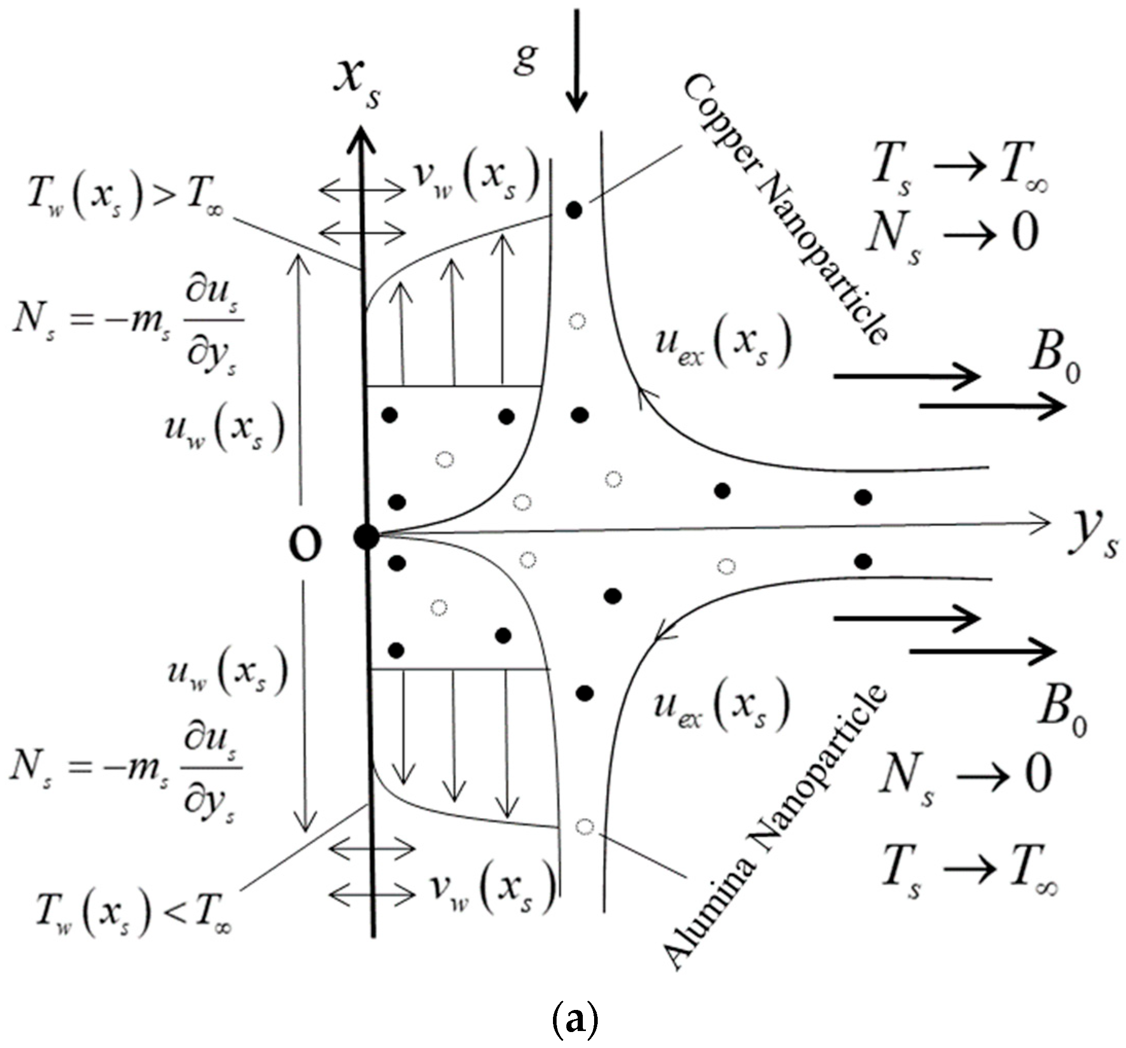
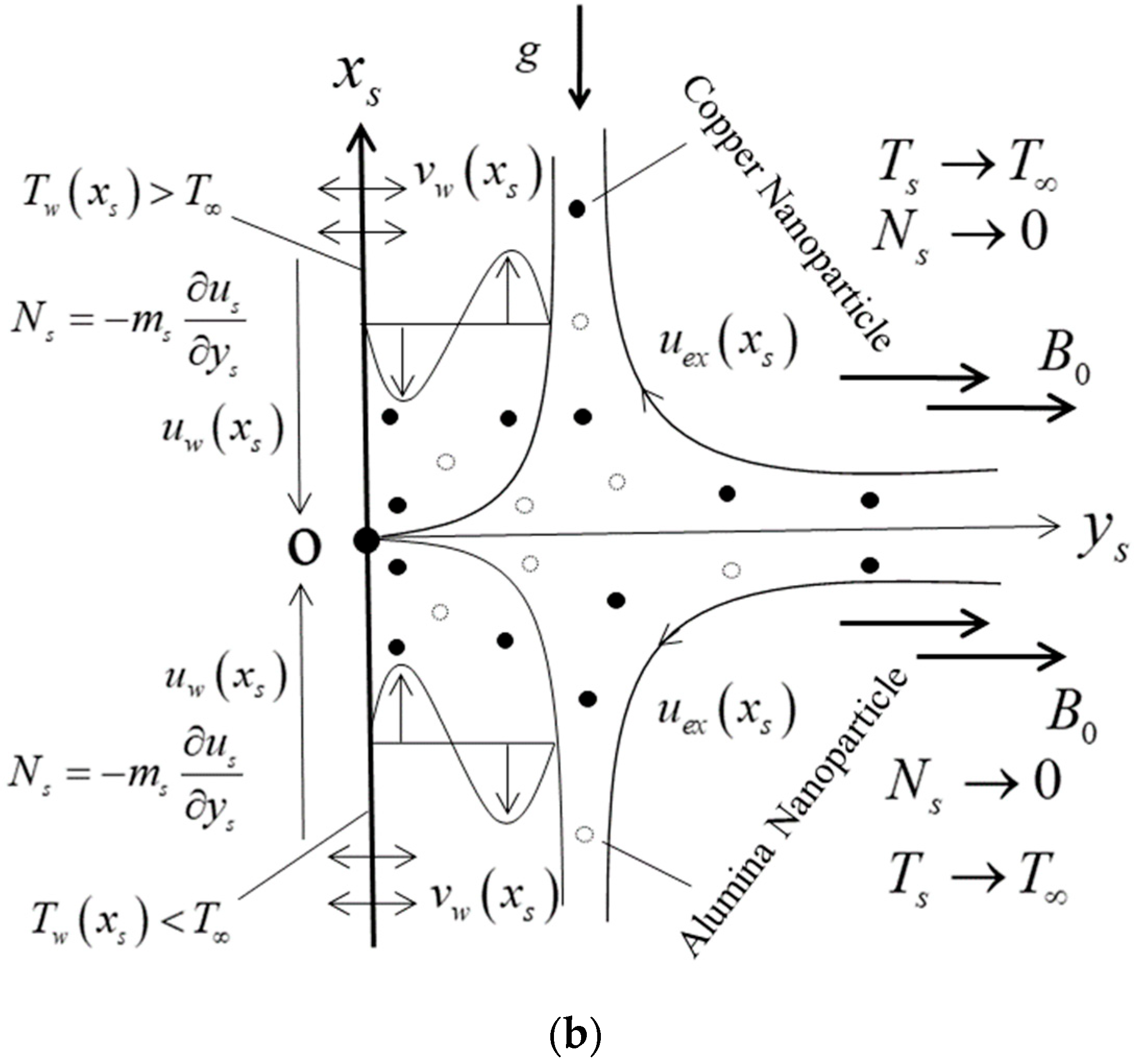
Let us consider the two-dimensional (2D) buoyancy or the mixed convective flow induced by micropolar hybrid nanofluids close to the SP over a porous vertical stretched or shrinking sheet.
Figure 1 shows this flow configuration along with the wall surface velocity
and free stream velocity
, in which
and
indicate the Cartesian coordinates appraised along the stretched or contracted sheet and orthogonal to it, respectively. The hybrid nanofluid is made up of a water-based fluid and two different kinds of nanoparticles, copper (Cu) and alumina (Al
2O
3). Additionally, it is conceivable that the configuration of the fluid flow was also affected by the combined effects of thermal radiation and an irregular heat sink/source term. Another presumption is that the wall variable temperature and constant far-field temperature are signified by
and
, respectively. The magnetic field measured to the sheet is assumed to have a constant strength
. Additionally, it is anticipated that the nanoparticles and water-based fluid would not slip and would be in thermal equilibrium. The single-phase method used in this hybrid nanofluid model assumes that the nanoparticles are homogenous in size and shape, and they do not interact with the surrounding fluid (see Sheremet et al. [
36], Pang et al. [
37], and Ebrahimi et al. [
38]). This statement supports the adoption of the single-phase model in this study since it is practically applicable when the base fluid can be effectively disseminated and is thought to behave as a single fluid.
These hypotheses, along with the Boussinesq and boundary layer approximations, are taken into consideration while presenting the main governed equations in terms of PDEs as follows [
23,
24,
25]:
when the boundary conditions (BCs) are
where
and
indicate the elements of velocity in the posited
and
axes, respectively,
the temperature,
the acceleration caused by gravity,
the microrotation,
the vortex viscosity, and
the micro-inertia density,
signifies the wall mass transpiration velocity with
the case of blowing and
the case of mass suction. According to these Refs. [
39,
40,
41],
is steady with the given closed interval
. The limiting case condition
is enforced in the case of strong concentration where the penetrating particles close to the contracted or stretched sheet do not swivel. The strong concentration or the high level of focus and the slip-free situation
in the specified limiting instance are similarly matched. The microstructure particles have a negligibly small impact close to a sheet that is stretched or contracted, and this behavior is documented for the case when
. Particularly,
indicates the weak concentration while the turbulent BLF is produced owing to the suitable case for
.
Furthermore,
represents the electrical conductivity of the hybrid nanofluid,
denotes the absolute viscosity of the hybrid nanofluid,
represents the thermal expansion coefficient (TEC) of the hybrid nanofluid,
represents the density of the hybrid nanofluid,
represents the thermal conductivity (TCN) of the hybrid nanofluid, and
represents the specific heat capacitance of the hybrid nanofluid. The relations of these thermo-physical hybrid nanofluid symbols in the expression form are as follows (see Oztop and Abu-Nada [
42]):
where;
and
and
Here,
portrays the nanoparticles volume fraction. Particularly,
represents the solid copper nanoparticles,
represents the alumina nanoparticles, and
represents the based (water) fluid. In all the computations, we have represented the nanoparticles
and
by
and
, respectively. Moreover,
,
,
,
,
and
denotes the density, absolute viscosity, TCN, specific heat capacitance, TEC, and electrical conductivity of the based (water) fluid, respectively. Also, the physical data of the carrier-regular fluid and the binary nanoparticles are shown in
Table 1. The numerical calculations for this analysis will benefit from these thermophysical features.
Moreover, the final term
in the RHS of Equation (4) demonstrates the part of irregular heat source/sink, which can be established as [
43]:
Here,
denotes the exponential decay space coefficients, and
denotes the temperature-dependent heat sink/source. Besides, the situation of a heat absorption or source refers to the positive value of
and
, whereas the behavior of a heat generation or sink corresponds to the negative value of
and
. In addition, the second last term
in the RHS of Equation (4), called the radiative heat flux, is mathematically demarcated via the Rosseland approximation as [
32]:
where the letter
indicates the Stefan Boltzmann constant and the letter
denotes the mean absorption coefficient. By exercising the Taylor series, the fourth power of
expanded around a unique point
and ignoring the higher-order power, one obtains the form as:
Hence, by substituting Equations (12)–(14) into Equation (4), the following equation is obtained:
Equations (2), (3) and (15), along with BCs (5), need to change into similarity forms by executing the following terms
Here, the constants are mentioned by and while denotes the mass transpiration parameter, where indicates the suction, indicates the injection, and indicates the impermeable surface of the sheet. Meanwhile, signifies the uniform reference temperature, with indicating the assisting flow (heated surface) while signifies the opposing flow (cooled surface).
To comfort further the scrutiny of the given model, the following similarity letters or variables are given
where
represents the carrier-based fluid (kinematic viscosity). Additionally, the elements of the posited velocity in relation to the “stream function” are defined in the following usual way as
so that the continuity Equation (1) is true. Also, the components of velocity after utilizing Equation (18) are sealed in the following form:
Putting Equation (17) into governed Equations (2), (3) and (15), we get the following requisite posited ODEs:
where the primes denote the derivative w.r.t to
(the pseudo-similarity variable). Let
In Equations (20)–(22), indicates the material parameter, indicates the micro-inertia factor, indicates the magnetic factor, indicates the radiation factor, and indicates the buoyancy or mixed convective factor, where and identify as the local Reynolds number and the local Grashof number, respectively.
The BCs (5) can be rewritten in the dimensionless form and are
In Equation (23), is the stretched or contracted parameter where is for stretching, is for shrinking, and is for static.
2.1. The Engineering Quantities of Interest
The behaviors of the thermo-micropolar HN flow in the current model are described using the surface shear stress, gradient of microrotation, and rate of heat transfer.
2.1.1. The Shear Stress Coefficient (SSC)
The SSC is demarcated as
where
is the wall SS for the micropolar HN. Substituting Equation (17) into Equation (24), the reduced SSC may be expressed as
2.1.2. The Couple-Stress Coefficient (CSC)
Here, the wall CS of the micropolar HN is signified by
in which
corresponds to the spin gradient of the HN. The following dimensionless form of the CSC is obtained by using Equation (17) in the aforementioned equation.
2.1.3. The Heat Transfer Rate (HTR)
The HTR at the surface is demarcated as
where
specifies the heat flux at the wall surface for the micropolar HN. Finally, using the similarity variables in Equation (28), one obtains the following dimensionless form of the HTR
5. Analysis of Results
The thermo-micropolar (water/Cu-Al
2O
3) hybrid nanofluid and heat transfer flow examination comprised several distinct distinguished parameters which are namely and symbolically denoted as
for the magnetic factor,
for the material factor,
for the micro-inertia factor,
for the radiation factor,
for the mass suction/injection factor,
for the stretched/shrinked factor,
for the mixed convection or buoyancy factor, and
and
for the solid nanoparticles volume fraction. The physical impact of these numerous notable influential parameters on the shear stress coefficient, couple-stress coefficient, heat transfer, and temperature profile was presented tabularly in
Table 4,
Table 5 and
Table 6, but graphically illustrated in
Figure 2,
Figure 3,
Figure 4,
Figure 5,
Figure 6,
Figure 7,
Figure 8,
Figure 9,
Figure 10,
Figure 11,
Figure 12,
Figure 13,
Figure 14,
Figure 15 and
Figure 16, respectively. However, the eigenvalue
for the several/sundry values of
is established in
Figure 17 while the streamlines are presented in
Figure 18 and
Figure 19. For the computation purpose, we have executed the following ranges for the parameters such as
,
,
,
,
,
,
,
,
, and
. Furthermore, the first branch solution (FBS) and second branch solution (SBS) are highlighted by the complete filled solid and dashed black lines, respectively, while the black solid balls denoted the critical or bifurcation points.
Table 4 and
Table 5 demonstrate the quantitative values of the shear stress coefficient (SSC) and couple-stress coefficient (CSC) for the FBS as well as the SBS due to the distinct values of the solid nanoparticles’ volume fraction, material parameter, magnetic parameter, mass suction parameter, and the micro-inertia parameter, respectively, when
,
,
,
,
, and
. It was observed that the shear stress coefficient for the FBS escalated and decelerated for the SBS with the superior impact of
,
,
, and
while contrary behavior was seen in two outcome branches for the larger values of
(see
Table 4). Generally, the higher magnetic impression creates the strong Lorentz force by which the velocity profile declines. As a result, the speed/motion of the fluid (or velocity profile) has an inverse relation with the skin friction coefficient. According to the basic rule of physics, if the velocity of the fluid shrinks with strong influences of the magnetic parameter, as a response the shear stress coefficient uplifts. On the other hand, the output values pattern/tendency of the CSC for the FBS remains the same as (the SSC) with the larger impacts of
and
while it declines for the SBS, and also magnitude-wise, is augmented. Furthermore, the CSC diminished for both FB and SB outcomes with augmentation in the values of
and
as depicted in
Table 5. Generally, the absolute/dynamic viscosity of the fluid reduces due to the higher influences of the material parameter, hence, the CSC lessens.
Table 6 depicts the values of the heat transfer rate (HTR) for the FB as well as the SB solution with deviation in the larger selected values of
,
,
,
, and
when
,
,
,
,
,
, and
. The results reveal that the values of the heat transfer enrich for both branches owing to the mounting values of the radiation parameter,
and
. Also, the heat transfer inclines for the SBS and decays for the FBS in magnitude with larger impressions of the heat source factor (
) while the pattern of the output values were reversed in both branches for the superior impacts of the heat sink factor (
).
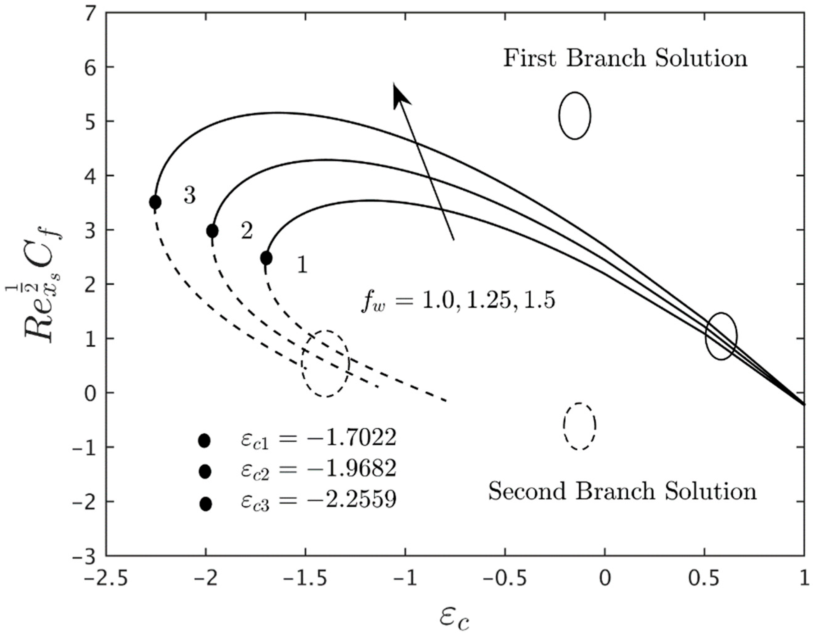
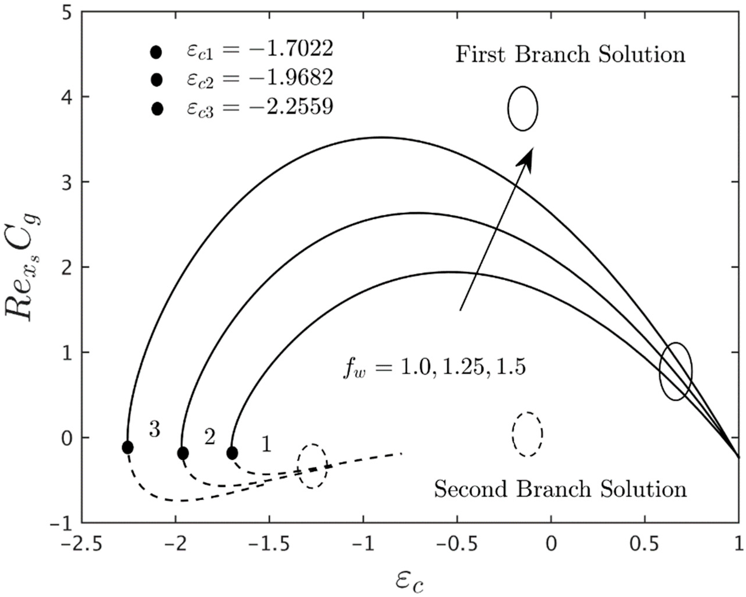
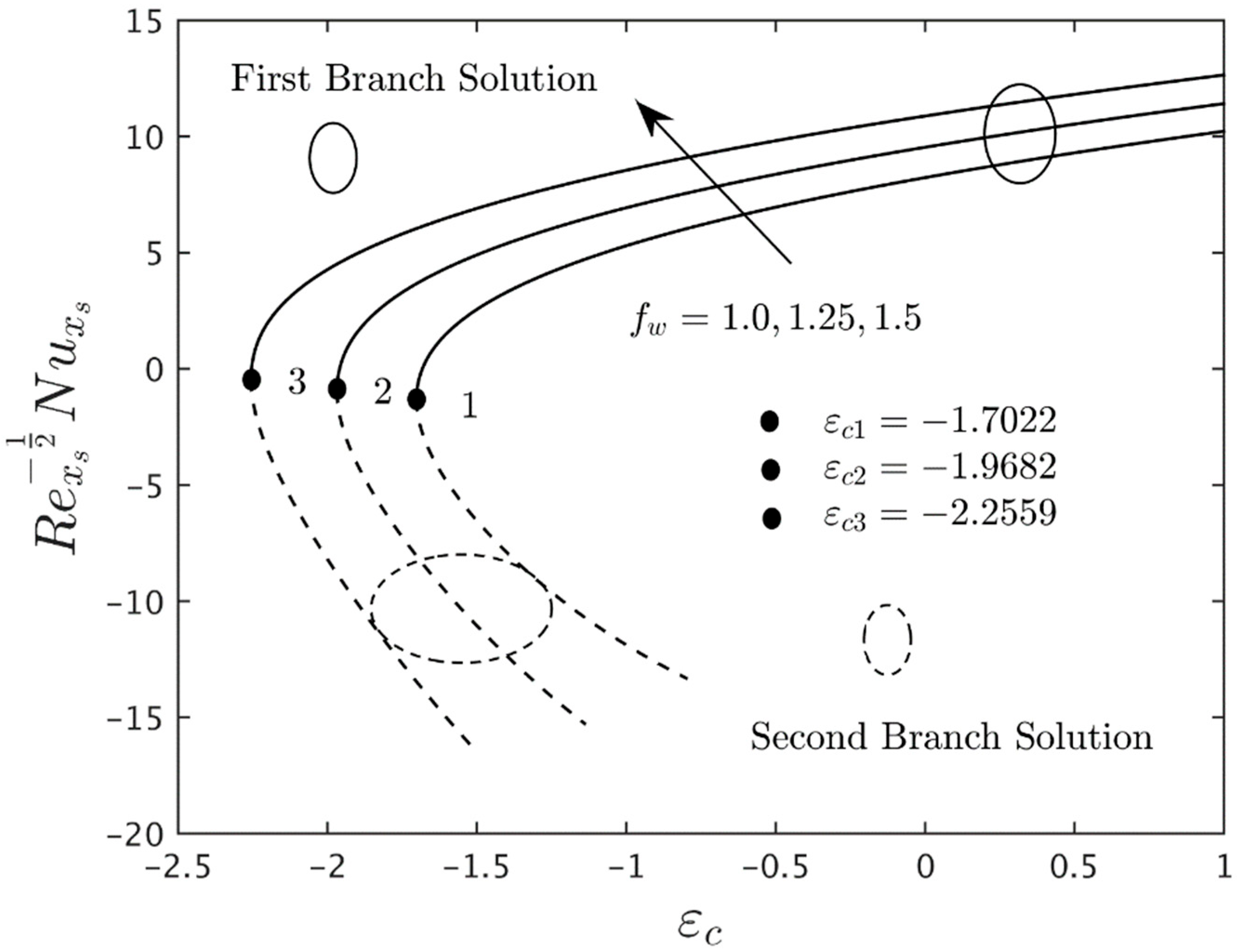
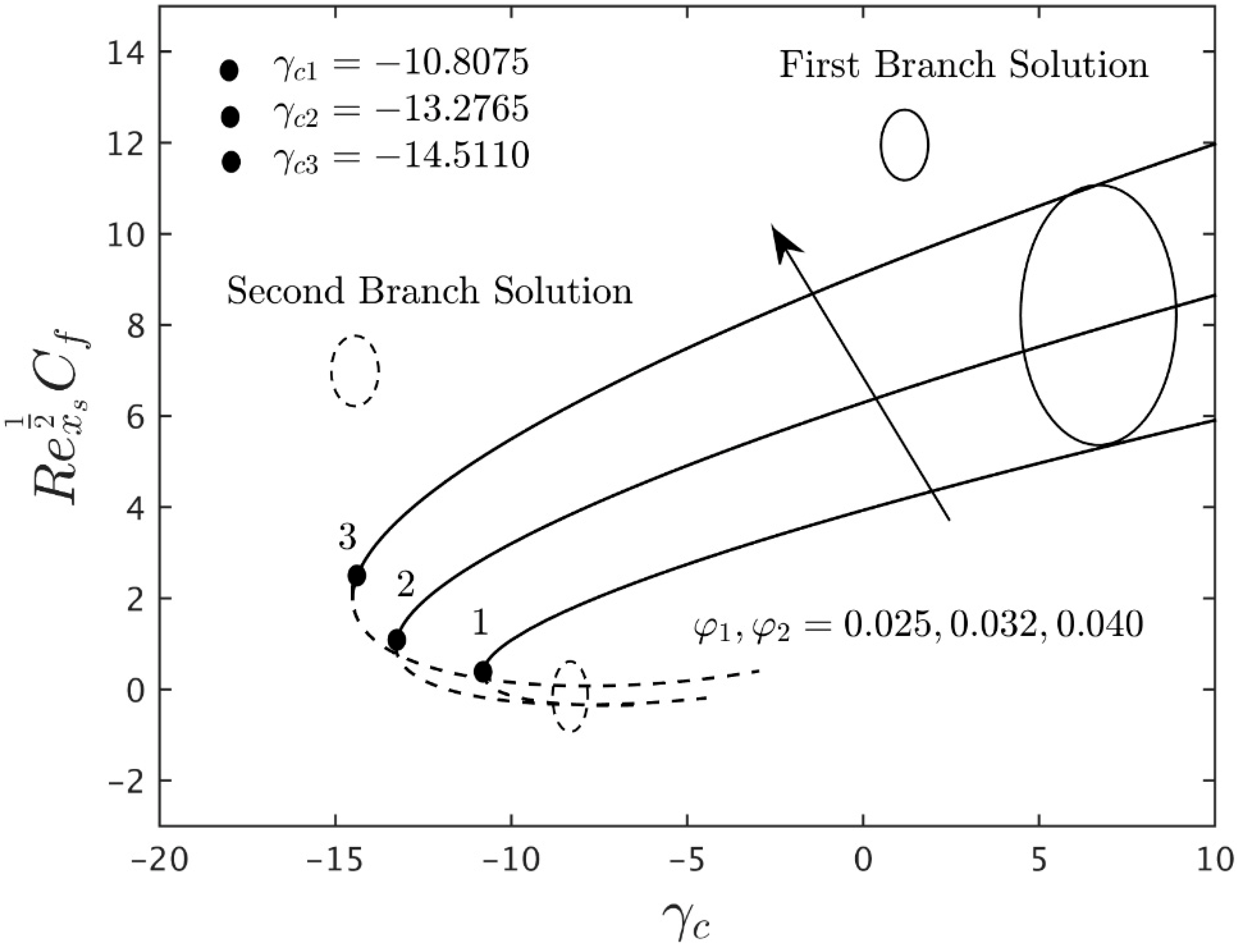
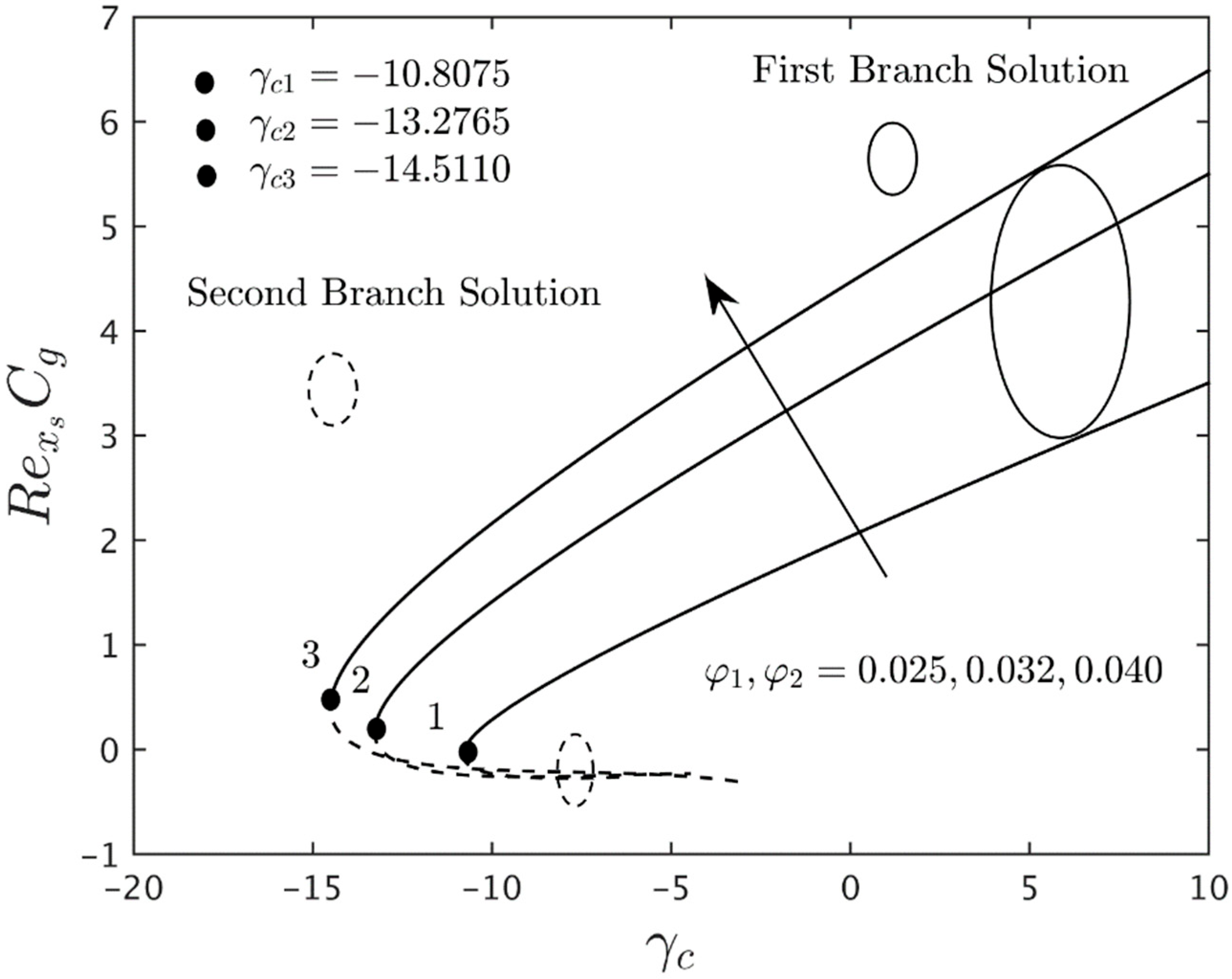
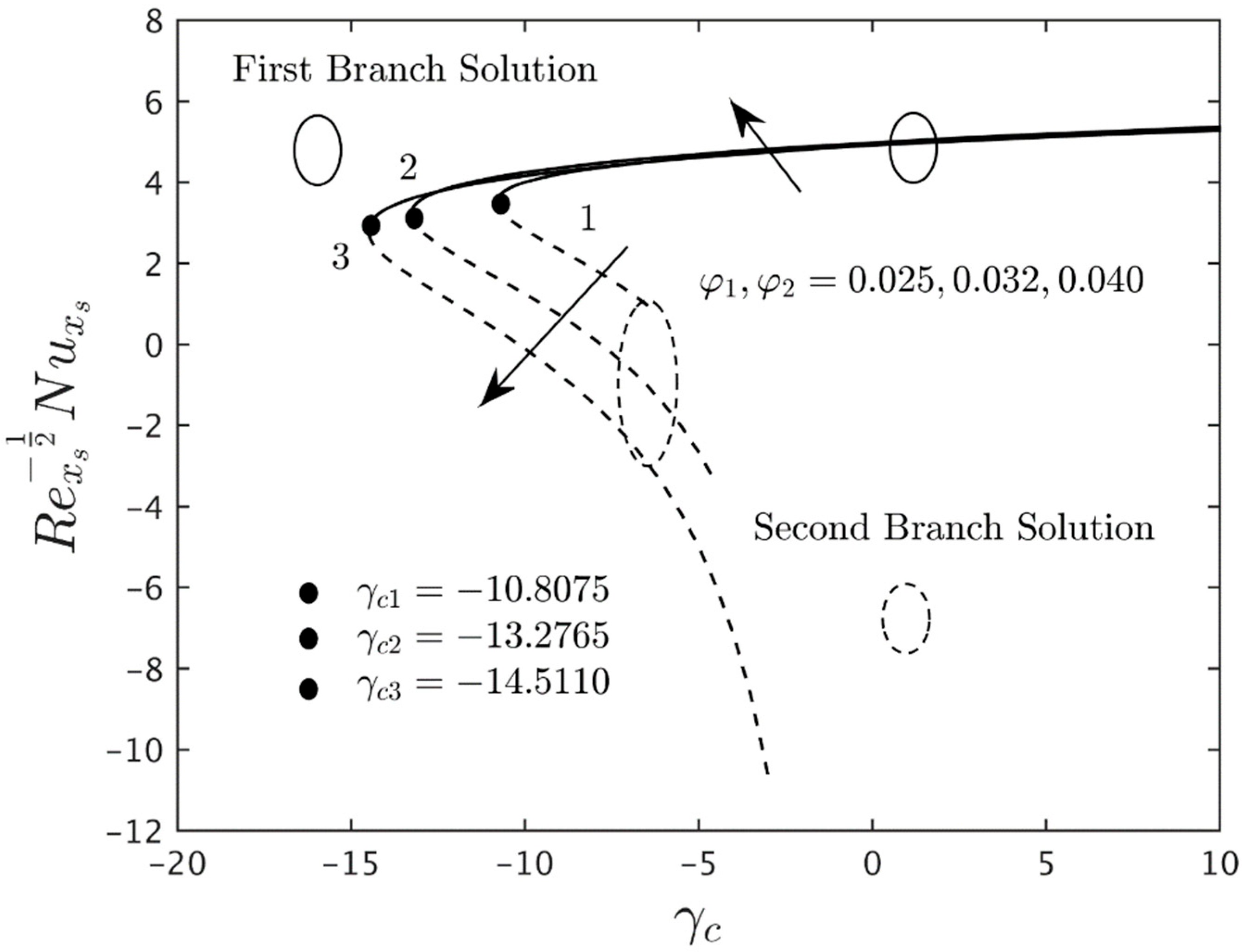
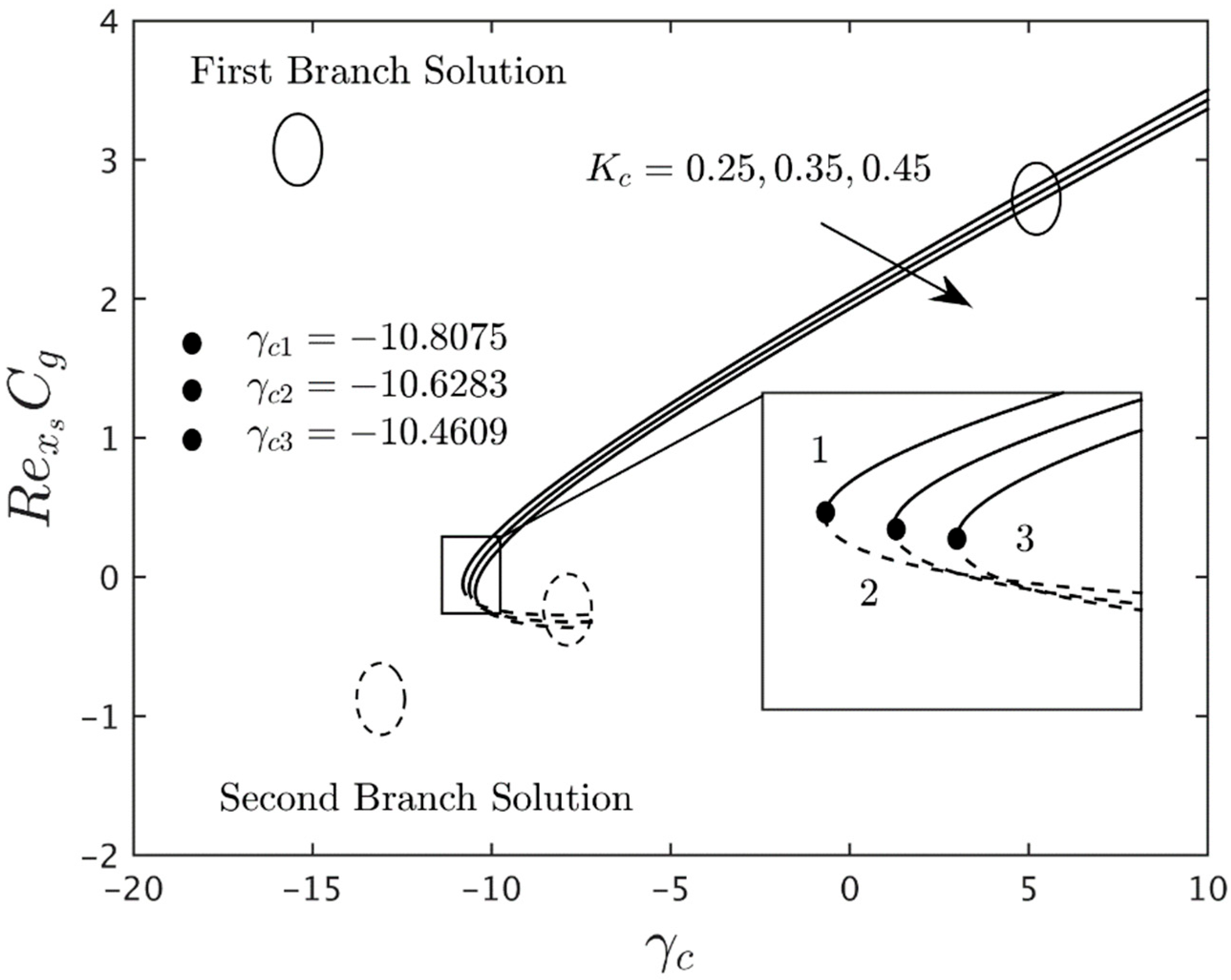
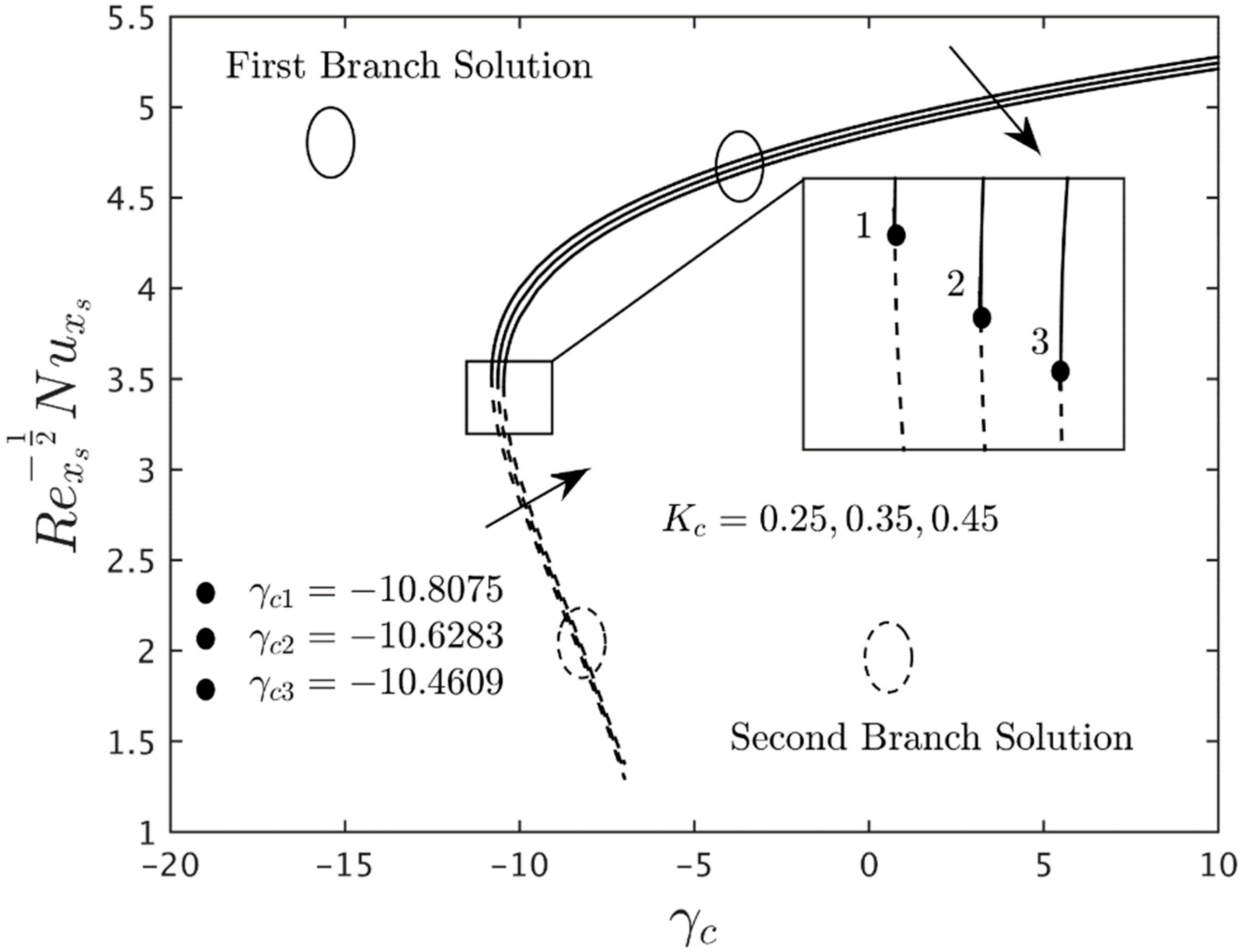
Figure 2,
Figure 3,
Figure 4,
Figure 5,
Figure 6 and
Figure 7 portray the variation of the reduced SSC (shear stress coefficient), the gradient of micro-rotation or CSC, and the heat transfer of the (water/Cu-Al
2O
3) hybrid nanofluid for the several values of
and
. It was found that multiple or double solutions (FB and SB results) happened for Equations (20)–(22) subject to the BCs (23) in the region of
, in which
represents the bifurcation value of
. Note that a unique solution exists for
, while no solutions exist when
. Additionally, from these graphs, it is clear that the output values of
upsurge as the requisite parameters
and
upsurge, indicating that these factors/parameters expand the range in which dual/double solutions can occur. Further evidence supports the idea that the inclusion of hybrid nanoparticles, the suction effect, the magnetic field, and the stretching sheet could slow the boundary layer separation (BLS), but the presence of the material parameter and the shrinking sheet could speed up the BLS. Also, for the FBS, the values of the HTR and CSC are consistently positive owing to the HT from the precise hot surface of the stretched/contracted sheet to the requisite cold fluid. The opposite pattern is noticed in the phenomenon of the SBS, i.e., the heat transfer rate and the couple stress coefficient become unavailable as
and
.
The impression of the mass suction parameter
on the SSC, CSC, and HTR of the (water/Cu-Al
2O
3) hybrid nanofluid for the FB and SB solutions is presented in
Figure 2,
Figure 3 and
Figure 4, respectively. The outcomes display that the gradients (SSC, CSC, and HTR) boosted up for the FBS due to the higher values of
while it declines for the branch of second solutions. In addition, it is noticeable that the SSC values of the FBS are slightly higher and better than the values of CSC with higher impacts of the mass suction parameter as seen graphically in
Figure 2 and
Figure 3. This behavior is due to the fact that the influence of the mass suction at the surface boundary of the stretched/shrinked surface slows down the hybrid nanofluid motion and escalates the shear stress and couple-stress coefficients at the surface of the vertical sheet. On the other hand, the rate of heat transmission developed as the magnitude of the mass transpiration parameter was boosted (see
Figure 4). According to this fact, the thermal boundary layer thickness decelerates with larger impacts of the mass suction parameter, and as a response, the temperature distribution gradient of the sheet uplifts.
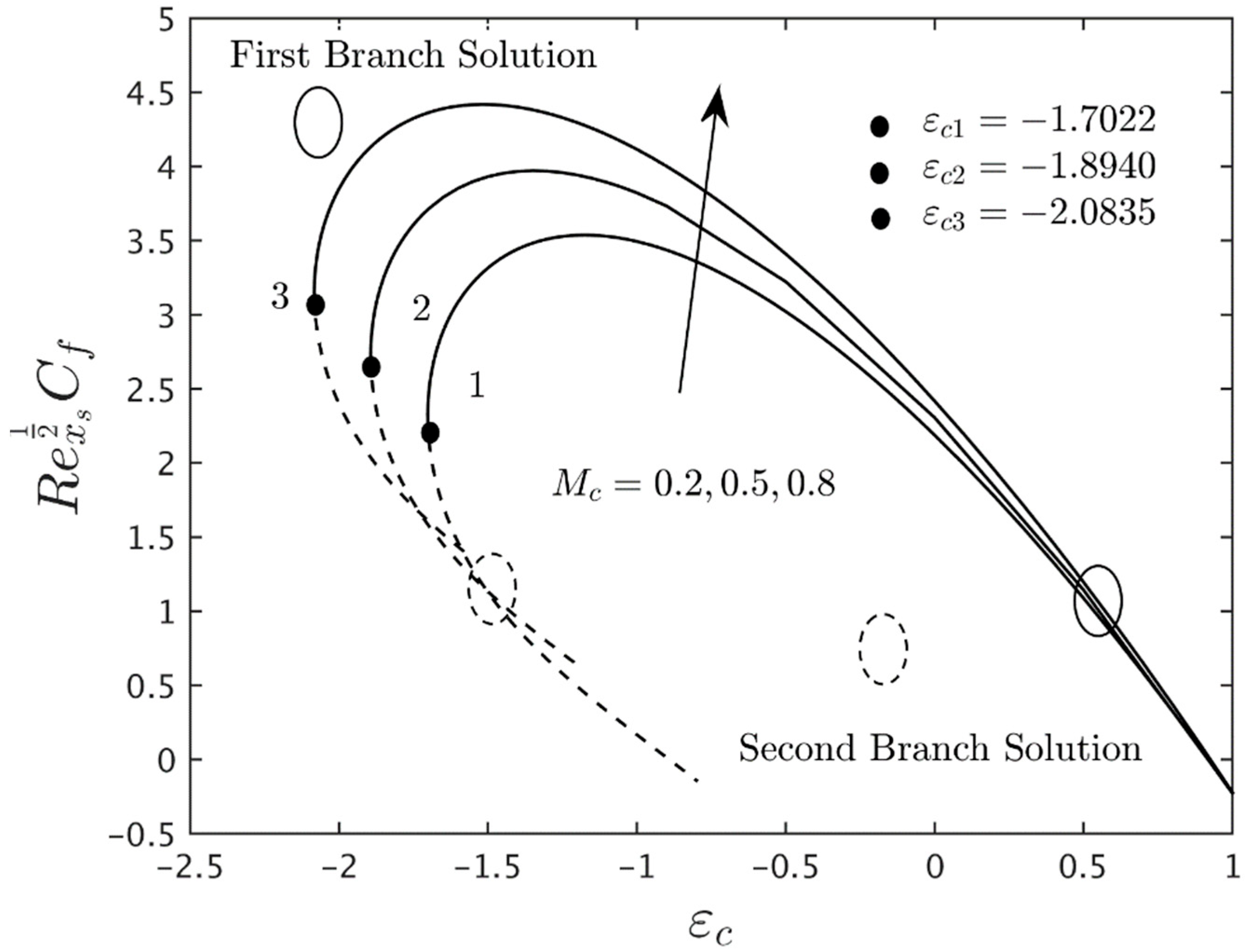
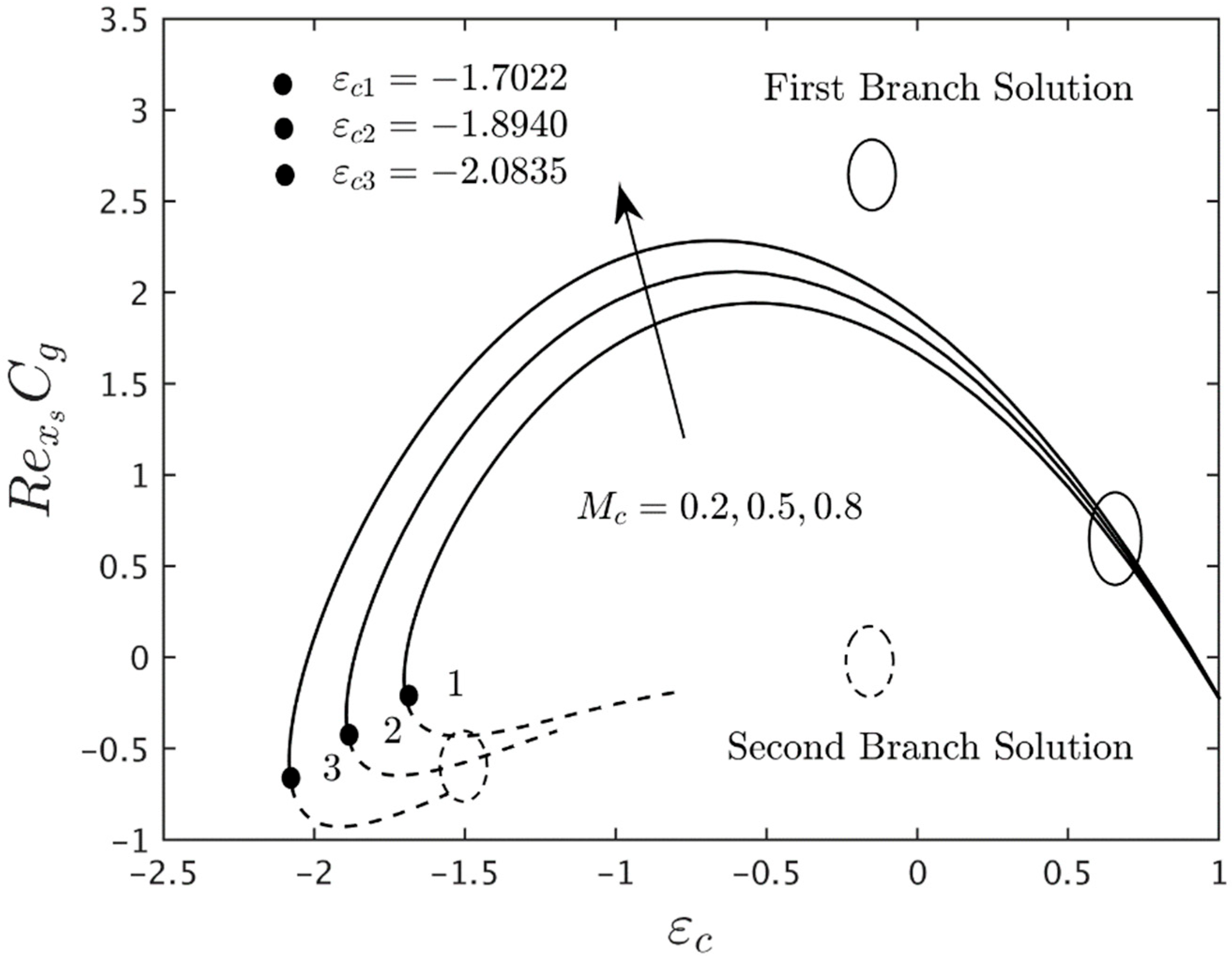
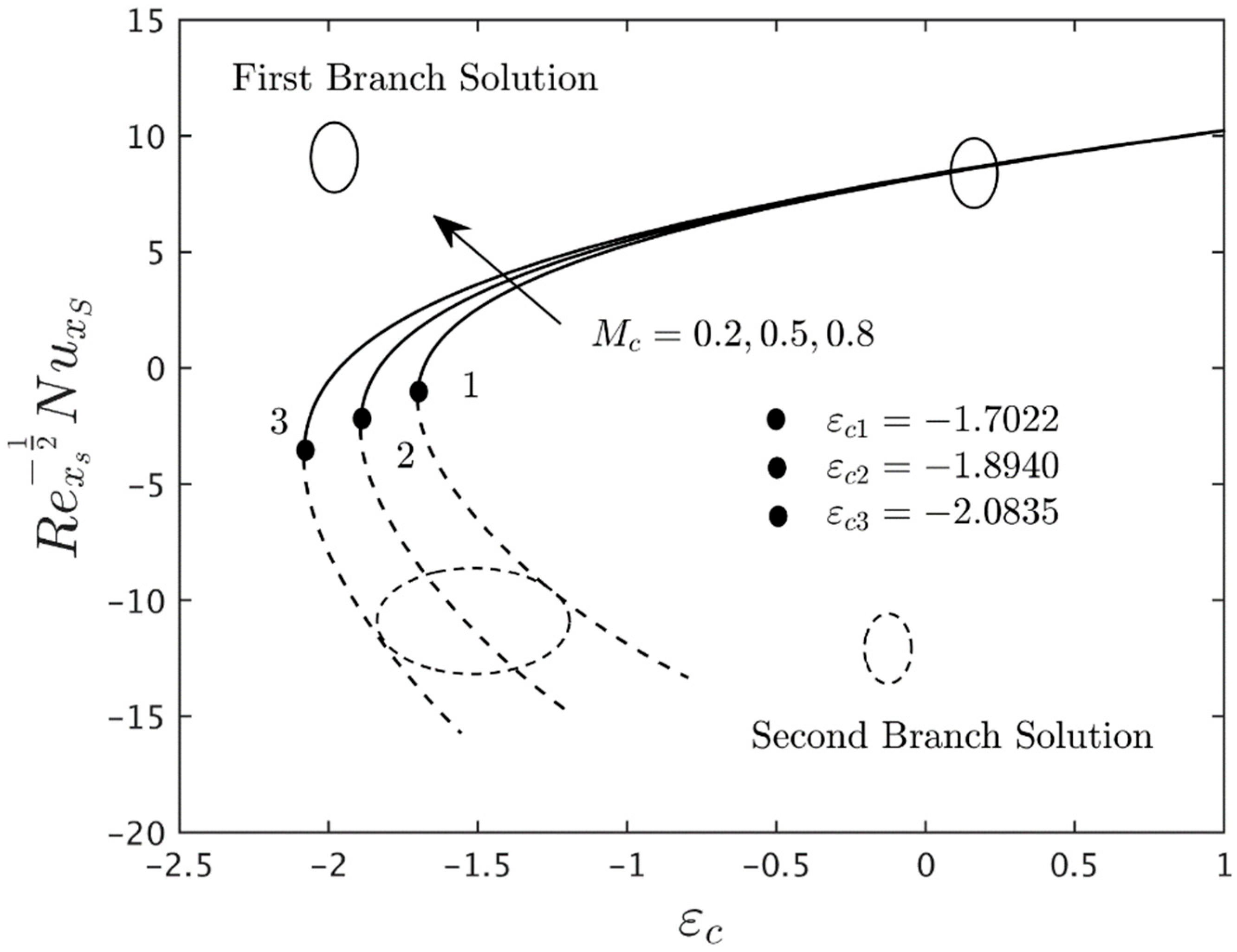
Figure 5,
Figure 6 and
Figure 7 illustrate the impacts of the magnetic parameter
on the SSC, CSC, and HTR of the (water/Cu-Al
2O
3) hybrid nanofluid for the FB and SB solutions, respectively. In these graphs, it is initiated that the CSC and HTR improve in the FBS but decay in the SBS owing to the larger impacts of
while the SSC behaves increasingly for the FB solutions and a monotonic kind of behavior or a changeable behavior was followed in the same branch, moving away from the critical values for the larger effects of the magnetic field. Physically, by enlarging the values of the magnetic parameter, a force is produced which slows down the motion of fluid along the stretching/shrinking sheet and increases the convection of thermal energy by boosting the interactivity of the fluid particles which is known as the Lorentz force. According to this force, the speed of the hybrid nanoparticles of the fluid slows down. As a result, the shear stress and couple-stress coefficients are enlarged. Additionally, the gap among the curves for the FB is compared to the SB solutions as seen in
Figure 5 and
Figure 6, and vice versa, for the heat transfer rate as graphically depicted in
Figure 7. Furthermore, when the effects of magnetic field strength grow, the rate of heat transmission increases. This tendency results from the decreasing thermal boundary layer thickness caused by a growing magnetic field, which causes an intensification in the posited temperature gradient at the vertical sheet’s surface.
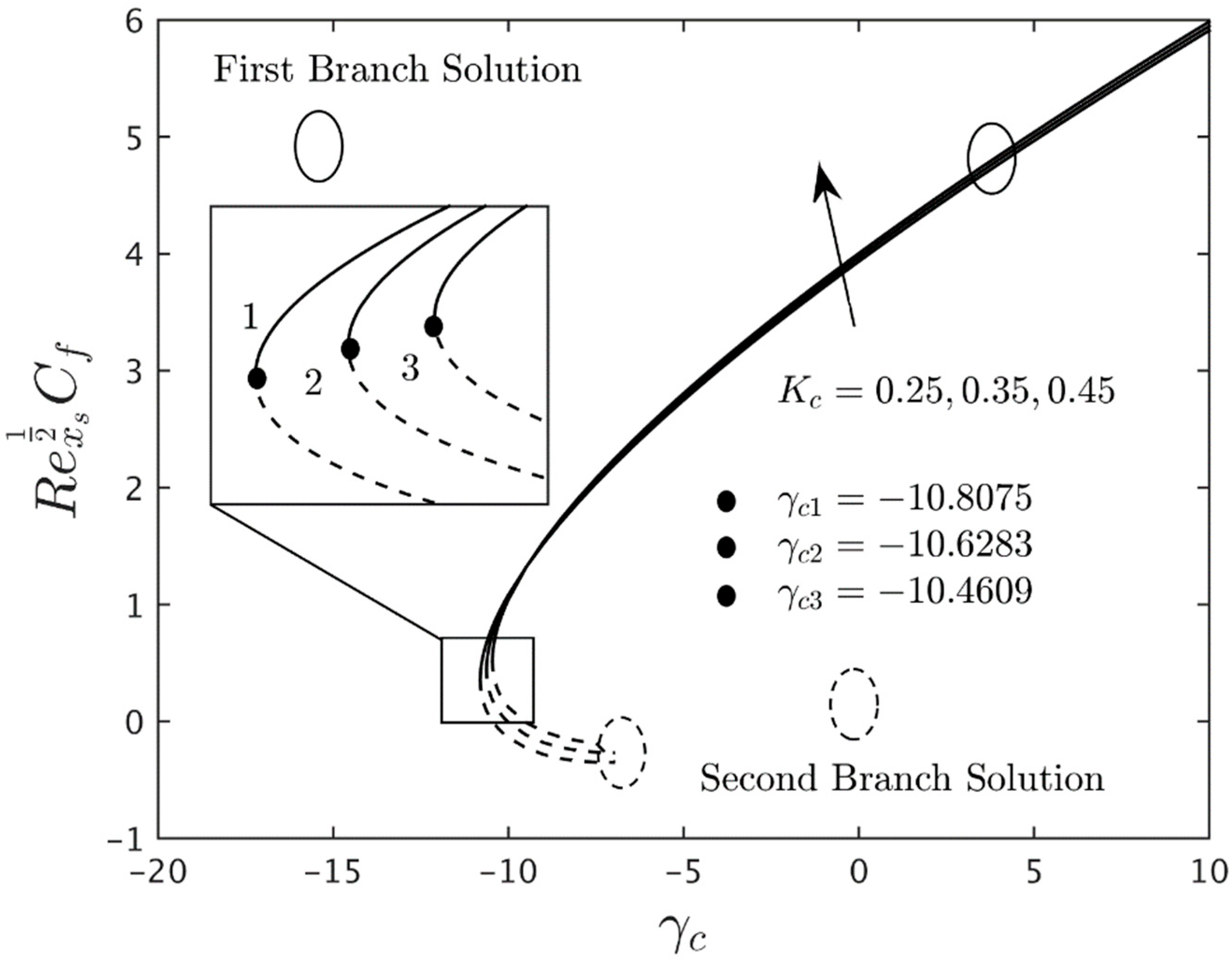
The impacts of the solid nanoparticles volume fraction
and
on the shear stress coefficient (SSC), couple stress coefficient (CSC), and heat transfer rate for the double branch (FB and SB) solutions versus the mixed convection parameter
are described in
Figure 8,
Figure 9 and
Figure 10, respectively. These figures show that the heat transfer rate, shear stress, and couple-stress coefficients enrich for the first branch solutions due to the larger values of
and
. Alternatively, the HTR declines for the SBS with higher impacts of
and
while the shear stress and couple-stress coefficients behave similarly to the FBS. Generally, there is a direct correlation between the volume percentage of nanoparticles and the temperature profiles. By increasing the volume percentage of nanoparticles, the thermal conductivity increases, which results in a monotonic development of the thermal boundary layer thickness and the temperature distributions. Due to this reason, the thermal conductivity rises as the volume percentage of nanomaterials increases, resulting in the thermal BLF and the HTR of the sheet. Furthermore, it is revealed that the two branches (FB and SB) solution is possible in the region when
, in which
is the critical/bifurcation value of
. Moreover, the outcome is not possible for the posited range
, while a unique or solo solution is initiated at the specific bifurcation point
. Besides, the magnitude of the gradients (SSC, CSC, and HTR) uplifts with the rise of the solid nanoparticles volume fraction
and
. In other words, the absolute output numbers of
are revealed to be superior for larger values of the solid nanoparticles volume fraction
and
(see
Figure 8,
Figure 9 and
Figure 10). Hence, the impact of
and
upsurges the region of the mixed convection or buoyancy parameter for which the outcome is possible to exist. These plots additionally reveal that the bigger value of the hybrid nanoparticles slows down the BLS.
Figure 11,
Figure 12 and
Figure 13 show the variation of the respective SSC, CSC, and HTR of the (water/Cu-Al
2O
3) hybrid nanofluid for the FB and SB solutions due to larger values of the material parameter
. Notably, it is evident from the
Figure 11 and
Figure 12 that the shear stress initially declines and then upsurges for the FBS with a higher impact of material parameters, but the couple shear stress continuously decreases for the FBS. Whereas, for the branch of second solutions, the gradient of micro-rotation escalates due to larger values of
, while shear stress decelerates and behaves vice versa. On the other hand, the heat transfer decreases and increases for the branch of the first and second solutions, respectively, owing to the superior hammering of the parameter
(see
Figure 13). In all three graphs, the gap was slightly lesser in both solution branches, therefore, we have to zoom in on the specific part where both solutions can meet or merge at a single point, called a bifurcation point
. The bifurcation values for the distinct choices of
are shown by the small solid black balls and also numerally highlighted in the suggested plots. Additionally, the absolute values of
are smaller for the superior values of
. In this regard, the pattern of the outcomes indicates that the larger values of the material parameter speed up the level of the separation of the boundary layer.
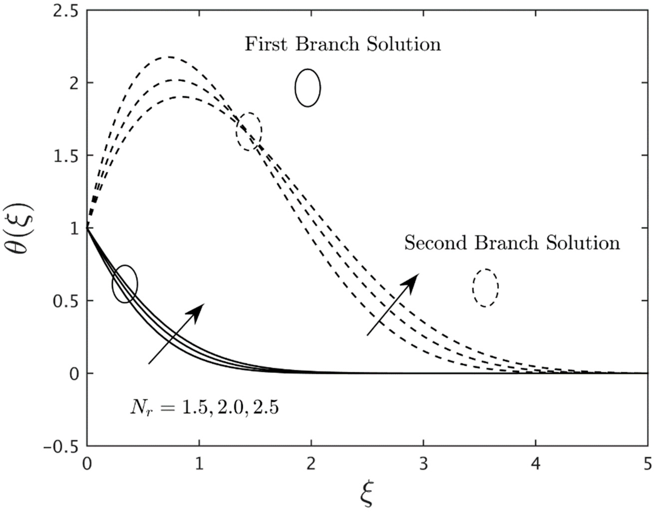
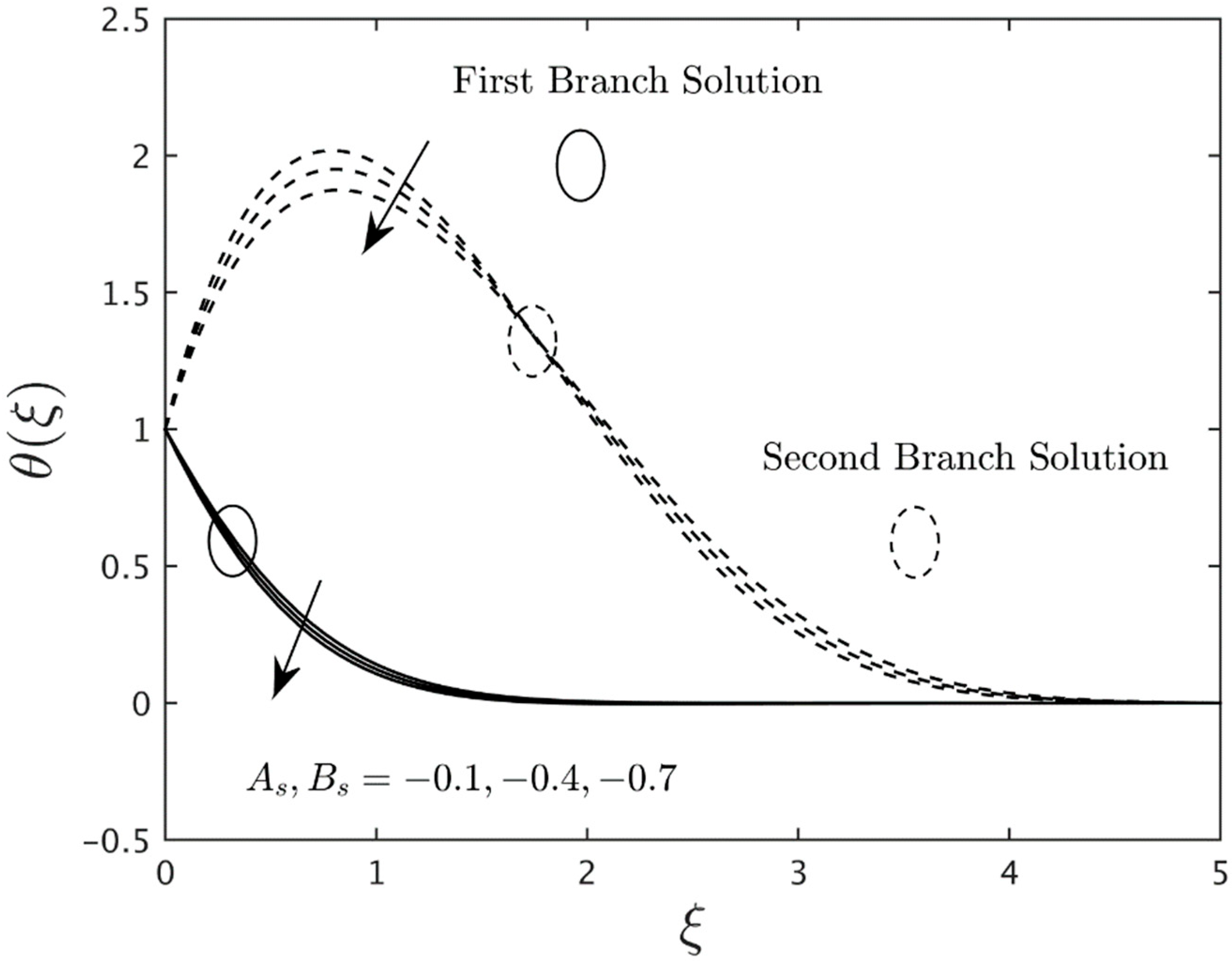
The effects of the radiation parameter
on the temperature distribution profiles of the (water/Cu-Al
2O
3) hybrid nanofluid for both branches of solutions is graphically exemplified in
Figure 14. From the graph, it is seen that both solution branches and the thickness of the TTBL boosted up as the value of the
was augmented. Moreover, the double branch (FB and SB) solutions asymptotically hold the boundary Conditions (23). Also, the gap in both solution curves is reasonable/understandable for the higher impacts of the radiation parameter. Physically, the thermal conductivity is improved by bigger values of the radiation parameter, which can lead to an increase in temperature distribution profiles as well as in the thickness of the thermal boundary layer.
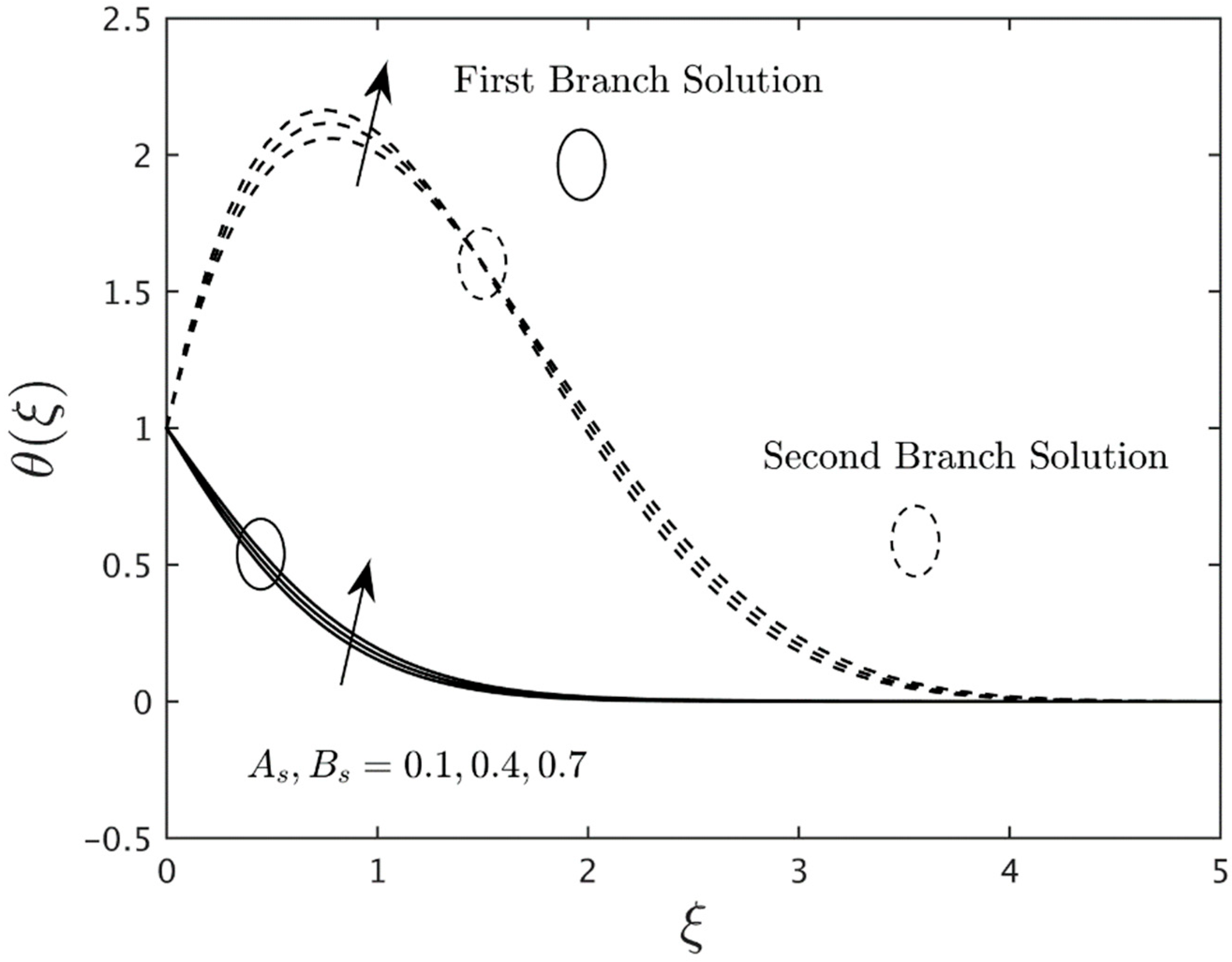
Figure 15 and
Figure 16 designate the significance of the internal heat source factor
and heat sink constraint
on the temperature field curves of the (water/Cu-Al
2O
3) hybrid nanoparticles, respectively. In both graphs, the results were constructed/prepared for the branch of the first and second solutions. In addition, the outcome of both plots demonstrates that the profile of the temperature and the TTBL augment with the superior impacts of the internal heat source factor for the FBS as well as for the SBS, while it is reducing continuously with the internal heat sink factor. Generally, the reason this happens is because the heat source factor causes the system to absorb more energy as a result of heat, and, as a response, the temperature enriches (see
Figure 15). On the other hand (see
Figure 16), the system did not receive a better level of heat (in the form of energy) owing to the requisite heat sink factor and, as a consequence, the temperature profile decelerated. Furthermore, the gap in both solution cases is looking similar to the rising value of the internal heat source/sink factors.
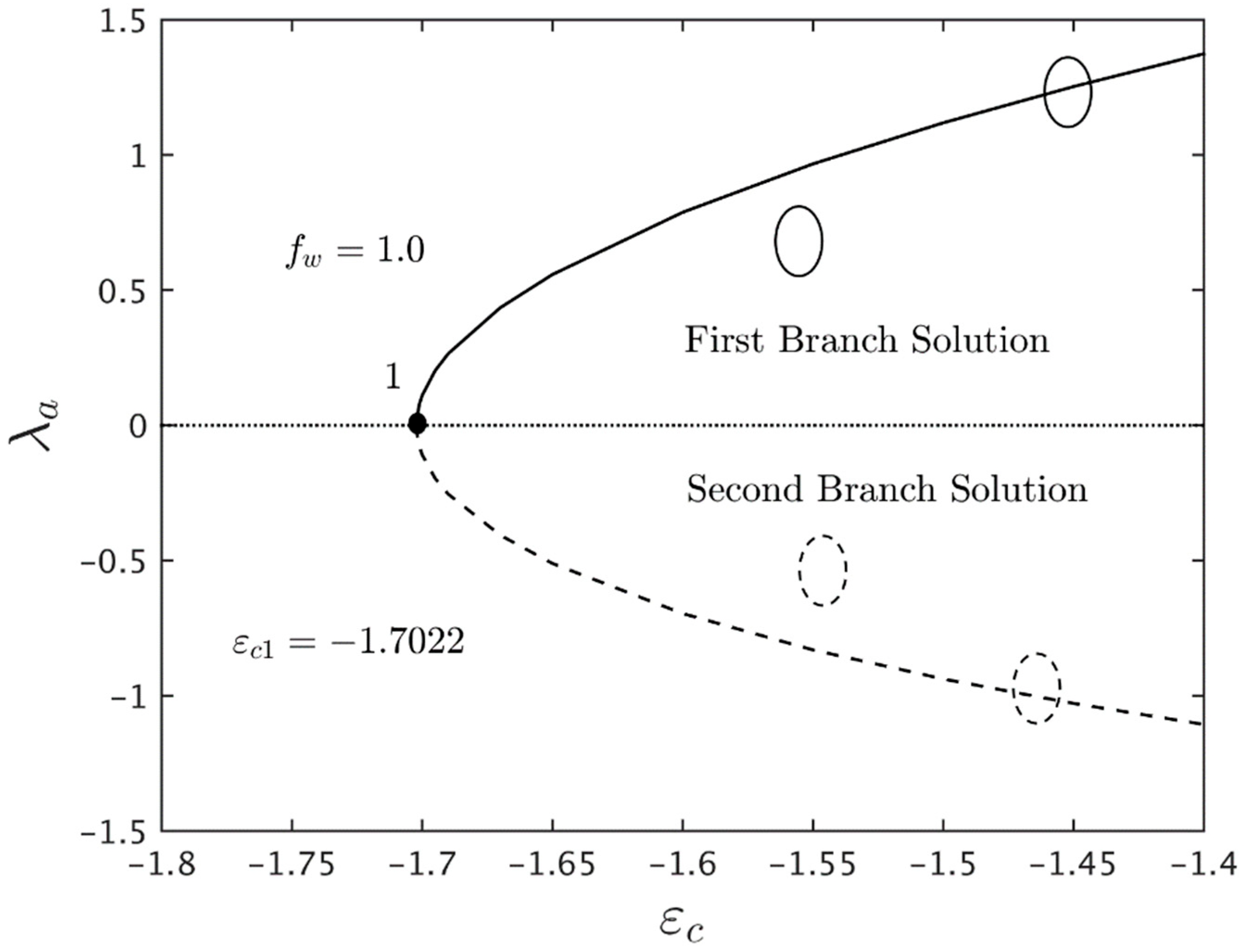
The temporal stability analysis was assumed to check the stability of the multiple or double-branch solutions. Thus, the smallest eigenvalue
was calculated by solving the linear eigenvalue Problems (39)–(42) using the built-in code working in MATLAB.
Figure 17 shows the minimum eigenvalue
against the posited parameter
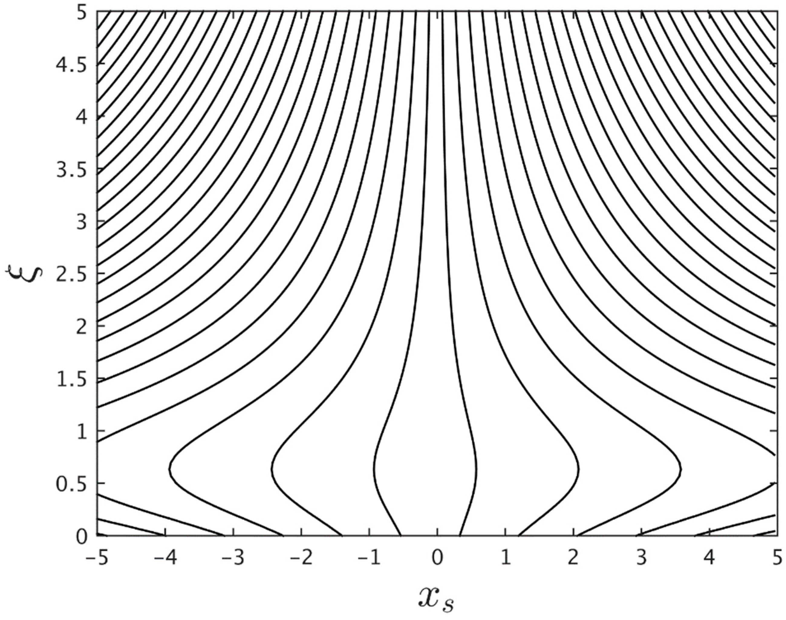
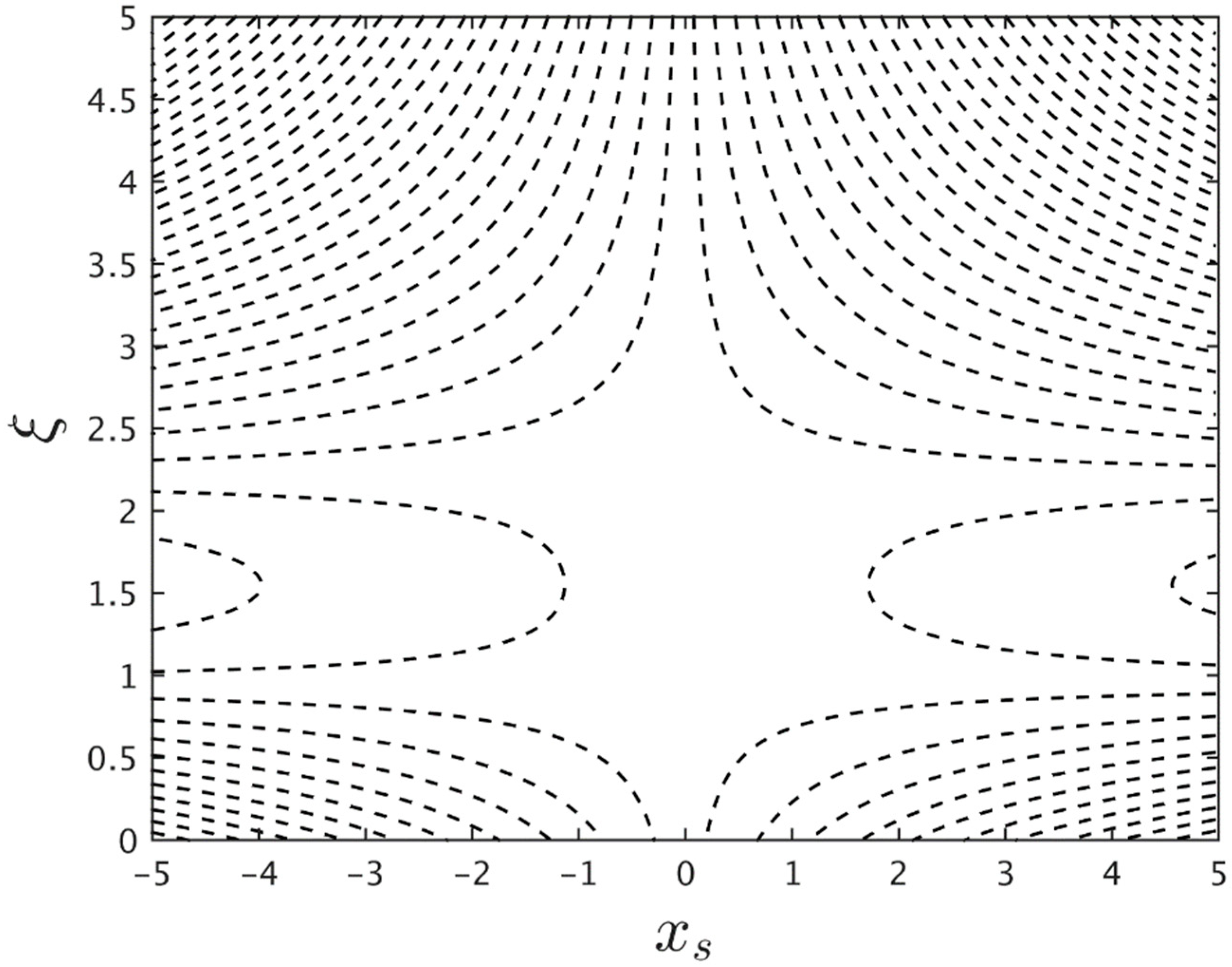
. The first branch solution is represented by the positive eigenvalue, whereas the second branch solution is represented by the negative eigenvalues. It may be determined that the first-branch solution is stable and substantially more practicable than the second-branch solution, which is unstable and physically not acceptable. Furthermore, the streamlines pattern for the upper and lower branch solutions are represented in
Figure 18 and
Figure 19 when
. Outcomes show that for the branch of the top solution, the streamline pattern is simple curves and symmetric in the corresponding axial axis, however for the lower branch solution, the streamlines pattern is ambiguously complex and divided the flow into double regions.

 ,
, 


