1. Introduction
Biotechnological processes are one of the fastest-developed strategic fields of science and practice, and have had a great advance in recent years. Due to their multidisciplinary nature and enormous capabilities, they have been applied by microbiologists, biochemists, molecular biologists, bioengineers, chemical engineers, food and pharmaceutical chemists, mathematicians, and a whole range of other scientists. These processes are known to be with complicated structure of organization and interdependent characteristics, which determine their non-linearity and non-stationary properties. Therefore, the mathematical modelling design, optimization, and high-quality control of the underlying processes are very complex, rather time consuming, and costly tasks. The modelling of a bioprocess is a very important process through which the radical principles of microbial synthesis can be discovered. The dynamics of a biotechnological process can be described by using a balance equation on how to apply the radical parameters of a process: Cell density, substrate concentration, profitable product, oxygen concentrations, temperature, pH, and time [
1].
Ethanol is the most important organic compound, which has a wide application in different industries: Food, perfumery-cosmetic, chemical, millwright, etc. In recent years, enormous attention has been paid to ethanol production for fuel. Ethanol production from renewable resources can improve energy security, reduce accumulation of carbon dioxide, and decrease urban air pollution. When blended with gasoline, “neat” ethanol reduces the release of smog-forming compounds. Thus, ethanol from lignocelluloses materials holds great promise as a new industry in the world, and has the potential for making a significant contribution to the solution of major energy, as well as environmental problems. Although ethanol production by fermentation of sugar has been studied for many years, there are several bottlenecks for the economical production of ethanol for fuel. One of them is ethanol inhibition, which is considered the principal factor restricting the fermentation rate, as well as the concentration of ethanol achieved during the production process [
2].
Multi-criteria decision making (MCDM) is a branch of operation research models and a well-known field of decision making. There are four quite distinct families of methods: (i) The outranking; (ii) the value and utility theory-based methods; (iii) the multiple objective programming; and (iv) a group of decision and negotiation theory-based methods. The main objective of MCDM is to select the alternative that has the highest score according to the set of evaluation criteria [
3].
There are several different methods, of which the most important are analytic hierarchy processes (AHP) [
4], elimination and choice expressing reality (ELECTRE) [
5], multi-attribute utility theory (MAUT) [
6], preference ranking organization method (PROMETHEE) methods [
7,
8,
9], etc.
Successful application of the PROMETHEE methods to various fields is evident, and as such, these methods have found their place in banking, investments, medicine, chemistry, tourism [
10], etc.
In our papers [
11,
12,
13,
14,
15,
16], two mixing systems were studied: Impulse and vibromixing systems in batch cultivation of
Saccharomyces cerevisiae yeast. Six models were investigated for the following specific growth rate: Monod, Aiba, Andrews, Haldane, Luong, and Edward. The results obtained showed that all models were adequate and they could be used for the modelling of different mixing systems. However, Luong had the best statistical indicators for modelling impulse mixing, and the Haldane model was the best for vibromixing. Therefore, they were used as a model for the process of the two mixing systems.
In order to determine the initial conditions and the maximal rotation speed and amplitude, multiple objective optimization and fuzzy decision making were performed for the two mixing systems. This optimization showed that the useful productiveness of the process had increased and the residual glucose concentration had decreased at the end of the process. Optimization and results showed that impulse mixing systems had better productivity and better glucose assimilation. In addition, this system was easier for realization. The combined algorithm did not allow the receiving of feedback and did not guarantee robustness to process disturbances. Therefore, a nonlinear model with a predictive control for robustness to process disturbances was developed. The advanced control algorithm and the nonlinear predictive control algorithm ensured maximum production at the end of the process, and provided feedback on the disturbance as well as the robustness of the process disturbances [
16].
The aim of this study is to review ten models for forming biomass from glucose for ethanol production, and based on the results offer a model for the specific growth rate of cultivations of Saccharomyces cerevisiae yeast.
2. Materials and Methods
2.1. Process Specific
The batch cultivation of Saccharomices cerevisiae yeast was performed in the Institute of Technical Chemistry, University of Hannover, Germany.
Saccharomyces cerevisiae yeast were grown in a synthetic Schatzmanil medium with the following composition [
17]:
| (NH4)2SO4 | 4.50 g/L |
| (NH4)2HPO4 | 1.90 g/L |
| MgSO4 7 H2O | 0.34 g/L |
| CaCl2 2 H20 | 0.42 g/L |
| FeCl3 6 H20 | 1.50 × 10⁻² g/L |
| ZnSO4 7 H20 | 0.90 × 10⁻² g/L |
| MnSO4 2 H20 | 1.05 × 10⁻² g/L |
| CuSO4 5 H20 | 0.24 × 10⁻² g/L. |
Prior to cultivation, the medium was autoclaved at 121 °C for 20 min and the following items were added to the autoclaved medium by sterile filtration [
17]:
Glucose (3% of the medium);
Vitamin solution (0.1% of the medium) which consisted of:
| Myo-inositol | 6.00 × 10⁻² g/L |
| Ca-pantothenate | 3.00 × 10⁻² g/L |
| Thiamine HCl | 0.60 × 10⁻² g/L |
| Pyridoxol HCl | 0.15 × 10⁻² g/L |
| Biotin | 0.30 ×10⁻⁴ g/L |
The batch cultivations were performed in a Biostat B reactor system (Braun Biotech International, 34212 Melsungen, Germany). For receiving data, we used the RISP system (Real Time Integration Software Platform) which was developed at the Institute for Technical Chemistry.
The cultivation parameters were:
| Temperature | T = 30 °C |
| pH | 5.4 |
| Gassing flow rate | Q = 275 L/L/h air |
| Stirrer speed at start | N = 800 rpm |
| Working volume | 1.5 L |
| Glucose | 0.5 g/L |
| Time of cultivation | t = 12 h. |
The concentration of carbon dioxide and oxygen in the exhaust gas was measured on-line using an EGAS 2 system (Hartmann & Braun, Frankfurt on Main, Germany). The appropriate electrodes were used to determine the pH and the dissolved oxygen concentration in the culture medium (Mettler-Toledo, Switzerland).
In order to stop metabolic activity of the cells, off-line samples were withdrawn immediately into ice vessels and were spun down immediately. The biomass concentration was determined by dry weight analysis. The ethanol concentration was analyzed in a gas chromatograph (Shimadzu GC-14B, Shimadzu Deutschland GmbH, Keniastraße 38, 47269 Duisburg, Germany). Glucose was analyzed using an YSI Analysator (model 2700 Select Yellow Springs Instruments Co., Inc., Ohio 45387, USA) The optical density was determined by absorbance measurements at 590 nm.
Flow-injection analysis was combined with intelligent data-processing, such as the knowledge-based systems, and the Kalman filters. The oxygen consumption was detected by an oxygen electrode [
17,
18].
2.2. Kinetic Model of the Batch Processes
The mathematical model of the fed-batch process was based on the mass balance equations by perfect mixing in a bioreactor [
16]. The batch process was obtained at a flow rate
F = 0, g/L/h:
where
X = cell concentration, g/L;
S = substrate (glucose) concentration, g/L;
E = ethanol concentration, g/L;
t = time, h;
YS/X and
YS/E = yield coefficients, g/g.
The initial conditions and the kinetics constants were: X(0) = 0.27 g/L; S(0) = 31.30 g/L; E(0) = 0.47 g/L.
2.3. Growth Rate Models
The rank of the models for the specific growth rate from glucose µ(S) is unknown, so the study investigated ten unstructured models (
Table 1): M
1 = Monod, M
2 = Mink, M
3 = Tessier, M
4 = Moser, M
5 = Aiba, M
6 = Andrews, M
7 = Haldane, M
8 = Luong, M
9 = Edward, and M
10 = Han-Levenspiel [
19,
20,
21,
22,
23,
24].
In
Table 1:
µm = maximum growth rate, h
−1;
KS = Monod saturation constants for cell growth on glucose, g/L;
α = Moser constant;
KSI = inhibition constants for cell growth on glucose, g/L;
K = constant in Edward model, g/L;
Sm = critical inhibitor concentrations above which the reactions stop, g/L;
m,
n = constants in the Luong and the Han-Levenspiel models.
2.4. Criteria for Evaluation of the Model Parameters
The mathematical estimation of the model parameters was based on the minimization of some quantities that can be calculated and the estimation of a function of parameters. The least-squares error was commonly applied as a criterion to inspect how close the computed profiles of the state variables come to the experimental observations [
25,
26]:
where
J = criteria for minimization;
x = vector of estimated parameters in specific growth rate models,
;
N = number of experiment,
N = 12;
= experimental data;
= simulation data; and
tj = time partition.
2.5. Criteria for Using the PROMETHEE II Method
criteria of minimization (4), and the following statistical criteria:
C2 – statistics λ. The criterion C2 was compared to the tabular Fisher coefficient () with a degree of freedom (M, N − 2). In this way, it was checked whether it met the condition: C2 > , where M = 3;
Relative error for kinetics variables X, S, and E: ; ; ;
Fisher coefficient (criteria C6, C7, and C8) for the kinetics variables X, S, and E: C6 = FX; C7 = FS; C8 = FE. Similarly, the obtained values of C3, C4, and C5 were compared with the tabular Fischer coefficient, but for degrees of freedom FT (N − 2, M);
Experimental correlation coefficient
R2 for kinetics variables
X,
S, and
E:
;
; and
. The obtained values of
C9, C
10, and
C11 were compared to the tabular correlation coefficient with a degree of freedom
. Complete formulas of statistical criteria are presented in [
27].
The criteria C1–C8 had to be minimized and C9–C11 had to be maximized. The alternatives in the PROMETHEE II method were the specific growth models from M1 to M10.
2.6. Principles of the PROMETHEE II Method
The basic principle of PROMETHEE II is based on a pair-wise comparison of alternatives along each recognized criterion. Alternatives were evaluated according to different criteria, which had to be maximized or minimized. The implementation of the PROMETHEE II required two additional types of information [
7,
8,
9].
2.6.1. The Weight
Determination of the weight is an important step in most multi-criteria methods. PROMETHEE II assumes that the decision-maker is able to weigh the criteria appropriately, at least when the number of criteria is not too large [
28].
2.6.2. The Preference Function
For each criterion, the preference function translates the difference between the evaluations obtained by two alternatives into a preference degree, ranging from zero to one. In order to facilitate the selection of a specific preference function, Brans and Vincke [
7] propose six basic types: Type I = Usual criterion; Type II = U-shape criterion; Type III = V-shape criterion; Type IV = Level criterion; Type V = V-shape with indifference criterion; and Type VI = Gaussian criterion.
These six types are particularly easy to define. For each criterion, the value of an indifference threshold (
q), the value of a strict preference threshold (
p), and the value of an intermediate value between
p and
q (
s) have to be determined [
7,
8,
9]. In each case, these parameters have a clear significance for the decision-maker.
The decision-making process through the PROMETHEE II method consisted of five steps that are listed hereafter [
7,
8,
9,
29]:
Step 1. Determination of Deviations Based on Pair-Wise Comparisons
where
dj(
a,
b) denoted the difference between the evaluation of each
a and
b of each criterion.
Step 2. Application of the Preference Function
The preference functions used to compute these preference degrees were defined such as:
For criteria to be minimised, the preference function should be reversed, or alternatively given by:
where
Pj(
a,
b) denoted the preference of alternative
a with regard to alternative
b on each criterion, as a function of
dj(
a,
b).
Step 3. Calculation of an Overall or Global Index
where
of
a over
b (from 0 to 1) was defined as the weighted sum
P(
a,
b) for each criterion, and
wj was the weight associated with
j-th criterion.
Step 4. Calculation of the Outranking Flow (The PROMETHEE I Partial Ranking)
where
φ+(
a) and
φ−(
a) denoted the
positive outranking flow and
negative outranking flow of each alternative, respectively.
Step 5. Calculation of the Net Outranking Flow / The PROMETHEE II Complete Ranking
where
denoted the net outranking flow for each alternative.
The procedure was started by determination of the deviations based on pair-wise comparisons. It was followed by using a relevant preference function for each criterion in Step 2, calculating the global preference index in Step 3, and calculating positive and negative outranking flows for each alternative and partial ranking in Step 4. The procedure ended with the calculation of the net outranking flow for each alternative and a complete ranking.
2.6.3. The Software Packages
In our work we used the new PROMETHEE-GAIA software, called Visual PROMETHEE by PROMETHEE-GAIA.net, developed under the guidance of B. Mareschal of VPSolutions [
30].
3. Results and Discussion
3.1. Results from Modelling
An algorithm and a program for computing the value of the minimization criterion (4), and the optimal values of the parameters estimated in the models (1)–(3) and M
1–M
10, were developed. The same program also calculated the criteria
Cj. The program was developed on Compaq Visual FORTRAN 90. For solving the nonlinear problem (4), we used BCPOL with double precision from IMSL Library of COMPAQ Visual FORTAN 90 [
31].
The search bound of the parameters in the models were: µm ∈ [0.1, 1.0], h−1; KS ∈ [0.1, 30.0], g/L; KSI ∈ [10.0, 700.0], g/L; K ∈ [50.0, 100.0], g/L; Sm ∈ [50.0, 150.0], g/L; n & m ∈ [0.5, 2.0]; α ∈ [0.9, 2.0]; and YS/X & YS/E ∈ [0.1, 1.0], g/g.
The optimal estimated parameters in the models (1)–(3) and M
1–M
10 are shown in
Table 2.
The matrices of the alternatives (
A) for the model of
Saccharomyces cerevisiae (1)–(3) and for the different specific growth rate models (M
1–M
10) are shown in
Table 3.
Now, let us see the matrix of Alternative (А):
The criteria C1 changed in the interval C1 ∈ [0.527, 0.646] × 10−3;
The criteria C2 changed in the interval C2 ∈ [135.863, 186.356]
The relative errors (criteria C3, C4, C5) for every kinetic variable were changed in the interval C3,4,5 ∈ [0.622, 30.456] × 10−2;
The Fisher coefficients (criteria C6, C7, C8) were changed in the interval C6, 7, 8 ∈ [1.000, 1.028];
The correlation coefficient (C9–C11) was changed in the interval C9, 10, 11 ∈ [0.998, 1.000].
Тhe information in
Table 2 shows that the yield coefficients
YS/X and
YS/E are almost even for all of the investigated models. There are small differences in the fourth sign.
The tabular theoretical values of
C2 and
C6–
C11 were given from statistical tables [
32]. The Fisher coefficient for
C2 was
. For criteria
C6–
C8, tabular Fisher coefficients were
FT(10, 3) = 8.79, and for correlation coefficients
C9–
C11, the tabular value was
. The
C2 >
= 3.71. The Fisher criteria were (
C6,
C7,
C8) <
FT, and the experimental correlation coefficients were (
C9,
C10,
C11) >
.
The results showed that all specific growth rate models were adequate regarding the terms of the criteria for validating (C2, C6–C11).
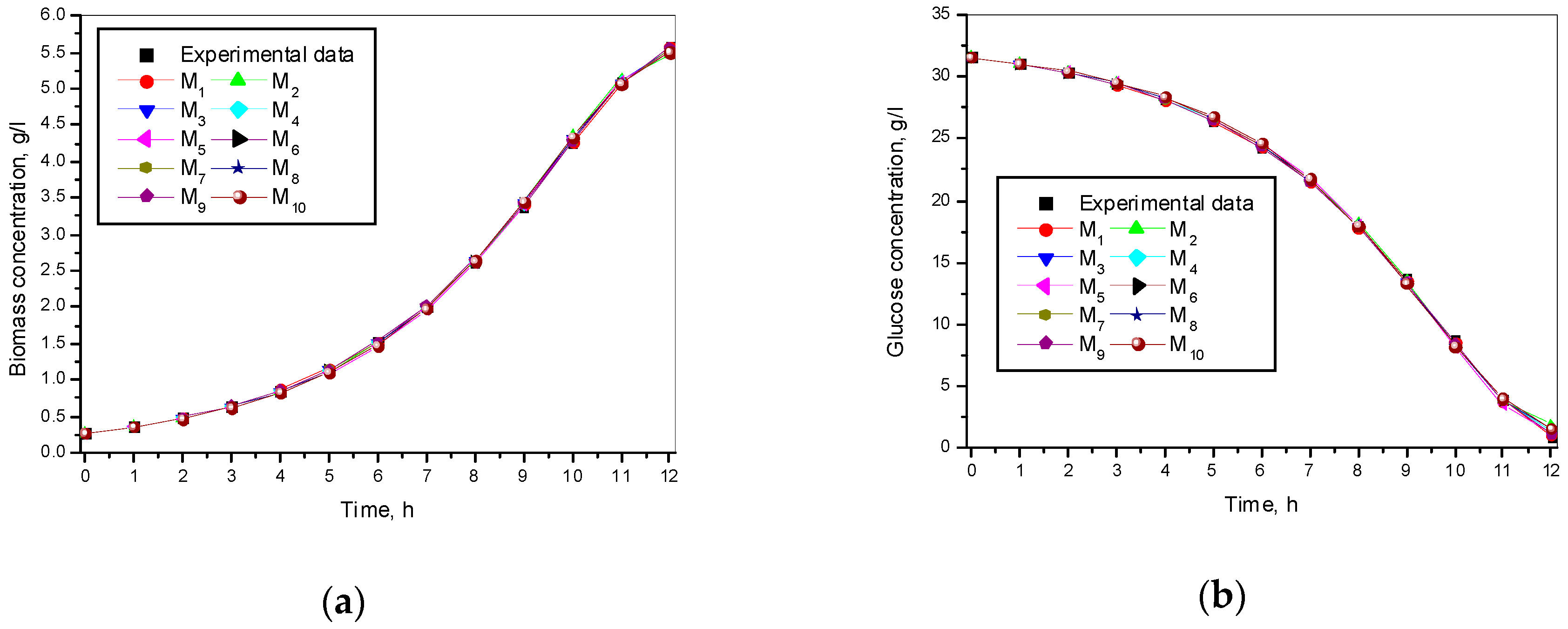
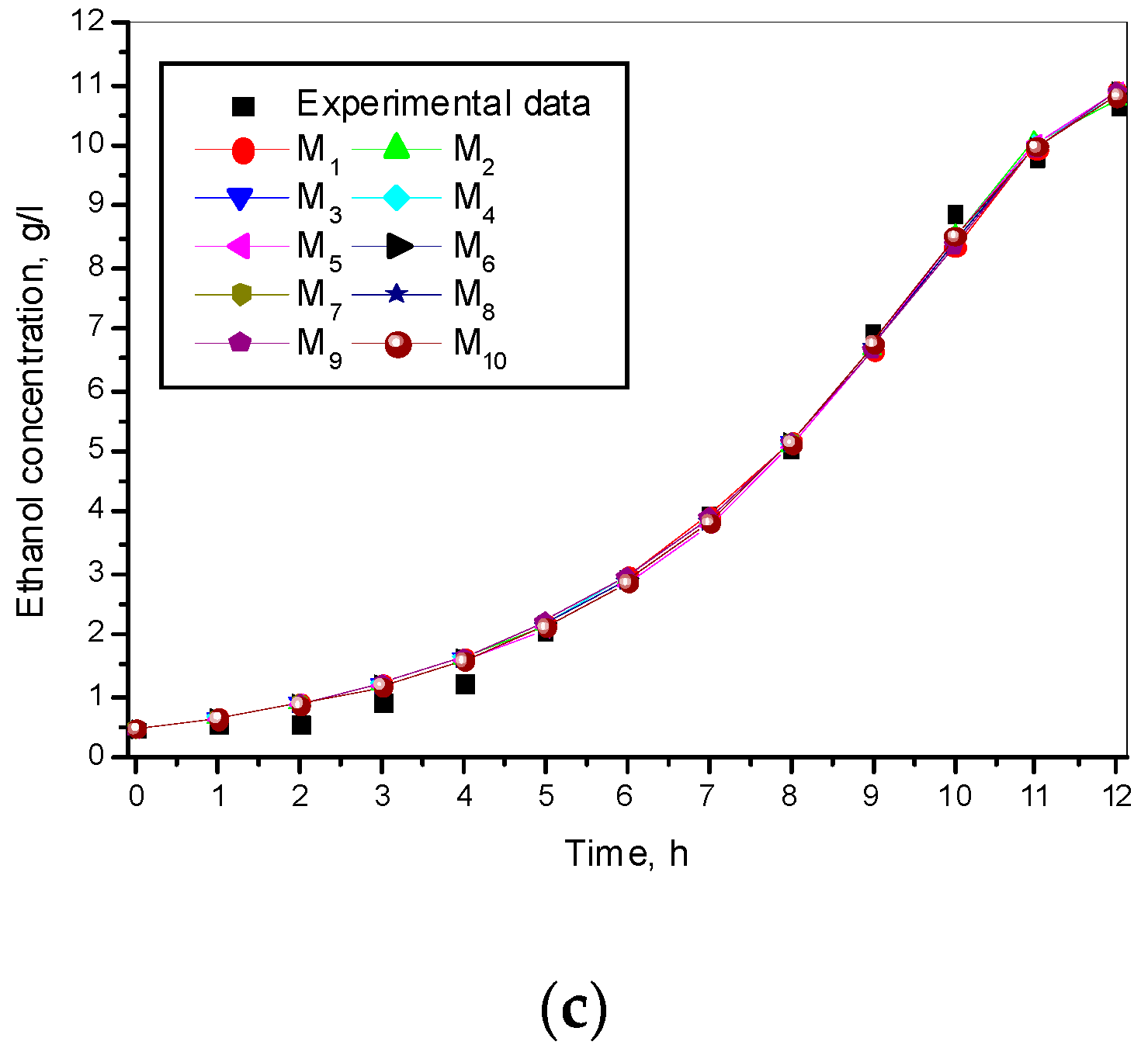
The experimental and simulated results of the model (1)–(3) and the ten models for a specific growth rate of
Saccharomyces cerevisiae are shown in
Figure 1.
Figure 1 shows different specific growth rate models and presents a very good match between experimental and simulated data for all the kinetic variables.
From the above (
Table 3 and
Figure 1), it follows that each model can be used to model a specific growth rate. By applying the PROMETHEE II method, we will select the most appropriate one.
3.2. Application of PROMETHEE II Method
3.2.1. Selection of the Weight
The criteria C1 are the most important. That is why we chose more weight for them (in %), or w1 ≅ 28%. The criteria of C2–C5 are important statistical variables. They show the statistic λ, and the relative error between experimental and simulated results. Their weight should therefore be higher than that of criteria C6–C11. For them, we chose six times the weight, or wj ≅ 14%, j = 2, …, 5.
From the results obtained, it could be seen that the criteria C6, C7, and C8 had approximately equal values and were very close to their minimum. The same applied for the criteria C9, C10, and C11. They were also close to their maximum. For all of them, we chose smaller weights, wj ≅ 3%, j = 6, ..., 11. The sum of all weights fulfilled the condition: Σwj ≅ 100%, j = 1,…,11.
3.2.2. Selection of the Preference Function
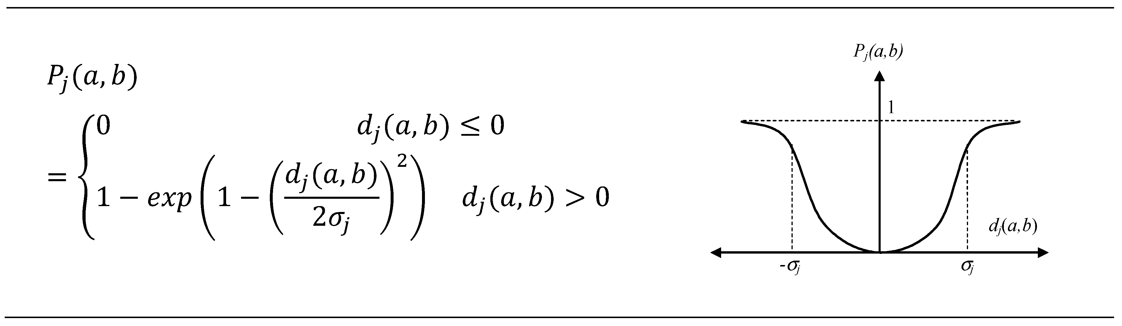
Choosing a preference function is a very important task. The criteria of
C1–
C5 are important statistical variables. As their value is close to zero, the best part of the results simulated by the models was selected for the experimental data. Very suitable for them was Type VI: Gaussian criterion (
Figure 2).
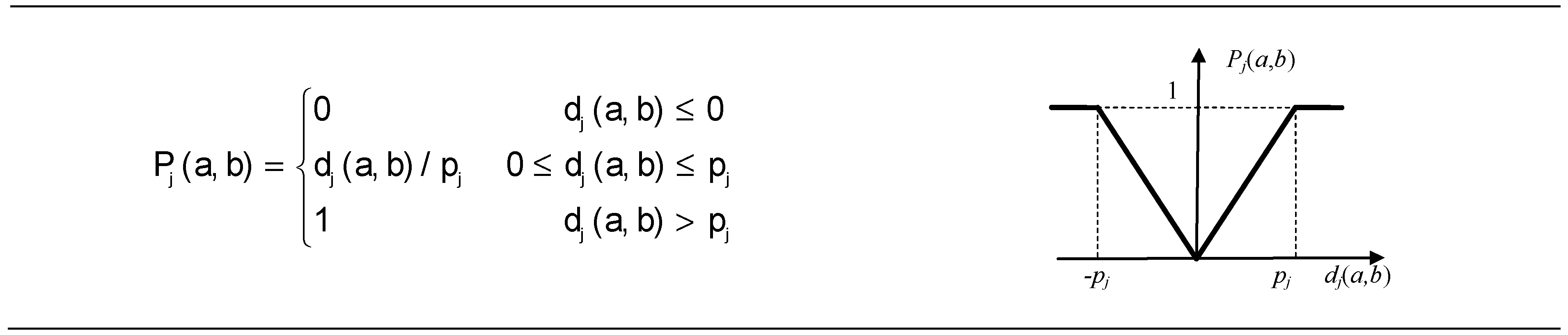
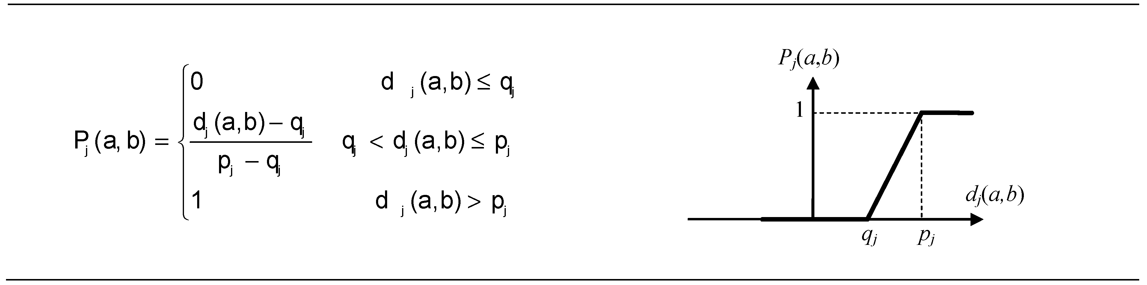
The
C6,
C7, and
C8 criteria were close to their minimum, and the preferred function of Type III: V-shape criterion was the most appropriate for them (
Figure 3).
The criteria
C9,
C10, and
C11 were close to their maximum. For them, the preferred function was Type V: V-shape with indifference criterion (
Figure 4).
3.2.3. The Software Packages
We used PROMETHEE Academic Edition software [
32] to solve the multi criteria decision-making problem.
Table 4 shows the preference function types and their parameters.
The results for different growth rate models when a PROMETHEE II method was applied are shown in
Table 5.
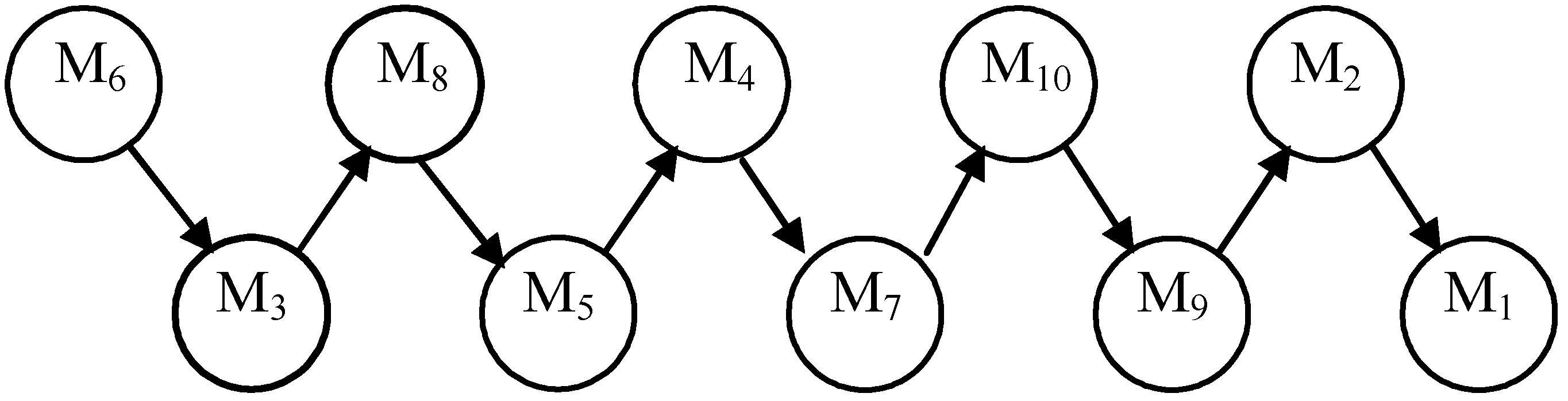
The total pre-order for the specific growth rate models is shown in
Figure 5.
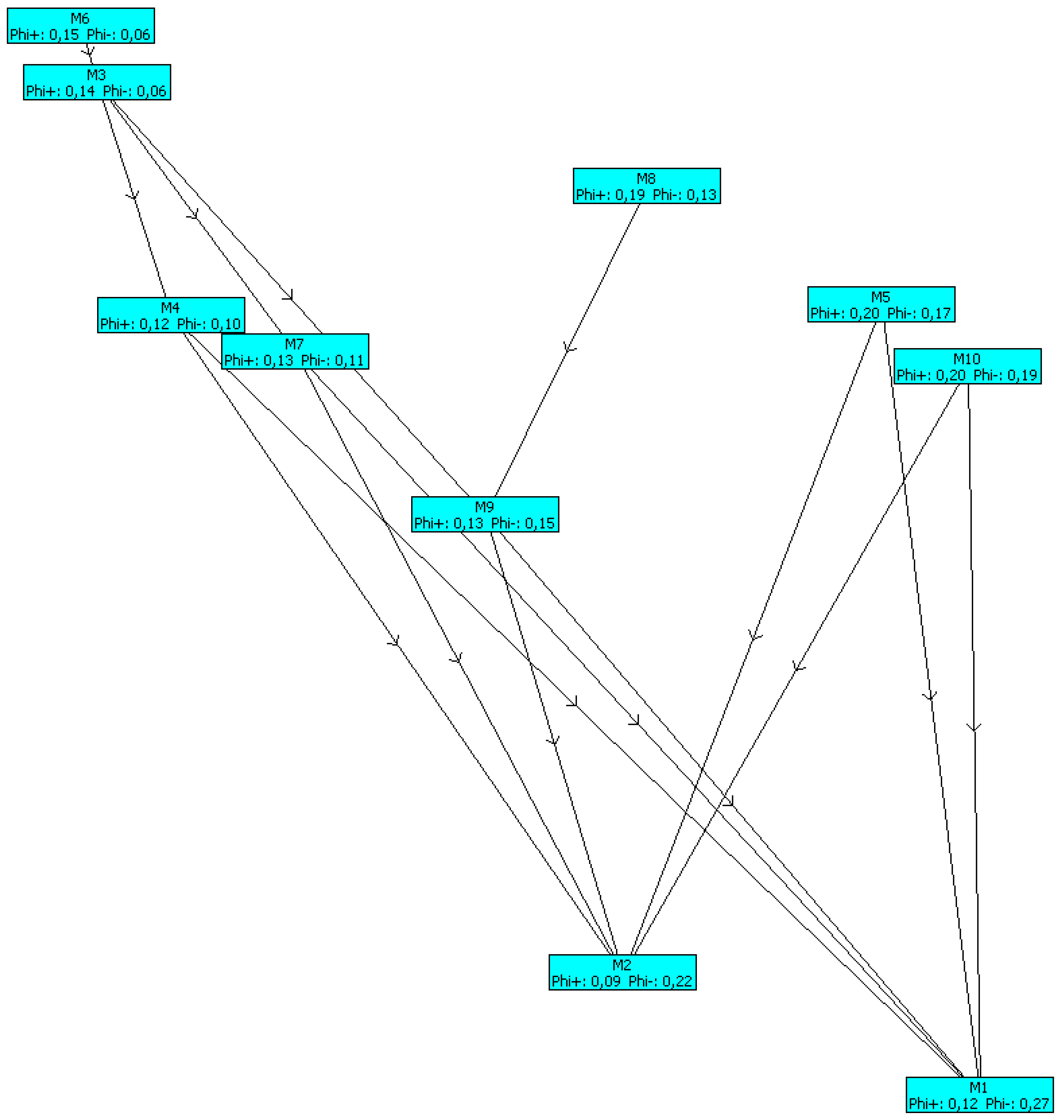
The results obtained (
Table 5,
Figure 5, and
Figure 6) showed that the Andrews model (M
6) was the highest ranked one. The mathematical model of the batch process of
Saccharomices cerevisiae with the Andrews model is shown below:
This model would be used to model the process. The parameters of models (10)–(12) were as follows: µm = 0.410 h−1; KS = 7.919, g/L; KSI = 249.365, g/L; YS/X = 0.173, g/g; YS/E = 0.507, g/g.
The PROMETHEE network is shown in
Figure 6.
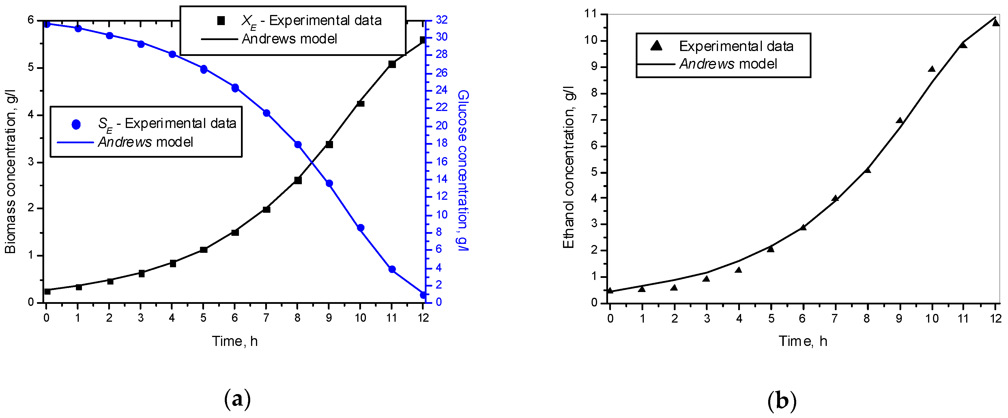
Figure 7 shows the experimental and simulated results achieved through (11)–(13) models, where
XE and
SE were the experimental data for biomass and glucose concentration.
The results presented in
Figure 7 show that the Andrews model described the experimental data very well. This is especially true for the simulation of the biomass and glucose concentration. In regard to ethanol, there were very few differences.
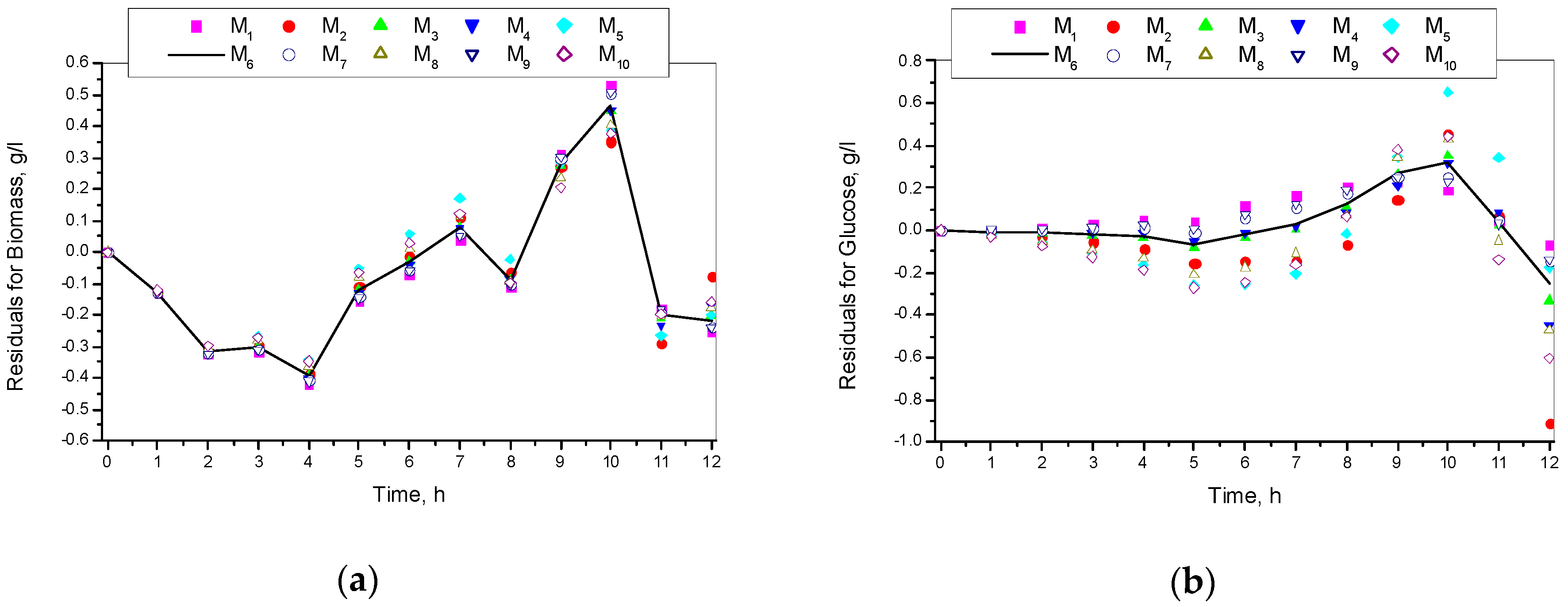
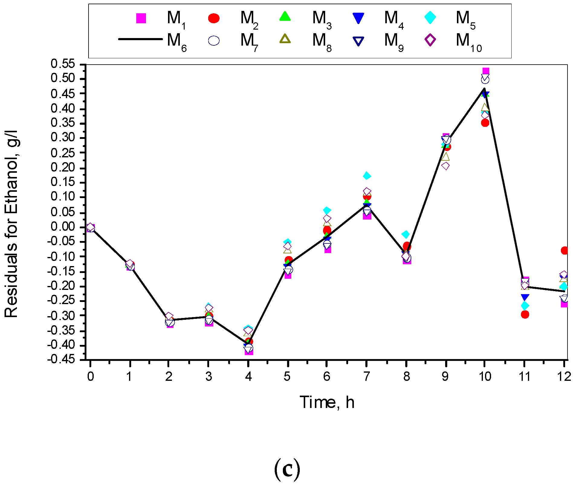
Figure 8 shows the residuals for all the ten specific growth rate models.
Figure 8 shows that residuals achieved through the Andrews model were medium in comparison to all other models. Therefore, it was a kind of compromise option to the rest and, last but not least, it had very good indicators.
4. Conclusions
The study presents different mathematical models of specific growth rate of a batch process of Saccharomyces cerevisiae yeast cultivation for ethanol production. Ten models were investigated for the specific growth rates: Monod, Mink, Tessier, Moser, Aiba, Andrews, Haldane, Luong, Edward, and Han-Levenspiel. The statistical results (the criteria of evaluation of the parameters in the models) and the statistical criteria (statistics λ, Fisher, and correlation coefficient) showed that all the investigated models were adequate.
Using the PROMETHEE II method showed that the most suitable model for specific growth rate dependent on glucose was the Andrews model, which would be used for modelling of the process.
The specification of the coefficients in this model will be done in another paper, where the identification will be done simultaneously for fed-batch cultivation. This model will then be used for modelling, optimization, and optimal control of batch and fed-batch processes for ethanol production, with the purpose of increasing the productivity of the ethanol.


