Article

Numerical Analysis of Multi-Particulate Flow Behaviour in CFB Riser Coupled with a Kinetic Theory

by
Fardausur Rahaman
1,
Abd Alhamid Rafea Sarhan
2,3,* and
Jamal Naser
2
1
SLR Consulting Australia Pty Ltd., Spring Hill, QLD 4000, Australia
2
Department of Mechanical and Product Design Engineering, Swinburne University of Technology, Hawthorn, VIC 3122, Australia
3
Department of Biomedical Engineering, University of Melbourne, Melbourne, VIC 3010, Australia
*
Author to whom correspondence should be addressed.
Fluids 2023, 8(9), 257; https://doi.org/10.3390/fluids8090257
Submission received: 26 July 2023 / Revised: 30 August 2023 / Accepted: 4 September 2023 / Published: 21 September 2023
(This article belongs to the Special Issue CFD-DEM Modelling of Multiphase Flow)

Abstract

:
In this work, a three-dimensional CFD model for the gas–solid flow of two different particle sizes in a CFB riser coupled with a kinetic theory (KT) has been developed. The properties of the solid phases are calculated using the proposed multi-particle kinetic theory. The CFD model is implemented in the commercial CFD software CFX4.4. In the current model, one gas phase and two solid phases are used. However, the model is generalised for one carrier phase and N number of solid phases to enable a realistic particle size distribution in the system. The momentum, volume fraction and granular temperature equations are solved for each individual solid phase and implemented into the CFD model through user-defined functions (UDFs). The k-ε turbulence model is used in simulating the circulating fluidised bed model. For verification, simulation results obtained with the new KT model were compared with experimental data, and then the model was used for further analysis. It was found that the proposed multi-particle model can be used to calculate the properties of gas–solid systems with particles of different sizes and/or densities, removing the assumptions of previous models that required all the particles to be of an equal mass, size and density.

1. Introduction

Gas-fluidised bed reactors are frequently used in many important industrial processes, especially in the oil industry [1,2,3], mineral processing [4,5] and electric power generation industries [6] due to their excellent heat and mass transfer characteristics, on the one hand, and solid mobility, on the other hand. Despite its widespread application, the hydrodynamics of gas-fluidised beds, unfortunately, remains poorly understood. This lack of understanding poses a significant obstacle to the up-scale of industrially important reactors [7,8,9]. Computational Fluid Dynamics (CFD) is a powerful tool for gaining a theoretical understanding of the complex multiphase flow and transfer processes in reactors [10,11,12]. However, CFD has not matured enough to predict the flow behaviour of a gas–solid flow system containing solids of different sizes and densities.
Much progress has been made in recent years towards developing computer codes for describing the hydrodynamics of gas-fluidised beds. Most of the developed models are based on a two-phase description, one gas and one solid phase and all the particles are assumed to have one diameter, density and a coefficient of restitution [13,14,15,16]. However, in real particle systems, particles of different sizes and densities exist; furthermore, the operation of many industrial processes is strongly dependent on having different particle sizes in the reactors. For such systems, a multi-particle approach is required for modelling and describing this class of gas–solid flow systems. There are some studies available in the literature [17,18,19,20] where different sizes and densities of particles were considered as different phases. However, due to the limitations of their models [3], none of them can be used to predict the behaviour of a multi-particle system. For example, Bell (2000) and Manger (1996) [17,18] extended the kinetic theory to binary mixtures of solids with unequal granular temperatures for the phases. In these models, fixed viscosities were used for each solid phase, and an interphase momentum transfer term was derived to account for the momentum transfer between solid phases due to collisions. However, arbitrary constants were used in determining the number of collisions. As the number of collisions can be obtained from kinetic theory, the kinetic theory approach would appear to be superior [21,22].
As highlighted earlier, many existing models have been tailored for single-particle flow scenarios [23,24,25,26,27,28,29]. Consequently, the capacity to forecast the intricate flow dynamics of particles of varying sizes within a gas–solid flow framework remains a notable deficiency, leading to considerable inaccuracies in the advancement and upscaling of gas–solid flow systems such as fluidised beds. In light of this, the principal objective of this study is to pioneer a multi-particle Computational Fluid Dynamics (CFD) model designed for a Circulating Fluidised Bed (CFB) while scrutinising the intricate flow behaviours of diverse-sized particles. In order to address this gap, the current work leverages the kinetic theory of the model introduced by [
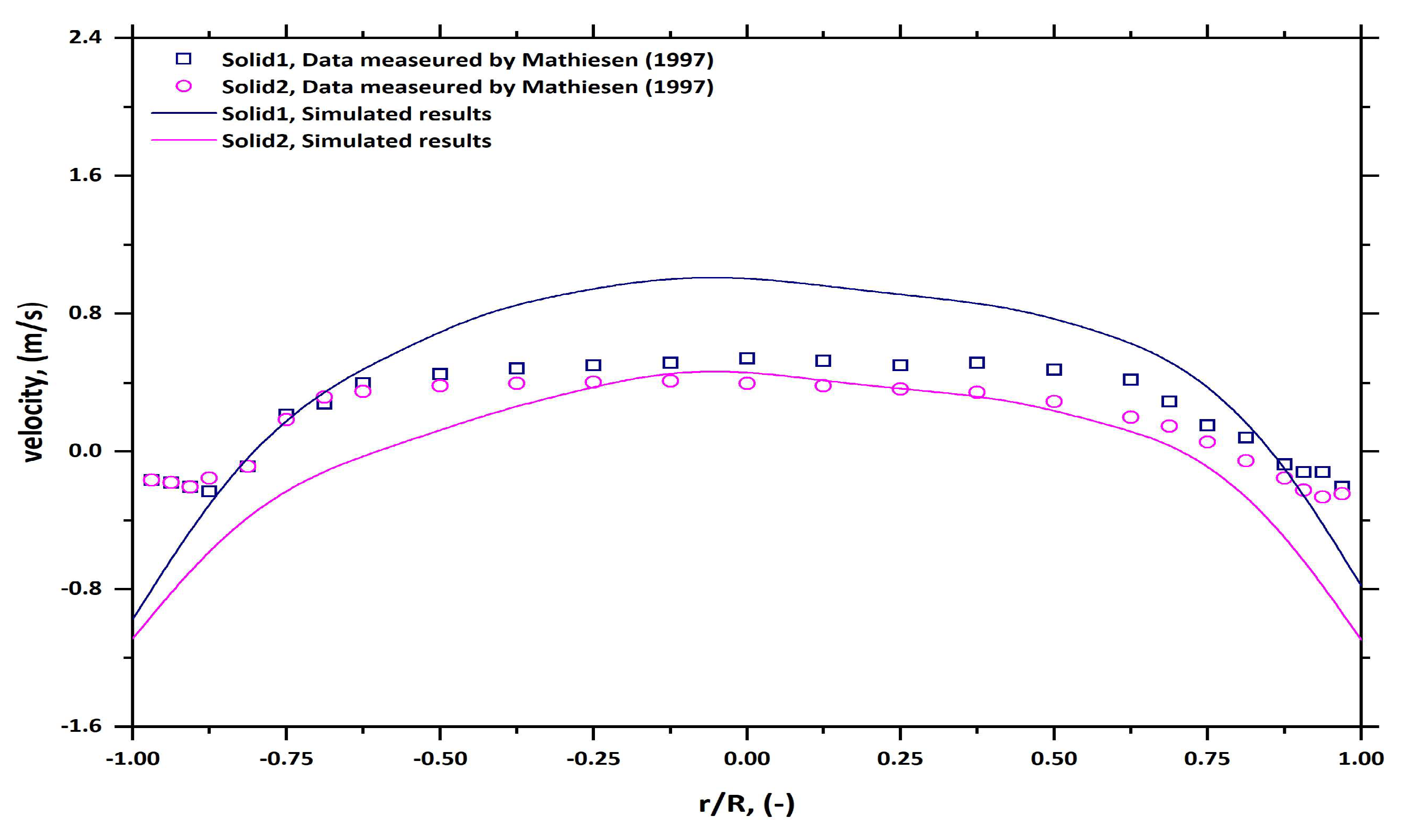
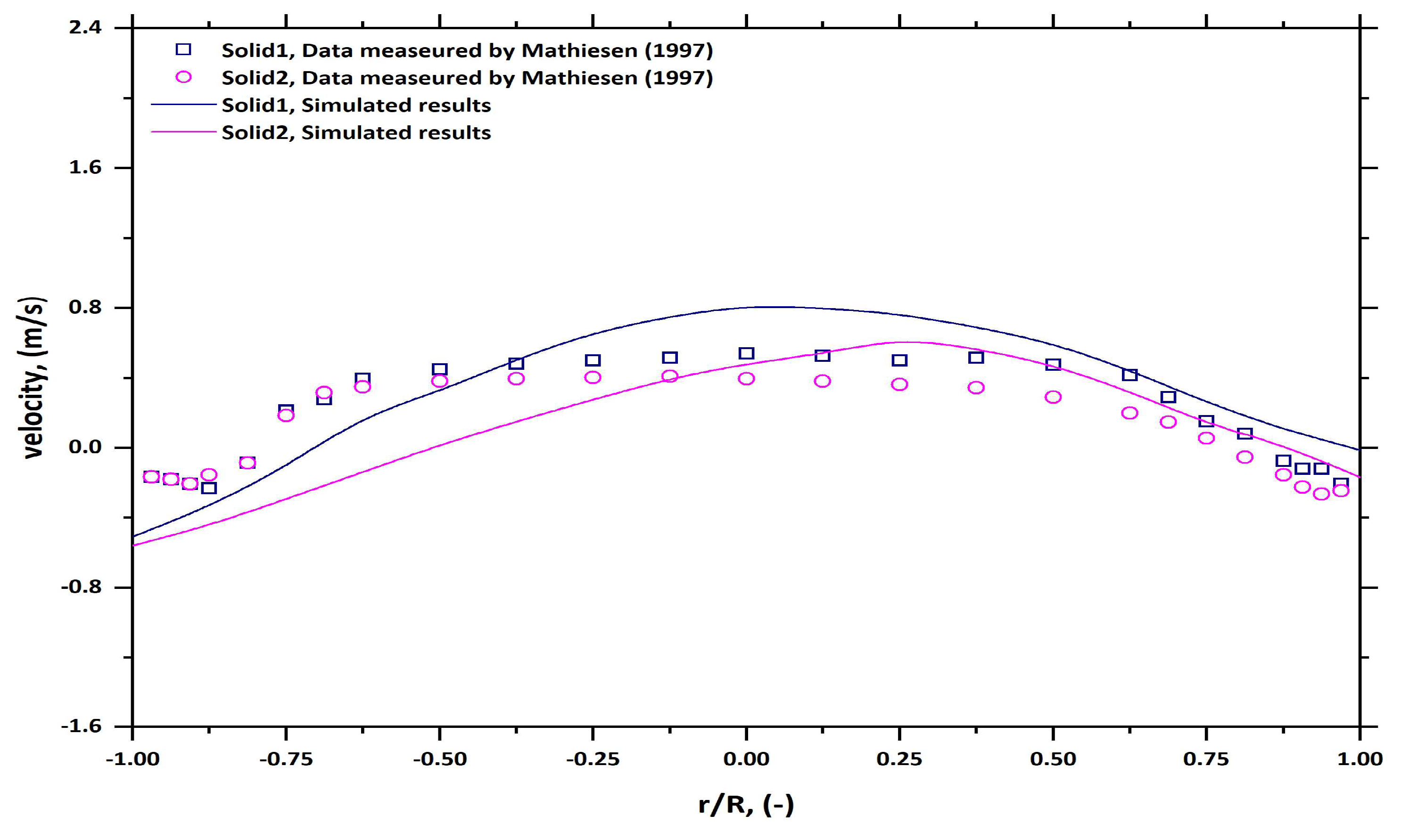
3] to simulate the behavior of a CFB riser. This kinetic theory model exhibits its versatility in accommodating multi-particle systems, where variations in particle mass, diameter, restitution coefficient, density and granular temperature are considered. Notably, the model takes into account the heterogeneity of particles and encompasses diverse flow characteristics within solid phases, including solid viscosity, solid pressure, collisional heat flux and bulk viscosity, stemming from intricate particle–particle interactions. For this investigation, the chosen CFB configuration aligns with a previous study conducted by Mathiesen in 1997 [30], thereby establishing a solid foundation for the ensuing analysis.
As previously mentioned, most of the developed models are applicable to a single particle flow system [23,24,25,26,27,28,29]. Thus, the ability to predict the flow behaviour of different-sized particles in a gas–solid flow system is still lacking, which causes significant errors in the development and scale-up of gas–solid flow systems such as fluidised beds. Therefore, the main objective of the present study is to develop a multi-particle CFD model for a Circulating Fluidised Bed (CFB) and analyse the flow behaviour of different-sized particles. The kinetic theory model developed by [3] is used in the present work to simulate the CFB riser. This model is applicable to multi-particle systems, where the mass, diameter, restitution coefficient, density and granular temperature of the particles may be unequal. Different flow properties for solid phases (such as solid viscosity, solid pressure, collisional heat flux and bulk viscosity) resulting from particle–particle interactions are obtained from the multi-particle kinetic theory. The CFB that has been selected for investigation was previously tested by Mathiesen (1997) [30].

2. Mathematical Model

Detailed development of the multi-particle kinetic theory, along with mathematical comparison with other available theories in the literature, has been presented in our previous publication [3,21,31]. This theory has been implemented in the commercial CFD software CFX and used to simulate the riser section of a circulating fluidised bed having particles of different sizes. Two different particle species have been considered. Particles of each species are considered smooth, elastic and homogeneous spheres. Different flow properties for solid phases (such as solid viscosity, solid pressure, collisional heat flux and bulk viscosity) resulting from particle–particle interactions are obtained from the multi-particle kinetic theory. Interphase transfer terms (momentum transfer, fluctuating energy transfer) between the solid phases are also added to the code through the user subroutine. In the present model, we employed the standard k-epsilon turbulence model to simulate the experimental results. The choice of this turbulence model was motivated by its widespread use and applicability to a wide range of engineering scenarios. The k-ε model is well-suited for capturing turbulence characteristics and flow phenomena in various configurations, making it a suitable candidate for our investigation. A comparison of predicted results with experimental results validates the model [32]. The CFB that has been selected for investigation was previously tested by [30]. Details of the governing equations used in the simulations and the model formulation are summarised in Table 1 [3]:
Reynolds-Averaged Navier-Stokes equations (RANS) were used in the study (please refer to Table 5). RANS equations are only mentioned in Table 5 and not elaborately presented here in this paper, as the use of RANS Equations is standard practice in CFD. The standard k-ε model was used in this study (Table 5). In the Standard k-ε model, the eddy viscosity is computed from turbulent kinetic energy and turbulent dissipation. This eddy viscosity is used in RANS Equations. The electrostatic forces between the particles were ignored in the present study.
In the present model, the transport equations were discretised using the finite volume method (FVM). To discretise the convective term, we employ a second-order upwind scheme. This scheme is known for its ability to capture the directionality of flow and minimise numerical diffusion, especially in cases of high gradients. The diffusive term was discretised using a central differencing scheme, which provides second-order accuracy. This scheme is suitable for capturing diffusion effects accurately and maintaining stability. The source term was treated implicitly to ensure stability and accurate representation of the physics. We use the SIMPLE (Semi-Implicit Method for Pressure-Linked Equations) algorithm to handle the pressure-velocity coupling and ensure the pressure-velocity decoupling is carried out efficiently.

3. The CFB System

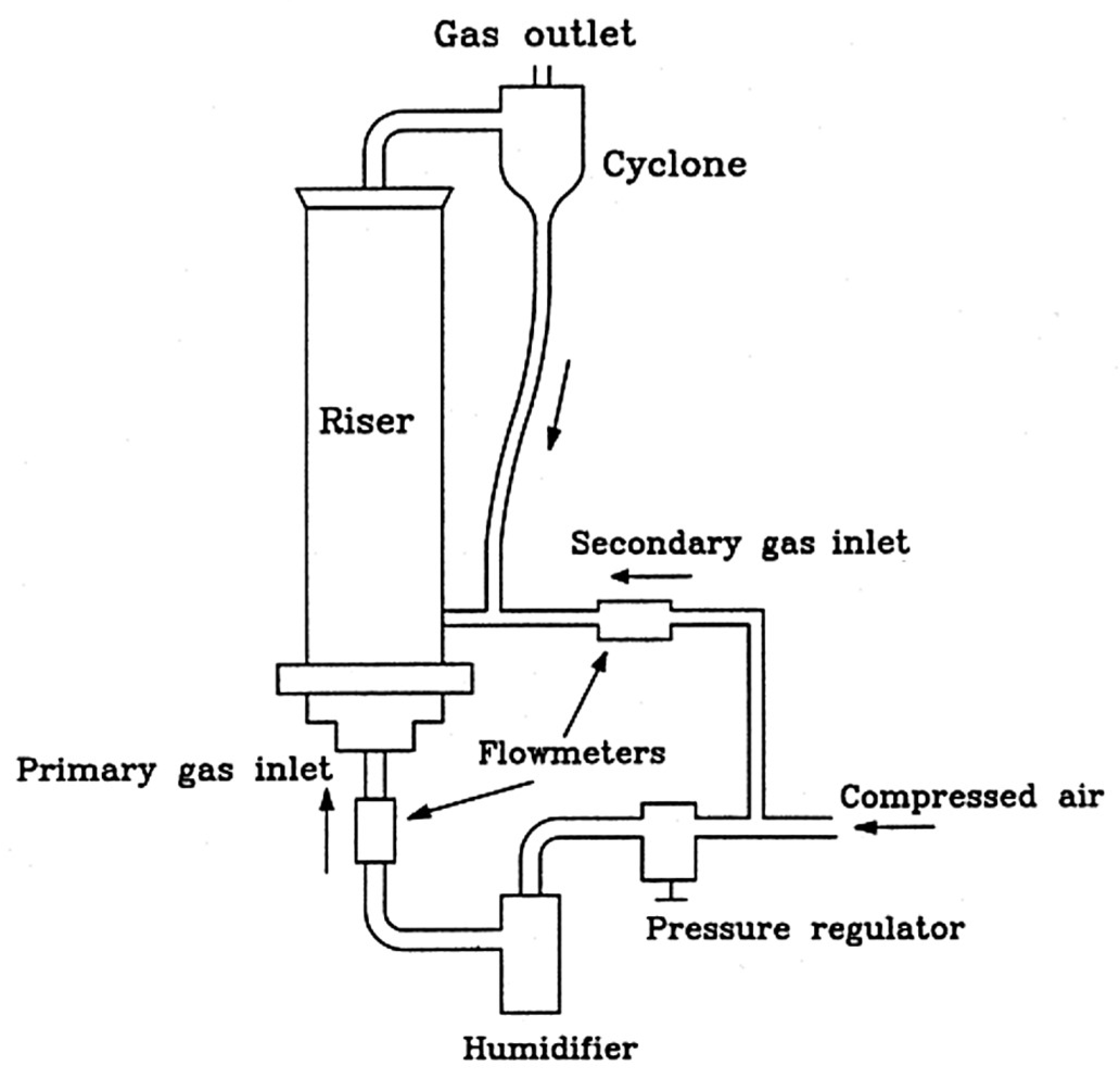
The CFB system experimentally investigated at Telemark Institute of Technology is shown in Figure 1. The riser was cylindrical in shape with an internal diameter of 0.032 m and a height of 1.0 m. The primary gas inlet was located at the bottom of the riser. In order to provide a uniform gas velocity at the inlet, an air distributor was installed. The distributor was a Duran filter plate with a thickness and porosity of 0.004 m and 0.36, respectively. At the top of the riser, the suspended particles enter a glass cyclone where the solids are separated from the gas and recycled via a return loop. Supply of secondary air positioned at 0.05 m above the air distributor feeds the solids back to the riser. Figure 1 shows a schematic sketch of the circulating fluidised bed system used in the experiment.
Two distinct particle groups were sieved out from a Gaussian particle size distribution with a Sauter mean diameter of 157 μm. The diameters of the sieved particles are between 100 and 130 μm and between 175 and 205 μm for the smallest and largest particles, respectively. The mean particle diameters of the two groups were approximately 120 and 185 μm. The two distinct groups were mixed together, and the initial volume concentration of each group was identical. The particle density was 2400 kg/m3. The initial bed height was 0.04 m. Thus, the overall volume concentration of solids in the riser is 2.5%. The flow parameters used in this work have been shown in Table 2.

4. Grid and Physical Domain

Only the riser part of the circulating fluidised bed shown in Figure 1 has been modelled. In order to avoid convergence difficulties, the calculation domain is divided into five blocks. The grid characteristics and the grid information are listed in Table 3 and Table 4.
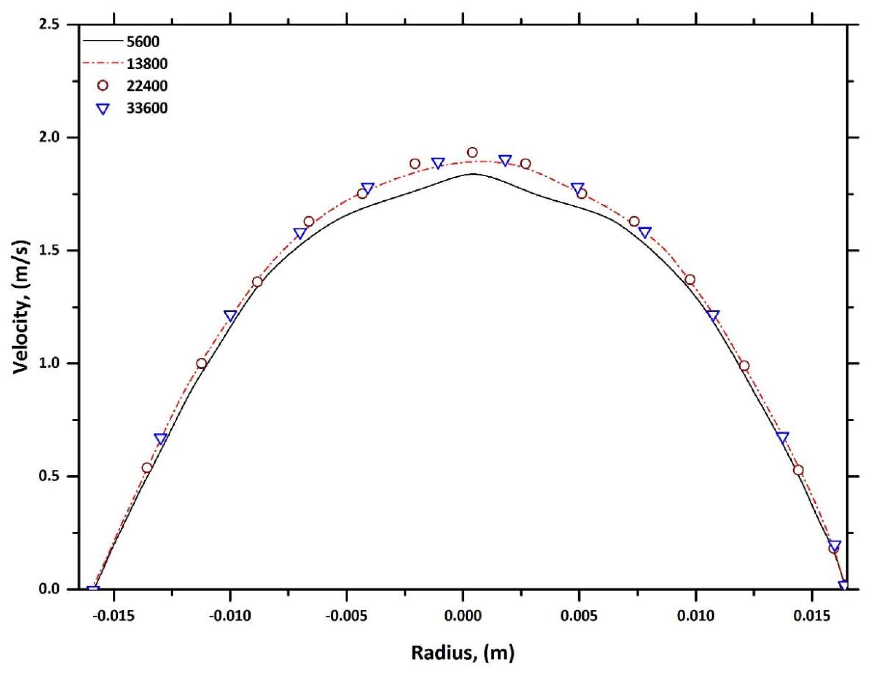
The grid independence test was performed for this study through the simulation of gas flow in the riser. Starting with a lower number of cells of 5600 in the riser, the number of cells in the riser was extended up to 33,600 in four steps. The calculated results for each step have been shown in Figure 3. It has been observed from Figure 3 that with the increase in cell number beyond 22,400, the velocity is independent of the number of cells. Therefore, for this study of the riser flow CFB, 22,400 cells have been used for further simulations. In this test, mass source residual (error in continuity) is used to control the convergence of the solution, and the tolerance limit was set to 10−6. In this simulation, the equation for continuity, momentum and transport equation for k and ε were solved for turbulence parameters.

5. Boundary and Initial Conditions

In this work, a wall boundary, inlet and outlet boundaries are used. The inlet boundaries are given by a specific inflow velocity and volume fraction. The inlet velocity and volume fraction used in this simulation are given in Table 2. At the outlet, a pressure boundary condition with atmospheric pressure has been used. This essentially applies constant gradient conditions to the flow variables. Solids are also permitted to leave through the boundary. Buoyant flow has been enabled with gravity of 9.81 m/s2.
For a gas, the no-slip wall condition is well accepted and used. However, for walls that are both non-slip [17,33] and free-slip [34], solid velocity conditions have been used by different researchers. In general, it is not permissible to set the particle velocity equal to zero at a solid wall. Exceptions occur when the wall is sufficiently rough, minimising particle slip and when the bounding wall is sufficiently soft, creating highly inelastic particle–wall collisions. Tsuo and Gidaspow [35] used a partial-slip boundary condition, which is between the two mentioned conditions. Insufficient numerical and experimental work has been undertaken to show any boundary condition as being superior with all capable of predicting clusters. In non-slip boundary conditions near the wall, some fluid (for example, a layer of fluid molecule/molecules) is assumed to attach to the solid wall, whereas in no slip boundary condition, fluid does not attach to the solid wall. Slip boundary conditions are used to model the behaviour of particles near solid surfaces, where the particles experience a slip velocity relative to the fluid due to a lack of adhesion. The choice of slip condition can indeed influence the results of simulations, and using different slip models, such as partial slip conditions or incorporating slip lengths, could provide valuable insights into the role of slip in the observed deviations. In our study, we chose a slip boundary condition based on the available literature and its relevance to the specific system we were simulating.
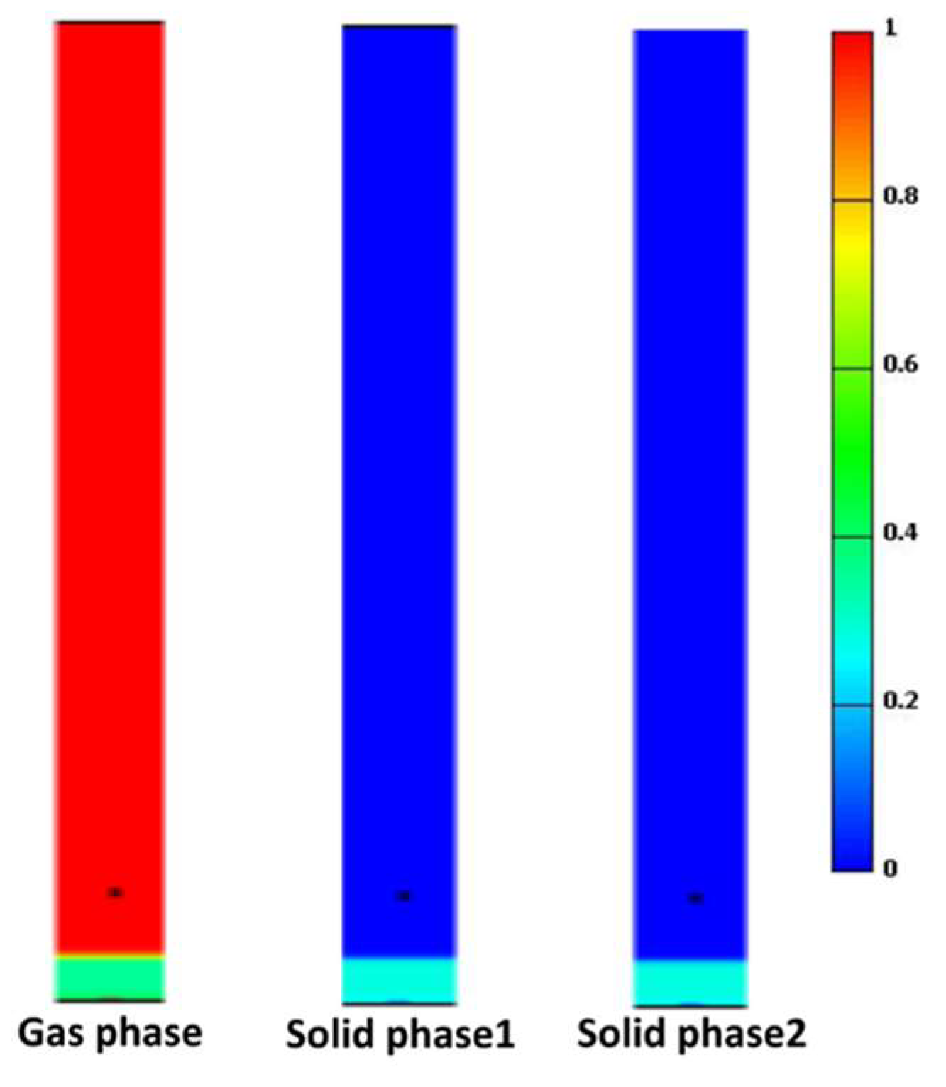
In this work, the riser is initially filled with a 0.04 m high bed where the total volume fraction of solids is approximately 0.63. The initial volume fractions for each individual phase have been show in Figure 2. The two solid phases are perfectly mixed in the bed and are assumed to have an identical initial volume fraction. In order to avoid convergence difficulties, the initial volume fraction of the solids above the bed in the computational domain is set to 1.0 × 10⁻¹⁰, and to ensure a small initial viscosity, the granular temperature has been set to 1.0 × 10⁻¹⁰ in this work.
The proposed multi-particle kinetic theory of [3,21,31] was implemented in the commercial CFD code CFX through user subroutines. A time step of 0.001 s is used for the calculations. The under-relaxation factor used for the velocities and volume fraction was 0.3, and for the granular temperature, it was 0.2. Typically, 32.5 h of computational time is required on an Intel Pentium 4 (Xeon) 2.0 GHz computer to simulate one second of real-time. A summary of the model formulation used in the present work is introduced in Table 5.

6. Results and Discussion

6.1. Solid Velocity Profile

Figure 4 shows the instantaneous velocity vectors at 21.0 s for the gas and the solid phases. The solid phase with smaller diameter (120 μm) particles is classified as Solid1, and the solid phase with a larger diameter (185 μm) has been classified as Solid2. A subsection of the physical domain has been enlarged in order to illustrate the flow pattern. A close-up view of the velocity vectors for gas, Solid1 and Solid2, are shown in Figure 3, respectively.
In studying Figure 4, it has been observed that the flow pattern for both solid phases is a core–annulus type of flow. A similar trend was found by [24,35,37]. Near the centre of the riser, there is an upward, rapidly moving core surrounded by a downward, relatively slower-moving annulus near the wall. The flow was started with a packed bed of solids at the bottom of the riser. Initially, the solids and the gas moved uniformly in a plug flow mode. Skin friction for air at the wall modified the flow by reducing the velocity in the near-wall region. The imposed velocity gradient caused by the wall pushed the particles towards the wall in the radial direction. This caused cluster formation, and particles started accumulating in the form of clusters in the near wall region. The cluster behaves as a hydrodynamic unit or as a particle of large effective diameter. Hence, the gravitational force acting on the cluster becomes higher compared to the drag force, and particles start to move downwards. Figure 4 shows these negative velocities of the clusters. Thus, an annular region formed near the wall. In order to conserve the inlet constant mass flow, the upward velocities for both the gas and the solid phases in the core region had to increase in order to compensate for the additional area occupied by the downward-flowing annular region. Eventually, the upward and downward flow reaches a quasi-equilibrium state.
From Figure 4, it can be observed that the velocity on the right side of the core is higher as compared to the velocity on the left side of the core for both gas and solid velocities. As Figure 4 illustrates, with the instantaneous velocities, some local variations are expected due to the influence of transient void distribution in the riser. However, when the mean velocities for the gas as well as the solids were plotted, the ideal core–annular flow can be observed, as shown in Figure 4. This core annular flow pattern shows that all three phases are moving upward through the central region. However, the velocity of the gas is higher than that of the solid phases. It should also be noted that the Solid1 particles move faster than the Solid2 particles. Figure 5 also clearly shows that particles are falling down under gravity along the wall, whilst in the centre of the riser, a core of upward-moving gas and diluted solids has been formed. Particles with a smaller diameter (Solid1) travel at higher velocities when compared to the particles with a larger diameter (Solid2) in both core and annular regions. This is due to the smaller gas–particle drag force required to accelerate the particles of smaller diameter. A similar trend was found in Mathiesen and Solberg‘s [20] experimental data under identical conditions. It has been observed from Figure 6 that with the increase in height, the width of the core region increases, which is consistent with observations of [38].
Figure 6 and Figure 7 show the transient velocity variation in the solids with time at different heights, low x, centre and high x of the riser. Results presented in these figures show a similar behaviour near both walls with substantial fluctuations present in both solid phases. The Solid1 velocity predicted near the riser walls (low and high x) oscillates between an upward velocity of 0.3 m/s and a downward velocity of 0.6 m/s. However, in the centre, the solid velocity oscillation is higher compared to the oscillations near the wall. Near the centre, the Solid1 particle velocity fluctuates between 0 m/s and 3 m/s in an upward direction. The Solid2 velocity predicted near the riser walls (low and high x) oscillates between an upward velocity of 0.1 m/s and a downward velocity of 0.7 m/s. Near the centre, the Solid2 particle velocity fluctuates between 0 m/s and 2.5 m/s. Significant oscillations of the velocities with time were observed in Figure 6 and Figure 7. As Figure 6 and Figure 7 illustrate for the instantaneous velocities, some local variations are expected due to the transient nature of the system, resulting in velocity fluctuations. Similar trends were found in single-phase fluidised bed models by [16,33]. For multi-particle flow, measurements of the velocity variation with time along the wall region are not available in the literature, making validation of these predictions of wall velocity difficult. Figure 6 and Figure 7 confirm a stochastic flow behaviour in the riser. The particle’s velocity is almost always negative, close to the wall. In the central part of the riser, the oscillating velocity includes negative and positive values, but a much higher fraction of the particles is flowing upward than downward.

6.2. Validation of the Numerical Results

Figure 8 shows the measured and computed particle velocity profiles for both solids (Solid1 and Solid2). The particle velocity profiles are obtained with a superficial gas velocity of 1.0 m/s and are at a height of 0.4 m above the gas inlet. As discussed earlier (Section 6.1), core–annulus flow is predicted in the riser. The behaviour is clearly observed in the simulation as well as the experimental work of [20,30]. The measured velocity profiles show a relative velocity between the two solid phases in the core region. In the wall region, no significant relative velocity was observed on the left side of the experimental velocity profile, and significant relative velocity was observed on the right side of the experimental velocity profile. However, the computed results indicate a significant relative velocity between the solids in the core region as well as in the wall region. The relative velocity is expected in the core region as well as in the wall region. The relative velocities are caused by different values of gas–particle drag for the different-sized particles. The particle–particle drag, which is a function of the particle–particle collisions, will also play a major role in determining the magnitude of the relative velocity.
Though the proposed model correctly predicted the velocity trend in the core region, it can be observed that it has over-predicted the downward velocities of the solids in the near-wall region. This over-prediction of the downflow velocities may be due to the fact that electrostatic forces were present in the experiments and were not incorporated into the model. As mentioned earlier, Miller and Gidaspow [38] reported the presence of much static electricity in the CFB system. Their observation shows that the particles were attracted and almost glued to the wall were observed. Another cause may be in the selection of wall boundary conditions. In this work, the free slip boundary condition was used for the solid phases. The use of partial slip boundary conditions might provide a better prediction in the wall region. In the core region, this model correctly captures the trend of the velocity. The magnitudes of the velocities are in reasonably good agreement with the experimental results. It has been observed that the model over-predicts the velocity of Solid1. However, the predicted velocity of Solid2 is in good agreement with the experimental results. This may be attributed to the gas–particle drag model used in this study.
The results of Mathiesen [30] for particles of different sizes are reproduced in Figure 9. A comparison of Figure 8 and Figure 9 shows that the proposed model can capture the trend of the velocities more preciously than Mathiesen’s model in the core region. However, in the annular region, the Mathiesen [30] model provides a better prediction compared to the proposed model. This is due to the wall boundary condition used in the model, as discussed in Table 5. In this model, a slip boundary condition was used. However, in Mathiesen’s model, a no-slip boundary condition was used. The use of partial slip boundary conditions might provide a better prediction in the annular region. It has been observed from Figure 8 and Figure 9 that both models predict higher relative velocities between the solids compared to the experimental prediction. The reason behind this might be the gas–particle drag model, as mentioned earlier in this section. Another reason may be the uncertainty of the mean diameter of the particle size distribution reported by Mathiesen [30]. A small error in the mean diameter may give rise to a significant rise in the drag terms, causing the over-prediction of the velocities. Since no other experimental data for a gas–solid flow system with different-sized particles are available in the literature, a more detailed validation of the proposed kinetic model is not possible at this stage. Though some variations in the magnitude of the solid velocities are observed compared to the experimental results, the proposed model predicted the trend of the velocity profile more accurately than the earlier models. To obtain better validation of the model requires better quality experimental data for a system with two single particle sizes and greater details of solid volume fraction, pressure drops and gas velocity.

6.3. Volume Fraction Profile

Figure 10 shows the computed radial time-averaged volume fraction profiles of solids at different riser heights. Time-averaging was performed over the last two seconds of the 21 s of the real-time simulation. This was selected in order to isolate a period of relative stability and relevance to the observed system’s behaviour. This approach enhances the accuracy of the comparison with experimental data and provides a clearer understanding of how well the model aligns with real-world dynamics. At all locations, the solid volume fraction distribution shows the expected trend, a dilute region in the core and denser flow near the wall. As expected, the solid concentration is highest near the base of the riser at 0.05 m and decreases with the increase in height. Since no experimental data for volume fraction are available, no comparison with the experimental results can be shown. The simulated volume fraction profile shows the trend of core–annular flow. Similar trends were observed in other numerical and experimental model results [33,38] for mono-particle flow in a CFB riser. At 0.05 m height, the solid volume fraction at the right riser wall is predicted to be higher than that at the left riser wall. The reason for this occurrence has been explained later on in this section.
Figure 11 and Figure 12 show the computed volume fraction distribution at different time intervals between 20 and 21 s for Solid1 and Solid2. In Figure 11, a cluster and gas void formation can be observed at different time intervals for Solid1. At 20.1 s, the formation of the gas void is observed near the bottom of the riser. With the increase in time, the formatted void expands up the riser, with the gas gradually tunnelling through the solids. This gas–solid interaction causes the solid material to separate towards the walls, resulting in a lower concentration of solids close to the centre of the riser and an increase in solid concentrations towards the walls. In the region close to the wall, cluster formation can be observed, and the solid particles move downward under gravitational force. Hence, a circulation of solids can be observed in the riser with a strong upward flow of the solid at the centre, gradual migration of solids towards the wall and a downward flow of solids in the near wall region. Figure 12 illustrates the Solid2 volume fraction in the lower section of the riser. It can be observed from Figure 12 that most of the solids remain at the bottom of the riser in the form of a turbulent bed, indicating particle separation.
The mention of particles being recirculated downwards in the lower half of the riser indicates that there’s a tendency for particles to move downwards instead of uniformly rising. This phenomenon can be attributed to the complex interplay of various hydrodynamic forces and particle interactions in the riser. The interaction between these forces and the particles themselves contributes to the observed behaviour. For instance, particles might collide and clump together due to these forces, causing them to become denser and heavier. As a result, these denser clusters tend to settle in the lower portion of the riser, counteracting the upward flow. This interplay of forces and particle behaviours leads to a non-uniform distribution of particles, ultimately causing the widening of the core region with an increase in height. Understanding this intricate relationship between hydrodynamics and particle interactions is crucial to comprehending the complex behaviours observed in the system.
Figure 13 and Figure 14 show the transient fluctuation in the solid’s volume fraction at different heights and at the riser centre line, low x and high x. It has been observed from the figures that with the increase in height, the solid volume fraction fluctuation decreases, which is expected as solid velocity reduces with the increase in height. By studying Figure 13, it can be observed that at 0.2 m height, near the centre of the riser, the Solid1 concentration fluctuates more compared to that at 0.4 m and 0.6 m height. In near-wall regions (low and high x), the solids fall down under gravity and return to the bottom of the riser. At the bottom, the returned solids move upward with incoming gas in the form of clusters. With height, the solid materials separate towards the wall as the gas gradually tunnelling through the solids. Therefore, in the lower section of the riser, 0.2 m, more cluster formation can be observed and hence, higher fluctuations in the solid volume fraction are expected when compared to that in the upper section of the riser. Figure 14 illustrates the Solid2 volume fraction in near-wall regions (low and high x) as well as close to the centre region. In Figure 14, a similar trend to that of the Solid1 volume fraction (Figure 14) can be observed for the Solid2 volume fraction. However, the Solid2 volume fraction at the upper portion of the riser is very low due to the greater particle diameter and, thus, has a higher terminal velocity.

6.4. Granular Temperature Profile

Figure 15 shows the time-averaged granular temperature distribution for both solid phases at different heights. It can be observed from Figure 15 that the granular temperature for lighter particles (Solid1) is reasonably uniform in the core region. In the annular region, the magnitude of the granular temperature decreases towards the walls. This is expected as, in the wall region, the concentration of the particles increases (See Figure 11), resulting in less room for the particles to oscillate. Since the solid concentration is low in the core region, the particles have more space to fluctuate, resulting in high fluctuations, thus leading to a high granular temperature. It can be observed from Figure 15 that no drastic change in granular temperature is found in the transition region between the annular and core. However, in the transitional region, the velocity gradient is high (as the solids are moving downward in the core region and upward in the annular region), which should increase the magnitude of the shear stress and energy dissipation and, hence, granular temperature. Since the diameters of the particles are very small, the change in the magnitude of shear stress and energy dissipation due to the velocity gradient is insignificant. Therefore, no significant difference in the granular temperature between the near wall and core region was observed in the predicted results. For heavier particles (Solid2), there is no significant variation in granular temperature in the core and annular region. It can be observed from Figure 12 that the particles of Solid2 remain at the bottom of the bed due to the lower gas velocity compared to that required to transport them up the riser. Thus, at a height of 0.2 m, the volume fraction of Solid2 is very small, resulting in an almost constant fluctuation of velocity and, hence, a constant granular temperature.
Differences in the granular temperature between the two solid phases can be observed at all heights in the predicted results. Previously, Farrell and Lun [39] have speculated that the assumption of an equal granular temperature for the two phases might not be realistic, and Jenkins and Mancini [40] suggested that different granular temperatures be used for particles with different masses. In the current model, this concept of different granular temperatures has been used, and a variation in granular temperature between the solid phases (Figure 15) was predicted. With the above discussion and results it can be concluded that models with unequal granular temperature can be used to obtain improved results of the flow behaviour in a gas–solid flow system with different-sized particles.

7. Conclusions

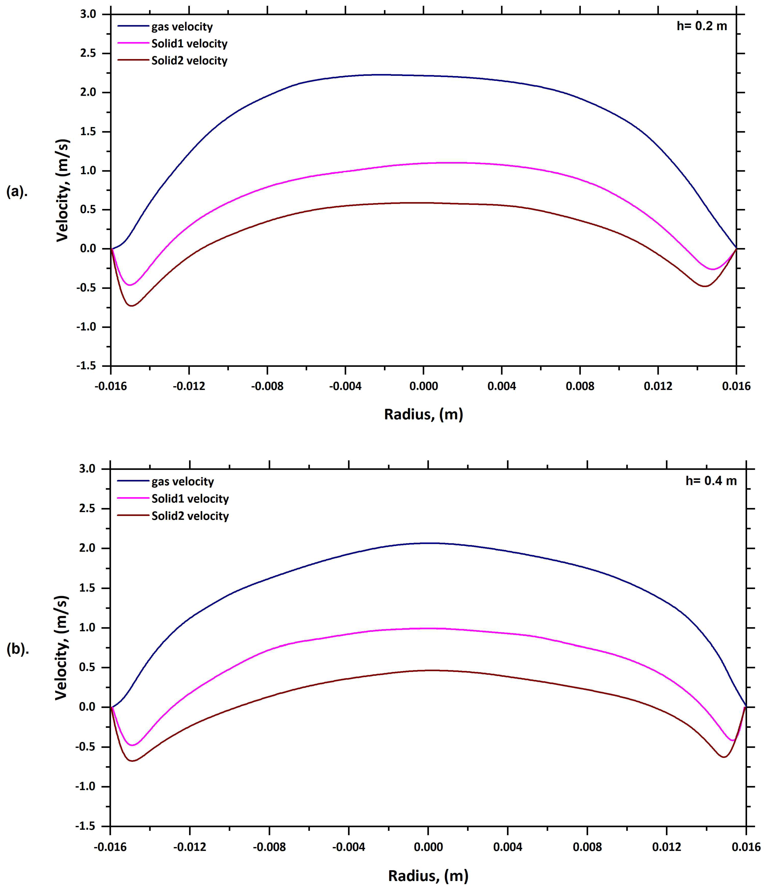
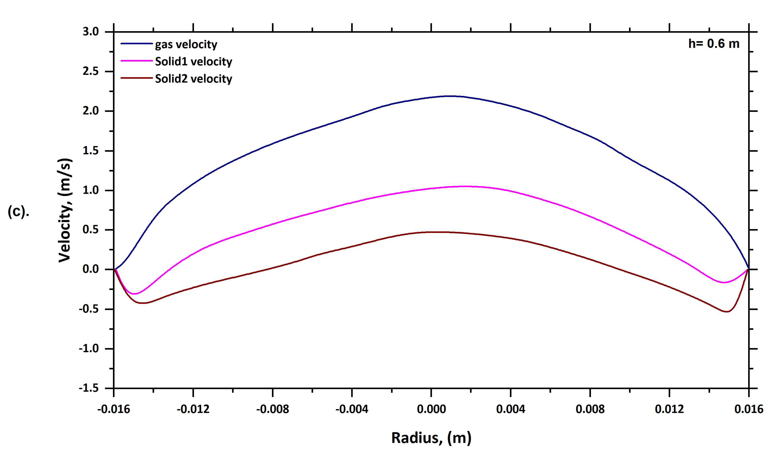
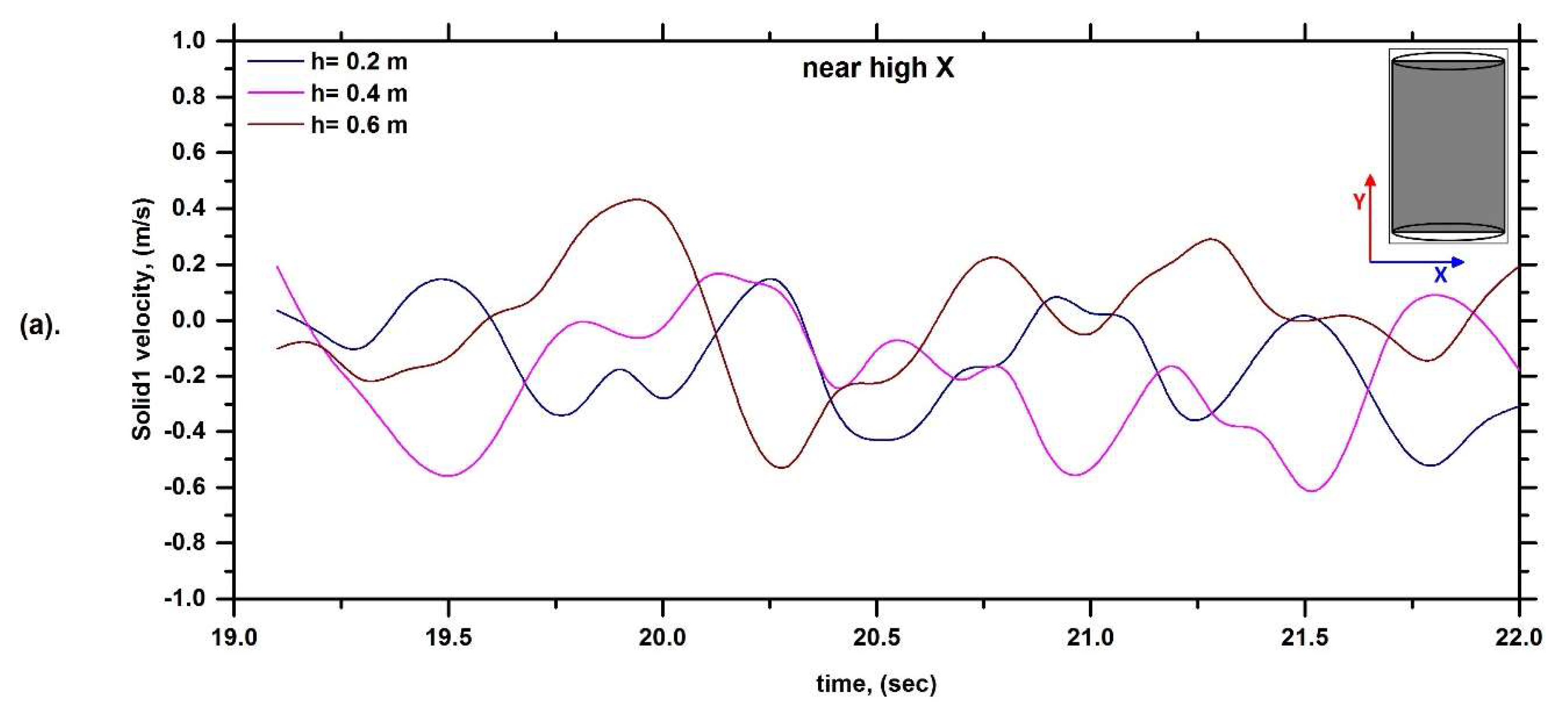
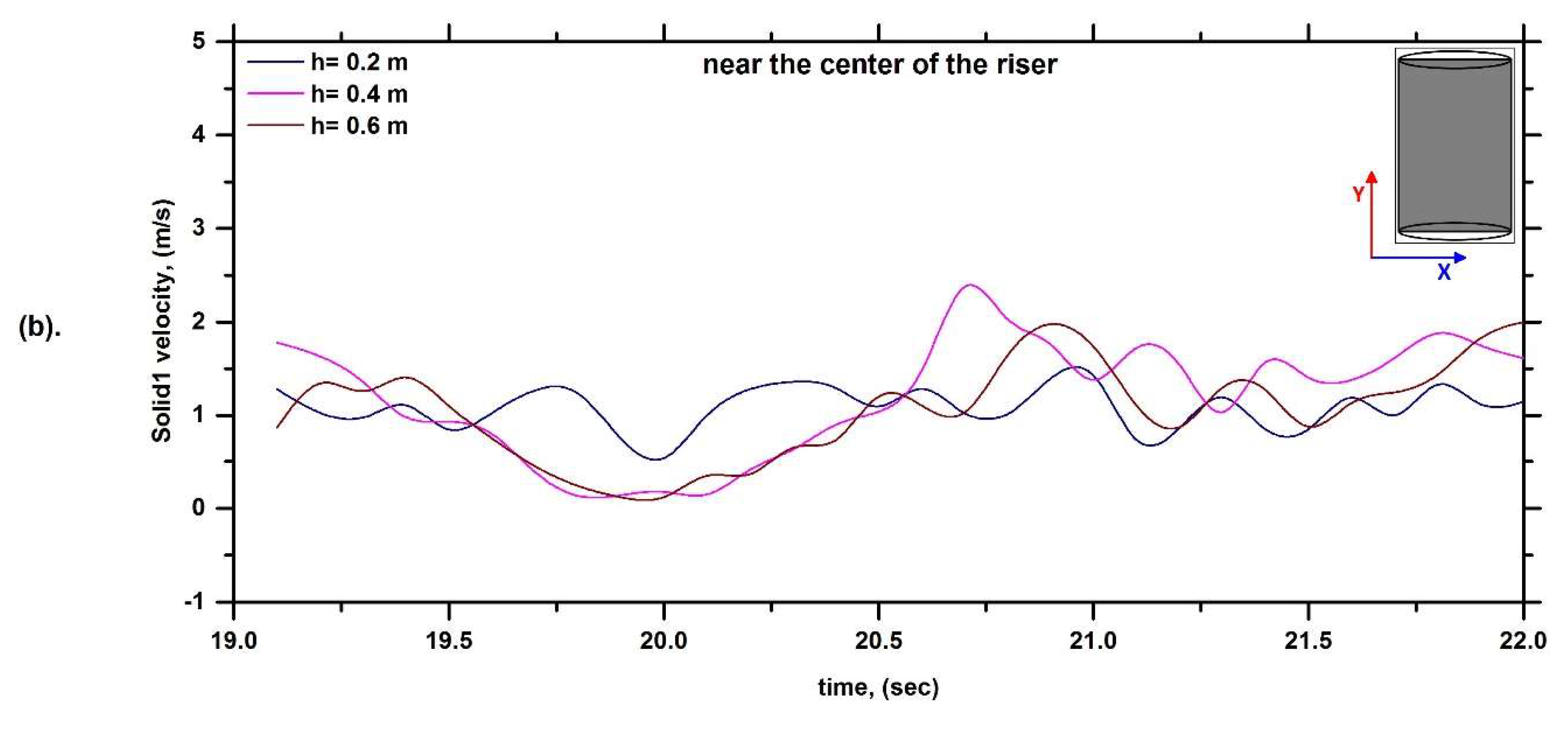
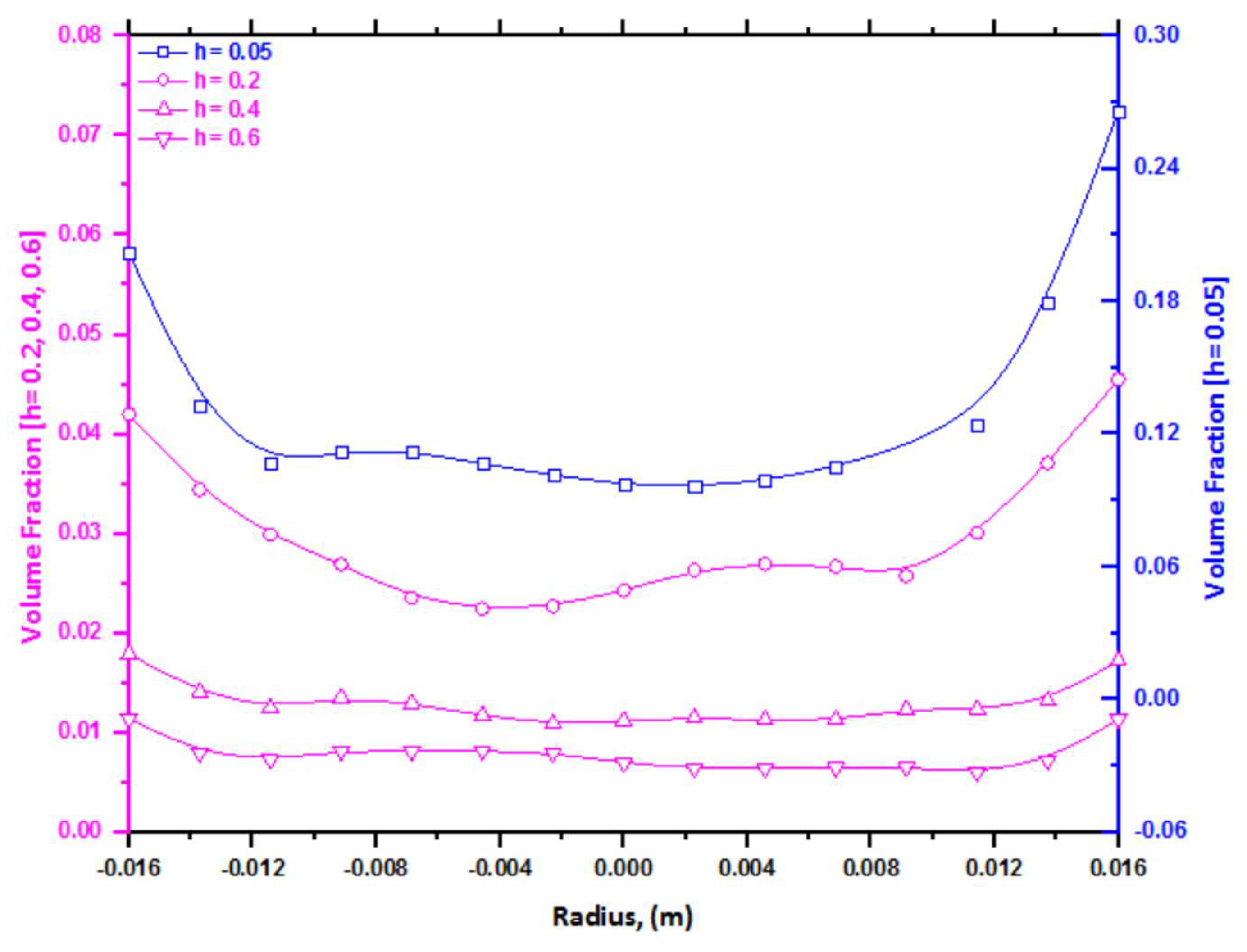
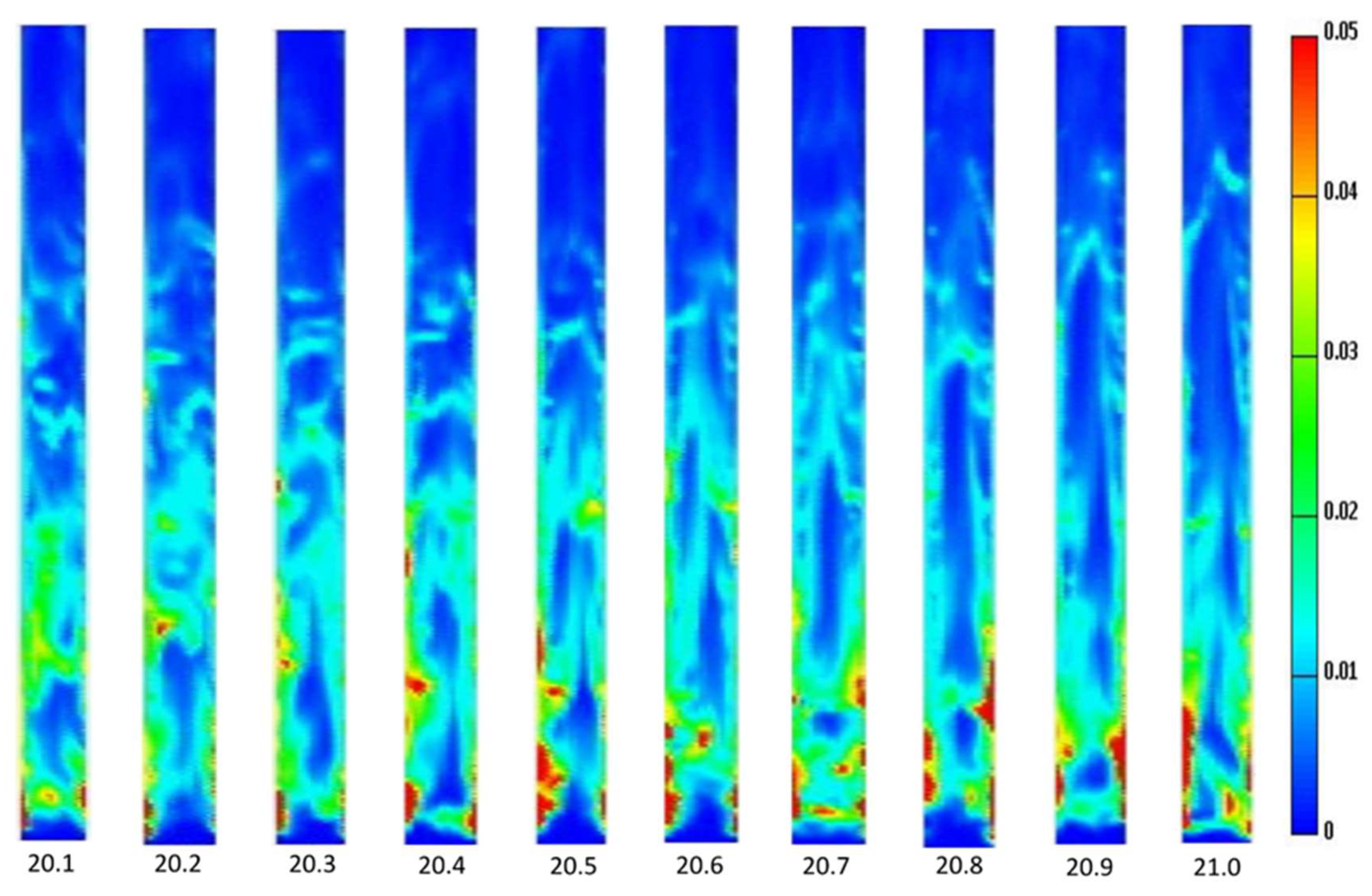
In this work, a new kinetic theory (KT) model for particles of different densities and sizes has been implemented in the commercial CFD software CFX and used to simulate the riser section of a circulating fluidised bed having particles of different sizes. Different flow properties for solid phases, such as solid viscosity, solid pressure, collisional heat flux and bulk viscosity resulting from particle–particle interactions, are obtained from the present CFD model. Interphase transfer terms (i.e., momentum transfer and fluctuating energy transfer) between the solid phases are also implemented into the CFD model through user-defined functions (UDFs). The k-ε turbulence model is used in simulating the circulating fluidised bed model. For verification, simulation results obtained with the new KT model are compared with experimental data, and then the model is used for further analysis. Using the CFD model, results were obtained for a three-dimensional circulating fluidised bed model that are in fairly good agreement with experimental results. The model successfully predicts typical CFB behaviour, such as
  • Core–annular flow in the riser,
  • Particle carryover,
  • Cluster formation,
  • Downward particle flow near the riser wall,
  • Relative velocity between particles of different sizes,
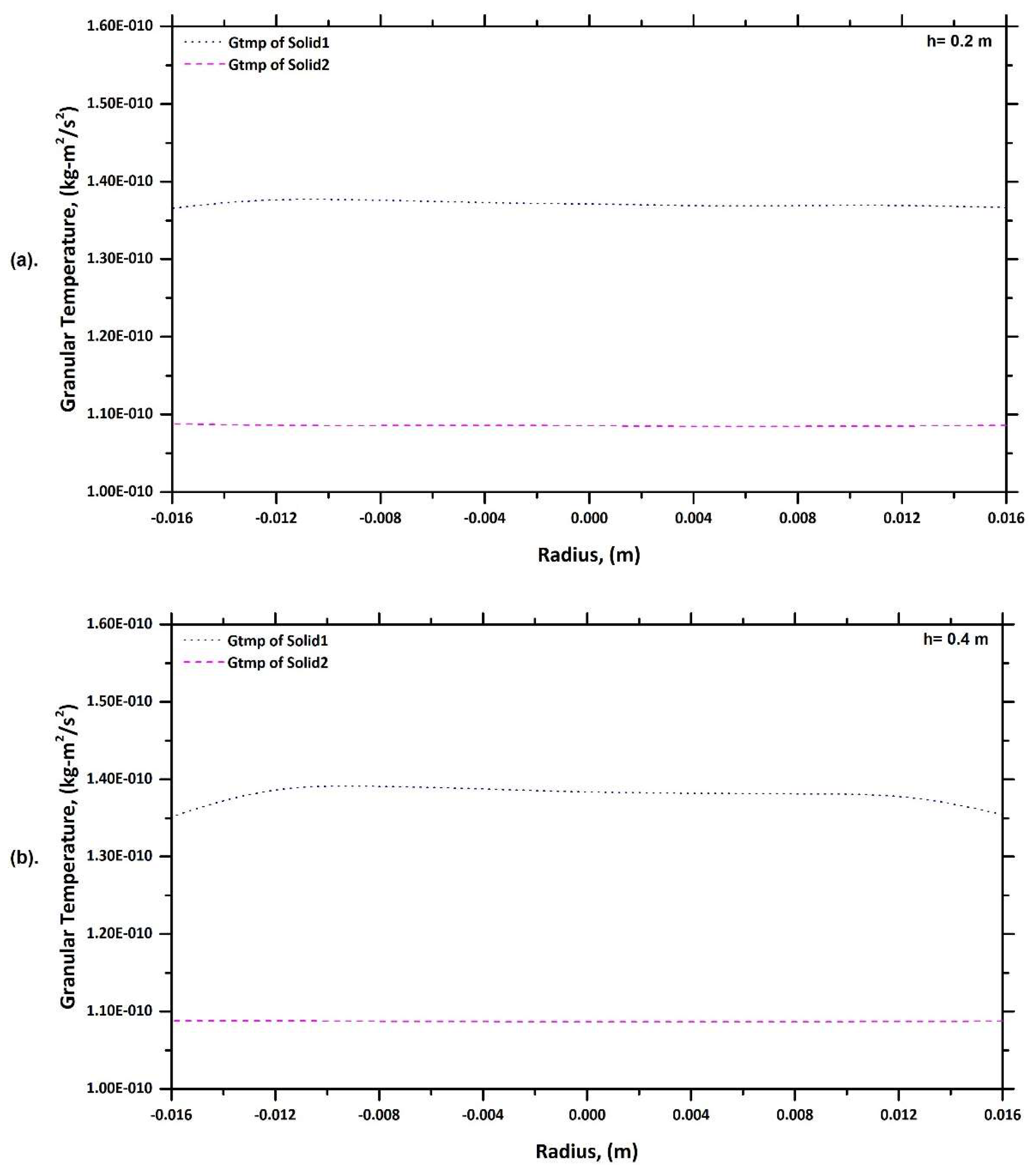
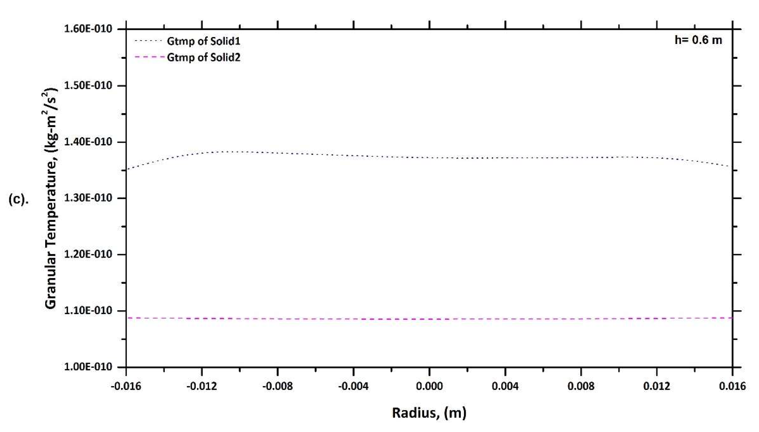
  • Different granular temperatures for particles of different sizes,
  • A turbulent bed of large diameter particles in the base of the riser and transport of the smaller particles well in the top section of the riser,
  • A higher concentration of solids in the wall region compared to the centre.
The predicted results are in qualitative agreement with published experimental work. This indicates that the multi-particle multiphase gas–solid flow model works fairly well.

Author Contributions

Methodology, F.R., A.A.R.S. and J.N.; Validation, F.R.; Writing—original draft, F.R.; Writing—review & editing, A.A.R.S.; Visualization, A.A.R.S.; Supervision, J.N. All authors have read and agreed to the published version of the manuscript.

Funding

This research received no external funding.

Data Availability Statement

The data supporting the findings of this study is available upon request.

Conflicts of Interest

The authors declare no conflict of interest.

Nomenclature

AParticle projected area
CdDrag coefficient
CgFluctuating velocity of gas
ciInstantaneous velocity of particle i
cijRelative velocity
cjInstantaneous velocity of particle j
CpFluctuating velocity of particles
dDiameter of particle
DwWest diffusion coefficient
eRestitution coefficient
FTotal external force
fiVelocity distribution of phase i
fjVelocity distribution of phase j
FpParticle drag force
GCombined velocity during collision
g Radial distributive function
hwDistance between west and central nodes
IUnit tensor
mimass of particle i
mjmass of particle j
mkmass of particle k
n Cell face normal vector
NNumber of phases
niNumber of particles in i phase
NijNumber of collisions between i and j particles
nNumber of particles
PParticle stress or pressure tensor
PPressure
PcCollisional stress tensor
PkKinetic stress tensor
Pk,iKinetic stress tensor of phase i
qcCollisional heat flux
qkKinetic heat flux
rPosition vector
Re Reynolds number
riRadius of particle i
RijSummation of the radius (ri + rj)
rjRadius of particle j
S Source term
tTime
viHydrodynamic mean velocity of i phase
vjHydrodynamic mean velocity of j phase
VpVolume of particle
xiArbitrary position of particle i.
xjArbitrary position of particle j.
Greek Symbols
η Kolmogorov length scale
θGranular temperature (old definition)
μsSolid viscosity
μcol,sCollisional part of solid viscosity
μkin,sKinetic part of solid viscosity
μdil,sDilute viscosity
εVolume fraction
ρDensity
τsShear stress
βgsDrag coefficient between gas and solid
ΓDiffusion coefficient
ωAngular velocity
ζiBulk viscosity of phase I

References

  1. Zhao, G.J.; Shi, X.G.; Wu, Y.Y.; Wang, M.; Zhang, M.X.; Gao, J.S.; Lan, X.Y. 3D CFD simulation of gas-solids hydrodynamics and bubbles behaviors in empty and packed bubbling fluidized beds. Powder Technol. 2019, 351, 1–15. [Google Scholar] [CrossRef]
  2. Luo, Z.; Zhao, Y.; Lv, B.; Fu, Y.; Xu, X.; Chen, C. Dry coal beneficiation technique in the gas–solid fluidized bed: A review. Int. J. Coal Prep. Util. 2019, 42, 1–29. [Google Scholar] [CrossRef]
  3. Rahaman, M.F.; Naser, J.; Witt, P.J. An unequal granular temperature kinetic theory: Description of granular flow with multiple particle classes. Powder Technol. 2003, 138, 82–92. [Google Scholar] [CrossRef]
  4. Lv, B.; Luo, Z.; Fu, Y.; Zhang, B.; Qin, X.; Zhu, X. Particle mixing behavior of fine coal in density control of gas–solid separation fluidized bed. Particuology 2019, 50, 76–87. [Google Scholar] [CrossRef]
  5. Fu, Z.; Zhu, J.; Barghi, S.; Zhao, Y.; Luo, Z.; Duan, C. The distribution of bed density in an air dense medium fluidized bed with single and binary mixtures of Geldart B and/or D particles. Miner. Eng. 2019, 142, 105926. [Google Scholar] [CrossRef]
  6. Ostermeier, P.; Vandersickel, A.; Gleis, S.; Spliethoff, H. Numerical Approaches for Modeling Gas–Solid Fluidized Bed Reactors: Comparison of Models and Application to Different Technical Problems. J. Energy Resour. Technol. 2019, 141, 070707. [Google Scholar] [CrossRef]
  7. Gidaspow, D.; Lu, H.L. Collisional viscosity of FCC particles in a CFB. Aiche J. 1996, 42, 2503–2510. [Google Scholar] [CrossRef]
  8. Ding, J.; Gidaspow, D. A Bubbling Fluidization Model Using Kinetic-Theory of Granular Flow. Aiche J. 1990, 36, 523–538. [Google Scholar] [CrossRef]
  9. Arastoopour, H.; Pakdel, P.; Adewumi, M. Hydrodynamic analysis of dilute gas—Solids flow in a vertical pipe. Powder Technol. 1990, 62, 163–170. [Google Scholar] [CrossRef]
  10. Peng, L.; Wu, Y.; Wang, C.; Gao, J.; Lan, X. 2.5D CFD simulations of gas–solids flow in cylindrical CFB risers. Powder Technol. 2016, 291, 229–243. [Google Scholar] [CrossRef]
  11. Zhou, Q.; Wang, J. CFD study of mixing and segregation in CFB risers: Extension of EMMS drag model to binary gas–solid flow. Chem. Eng. Sci. 2015, 122, 637–651. [Google Scholar] [CrossRef]
  12. Wang, S.; Liu, G.D.; Lu, H.L.; Sun, L.Y.; Xu, P.F. CFD simulation of bubbling fluidized beds using kinetic theory of rough sphere. Chem. Eng. Sci. 2012, 71, 185–201. [Google Scholar] [CrossRef]
  13. Lun, C.K.K.; Savage, S.B.; Jeffrey, D.J.; Chepurniy, N. Kinetic theories for granular flow: Inelastic particles in Couette flow and slightly inelastic particles in a general flowfield. J. Fluid Mech. 1984, 140, 223–256. [Google Scholar] [CrossRef]
  14. Jenkins, J.T.; Savage, S.B. A theory for the rapid flow of identical, smooth, nearly elastic, spherical particles. J. Fluid Mech. 1983, 130, 187–202. [Google Scholar] [CrossRef]
  15. Yang, L.; Padding, J.T.; Kuipers, J.A.M. Modification of kinetic theory of granular flow for frictional spheres, Part I: Two-fluid model derivation and numerical implementation. Chem. Eng. Sci. 2016, 152, 767–782. [Google Scholar] [CrossRef]
  16. Gidaspow, D. Multiphase Flow and Fluidization: Continuum and Kinetic Theory Descriptions; Academic Press: Cambridge, MA, USA, 2012. [Google Scholar]
  17. Manger, E. Modelling and Simulation of Gas/Solids Flow in Curvilinear Co ordinates. Ph.D. Thesis, Norwegian University of Science and Technology, Trondheim, Norway, 1996. [Google Scholar]
  18. Bell, R.A. Numerical Modelling of Multi-Particle Flows in Bubbling Gas-Solid Fluidized Beds; Swinburne University of Technology: Melbourne City, Australia, 2000. [Google Scholar]
  19. Huilin, L.; Wenti, L.; Rushan, B.; Lidan, Y.; Gidaspow, D. Kinetic theory of fluidized binary granular mixtures with unequal granular temperature. Phys. A Stat. Mech. Its Appl. 2000, 284, 265–276. [Google Scholar] [CrossRef]
  20. Mathiesen, V.; Solberg, T.; Hjertager, B.H. An experimental and computational study of multiphase flow behavior in a circulating fluidized bed. Int. J. Multiph. Flow 2000, 26, 387–419. [Google Scholar] [CrossRef]
  21. Dodds, D.; Sarhan, A.R.; Naser, J. CFD Investigation into the Effects of Surrounding Particle Location on the Drag Coefficient. Fluids 2022, 7, 331. [Google Scholar] [CrossRef]
  22. Weaver, D.S.; Mišković, S. An Analysis of CFD-DEM with Coarse Graining for Turbulent Particle-Laden Jet Flows. Fluids 2023, 8, 215. [Google Scholar] [CrossRef]
  23. Wang, S.; Luo, K.; Hu, C.S.; Sun, L.Y.; Fan, J.R. Effect of superficial gas velocity on solid behaviors in a full-loop CFB. Powder Technol. 2018, 333, 91–105. [Google Scholar] [CrossRef]
  24. Zhang, W.; You, C.F. Numerical simulation of particulate flows in CFB riser with drag corrections based on particle distribution characterization. Chem. Eng. J. 2016, 303, 145–155. [Google Scholar] [CrossRef]
  25. Wang, Q.; Niemi, T.; Peltola, J.; Kallio, S.; Yang, H.; Lu, J.; Wei, L. Particle size distribution in CPFD modeling of gas–solid flows in a CFB riser. Particuology 2015, 21, 107–117. [Google Scholar] [CrossRef]
  26. Rossbach, V.; Utzig, J.; Decker, R.K.; Noriler, D.; Meier, H.F. Numerical gas-solid flow analysis of ring-baffled risers. Powder Technol. 2016, 297, 320–329. [Google Scholar] [CrossRef]
  27. Wu, J.; Binbo, J.; Chen, J.; Yang, Y. Multi-scale study of particle flow in silos. Adv. Powder Technol. 2009, 20, 62–73. [Google Scholar] [CrossRef]
  28. Miin, C.S.; Sulaiman, S.A.; Raghavan, V.R.; Heikal, M.R.; Naz, M.Y. Hydrodynamics of multi-sized particles in stable regime of a swirling bed. Korean J. Chem. Eng. 2015, 32, 2361–2367. [Google Scholar] [CrossRef]
  29. Zheng, N.; Liu, H.; Fang, J.; Wei, J. Numerical investigation of bed-to-tube heat transfer in a shallow fluidized bed containing mixed-size particles. Int. J. Heat Mass Transf. 2023, 211, 124252. [Google Scholar] [CrossRef]
  30. Mathiesen, V. An Experimental and computational Study of Multiphase Flow Behavior in Circulating Fluidized Beds; Telemark Institute of Technology: Notodden, Norway, 1997. [Google Scholar]
  31. Rahaman, M.F.; Sarhan, A.R.; Naser, J. Kinetic theory for multi-particulate flow: Description of granular flow with rotary movement of particles. Powder Technol. 2020, 360, 780–788. [Google Scholar] [CrossRef]
  32. Abramov, R.V. Turbulence via Intermolecular Potential: Viscosity and Transition Range of the Reynolds Number. Fluids 2023, 8, 101. [Google Scholar] [CrossRef]
  33. Witt, P.J.; Perry, J.H.; Schwarz, M.P. A numerical model for predicting bubble formation in a 3D fluidized bed. Appl. Math. Model. 1998, 22, 1071–1080. [Google Scholar] [CrossRef]
  34. Van Wachem, B.G.M.; Schouten, J.C.; van den Bleek, C.M.; Krishna, R.; Sinclair, J.L. Comparative analysis of CFD models of dense gas–solid systems. Aiche J. 2001, 47, 1035–1051. [Google Scholar] [CrossRef]
  35. Tsuo, Y.P.; Gidaspow, D. Computation of Flow Patterns in Circulating Fluidized-Beds. Aiche J. 1990, 36, 885–896. [Google Scholar] [CrossRef]
  36. Sobieski, W. Drag Coefficient in Solid–Fluid System Modeling with the Eulerian Multiphase Model. Dry. Technol. 2011, 29, 111–125. [Google Scholar] [CrossRef]
  37. Zhang, Y.F.; Arastoopour, H. Dilute Fluidized Cracking Catalyst Particles—Gas-Flow Behavior in the Riser of a Circulating Fluidized-Bed. Powder Technol. 1995, 84, 221–229. [Google Scholar] [CrossRef]
  38. Miller, A.; Gidaspow, D. Dense, Vertical Gas-Solid Flow in a Pipe. Aiche J. 1992, 38, 1801–1815. [Google Scholar] [CrossRef]
  39. Farrell, M.; Lun, C.K.K.; Savage, S.B. A simple kinetic theory for granular flow of binary mixtures of smooth, inelastic, spherical particles. Acta Mech. 1986, 63, 45–60. [Google Scholar] [CrossRef]
  40. Jenkins, J.T.; Mancini, F. Balance Laws and Constitutive Relations for Plane Flows of a Dense, Binary Mixture of Smooth, Nearly Elastic, Circular Disks. J. Appl. Mech. T ASME 1987, 54, 27–34. [Google Scholar] [CrossRef]
Figure 1. A schematic sketch of the laboratory scale CFB Mathiesen [30].
Fluids 08 00257 g001
Figure 2. Grid independence test.
Fluids 08 00257 g002
Figure 3. Initial volume fractions in the riser of the simulated CFB.
Fluids 08 00257 g003
Figure 4. Instantaneous velocity vectors in the riser at t = 21.0 s.
Fluids 08 00257 g004
Figure 5. Velocity profiles at different height of the riser; (a) h = 0.2 m, (b) h = 0.4 m and (c) h = 0.6. m.
Fluids 08 00257 g005aFluids 08 00257 g005b
Figure 6. Influence of height on Solid1 velocity variation with time; (a) near high X, (b) near the centre of the riser and (c) near low X.
Fluids 08 00257 g006aFluids 08 00257 g006bFluids 08 00257 g006c
Figure 7. Influence of height on Solid2 velocity variation with time; (a) near high X, (b) near the centre of the riser and (c) near low X.
Fluids 08 00257 g007aFluids 08 00257 g007bFluids 08 00257 g007c
Figure 8. Simulated particle velocity profiles with proposed kinetic theory model [30].
Fluids 08 00257 g008
Figure 9. Simulated particle velocity profiles with previous kinetic theory model [30].
Fluids 08 00257 g009
Figure 10. Time-averaged solid volume fraction at different heights.
Fluids 08 00257 g010
Figure 11. Solid1 volume fraction distribution in the riser (time = 20.1–21.0 s).
Fluids 08 00257 g011
Figure 12. Solid2 volume fraction distribution in the riser (time = 20.1–21.0 s).
Fluids 08 00257 g012
Figure 13. Influence of height on Solid1 volume fraction variation with time; (a) near high X, (b) near the centre of the riser and (c) near low X.
Fluids 08 00257 g013aFluids 08 00257 g013b
Figure 14. Influence of height on Solid2 volume fraction variation with time; (a) near high X, (b) near the centre of the riser and (c) near low X.
Fluids 08 00257 g014aFluids 08 00257 g014b
Figure 15. Time-average granular temperature profile at different heights of the riser; (a) h = 0.2 m, (b) h = 0.4 m and (c) h = 0.6. m.
Fluids 08 00257 g015aFluids 08 00257 g015b
Table 1. Governing equations for gas–solid flow through riser, constitutive law and boundary conditions.
1. The number of binary collisions
N i j = π 4 d i j 2 n i n j g i j ( m i m j θ i θ j ) 3 2 × 1 A 3 / 2 D 2 [ 1 + 3 π B 2 A D + 45 π B 4 8 ( A D ) 2 ]
were coefficients A, B, D:
A = m i θ j + m j θ i 2 θ i θ j B = m i m j ( θ i θ j ) 2 m 0 θ i θ j D = m i m j ( m i θ i + m j θ j ) 2 m 0 2 θ i θ j
2. The conservation equations
n ψ i t + . ( n i < c i ψ i > + j P c , i j ) = < n i F i ψ i c > + N c , i j
Collisional stress contribution:
P c , i j = 1 2 d i j 3 c i j . k > 0 ( ψ i ψ i ) c i j . k k f i j ( 2 ) ( r 1 2 d i j k , c i , r + 1 2 d i j k , c j ) d k d c i d c j
N c , i j = 1 2 d i j 2 c i j . k > 0 ( ψ j + ψ i ψ j ψ i ) c i j . k f i j ( 2 ) ( r 1 2 d i j k , c i , r , c j ) d k d c i d c j
Conservation of mass for species i:
t ( n i m i ) + . ( n i m i v i ) = 0
Volume fraction of species i:
ε i = n i m i ρ i
Conservation of momentum of species i:
t ( ε i ρ i v i ) + . ( ε i ρ i v i v i ) = . ( P k , i + P c , i ) + ε i ρ i F i + N M , i
Conservation equation for the fluctuating translational energy for species i:
9 π d i 3 [ t ( ε i θ i ) + . ( ε i θ i v i ) ] = ( P k , i + P c , i ) : v i ( q k , i + q c , i ) + ε i ρ i F i C i + N E , i
3. Constitutive relations
Pressure tensor
P k , ij = ρ i θ i m i I + 4 μ s , d i l ( 1 + e i j ) g o ( 1 + 4 5 ε s , i g i j ( 1 + e i j ) ) s v i
Solid phase pressure
P si = ρ i θ i m i + j π 48 ( 1 + e i j ) d i j 3 g i j m i m j n i n j m o ( m i m j θ i θ j ) 3 2 1 A 3 / 2 D 5 / 2 [ 1 + 15 π B 2 4 A D + ]
Solid shear viscosity
μ i = j { 2 μ i , d i l ( 1 + e i j ) g i j ( 1 + 4 5 ε s , i g i j ( 1 + e i j ) ) ( 1 + 4 π 15 d i j 3 n j g i j m i m o ( 1 + e i j ) ) + π 240 θ i g i j d i j 4 ( m i m j m o ) 2 ( 1 + e i j ) n i n j ( m i m j θ i θ j ) 3 / 2 S 1 }
Dilute viscosity
μ i , d i l = 24 ε s i θ i ρ i π 2 d i 3 m i j N i j
Energy dissipation
N E , i = j ( γ i j 1 + γ i j 2 )
Table 2. Numerical flow parameters used in this work.
Riser Dimensions-CylindricalDiameter0.032 m
Height1.0 m
Operating conditionsGas phaseρg = 1.2 kg m−3, μg = 0.00001 Pa s
Solid Phase IρsI = 2400 kg m−3, dI = 120 μm
Solid Phase IIρsII = 2400 kg m−3, dII = 185 μm
Initial bed height0.04 m
PressureAtmospheric pressure
Inlet gas velocityJg = 1.2 m s−1
Fraction of solids0.63
Table 3. Grids statistics.
PropertyMinimumMaximumAverage
Volume1.878 × 10−85.565 × 10−83.499 × 10−8
Skew0.91.00.9752
Twist1.01.01.0
Taper0.75881.00.8597
Stretch0.63621.00.8585
Table 4. Grids information.
BlockNINJNKNCell
1642004800
2642004800
3642004800
4442003200
5642004800
Total number of grid cells22,400
Table 5. Summary of the model formulation.
Commercial SoftwareCFX
GeneralLinear solver typeGSTB
Pressure formulationSIMPLE
Run modeUnsteady, ∆t = 0.001 s
Total time32.5 h
Gravitational body forceFull body force–Y direction
Convergence criteria0.0001
Mesh type22,400 grids, symmetric grid
ModelsThe Eulerian–Eulerian flow approach using Reynold’s Averaged Navier Stocks (RANS) and continuity Equations
Drag modelSchiller–Neumann Equation for particles [36].
Turbulence modelViscous-standard k–ε, dispersed
ControlNumber of phases = 2
Continuous phase = solid
Secondary phase = gas
Minimum volume fraction1 × 10−6
Boundary conditionsInlet conditionNormal velocity, 10% mean kinetic energy for k.
Outlet conditionStatic pressure, 100,000 Pa, zero gradient for k-ε.
Wall conditionNo slip conditions
Disclaimer/Publisher’s Note: The statements, opinions and data contained in all publications are solely those of the individual author(s) and contributor(s) and not of MDPI and/or the editor(s). MDPI and/or the editor(s) disclaim responsibility for any injury to people or property resulting from any ideas, methods, instructions or products referred to in the content.

