
Experimental Detection of Organised Motion in Complex Flows with Modified Spectral Proper Orthogonal Decomposition

Abstract
:1. Introduction
2. Spectral Proper Orthogonal Decomposition
2.1. Background
2.2. Computational Algorithms for SPOD
3. Experimental Approach
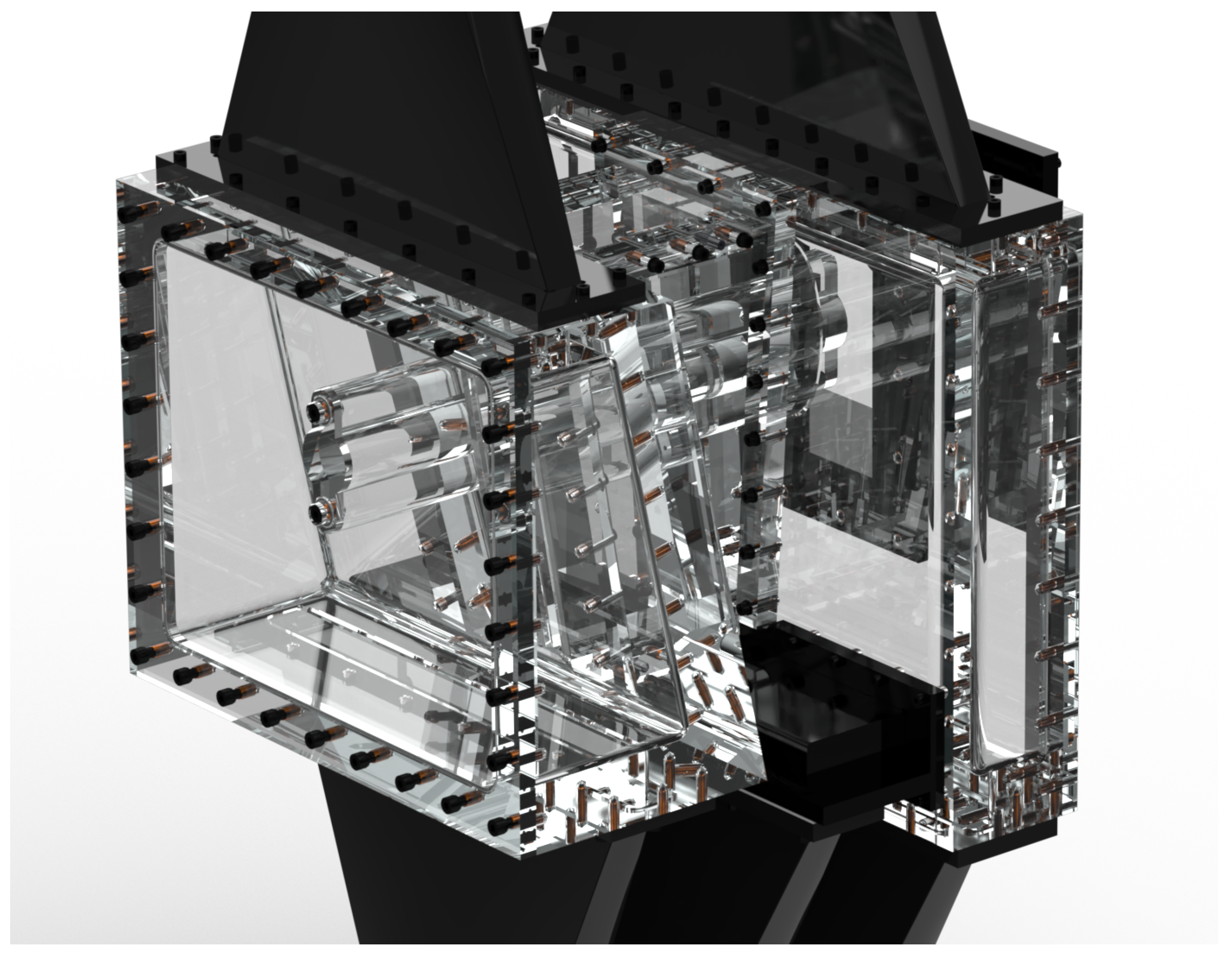
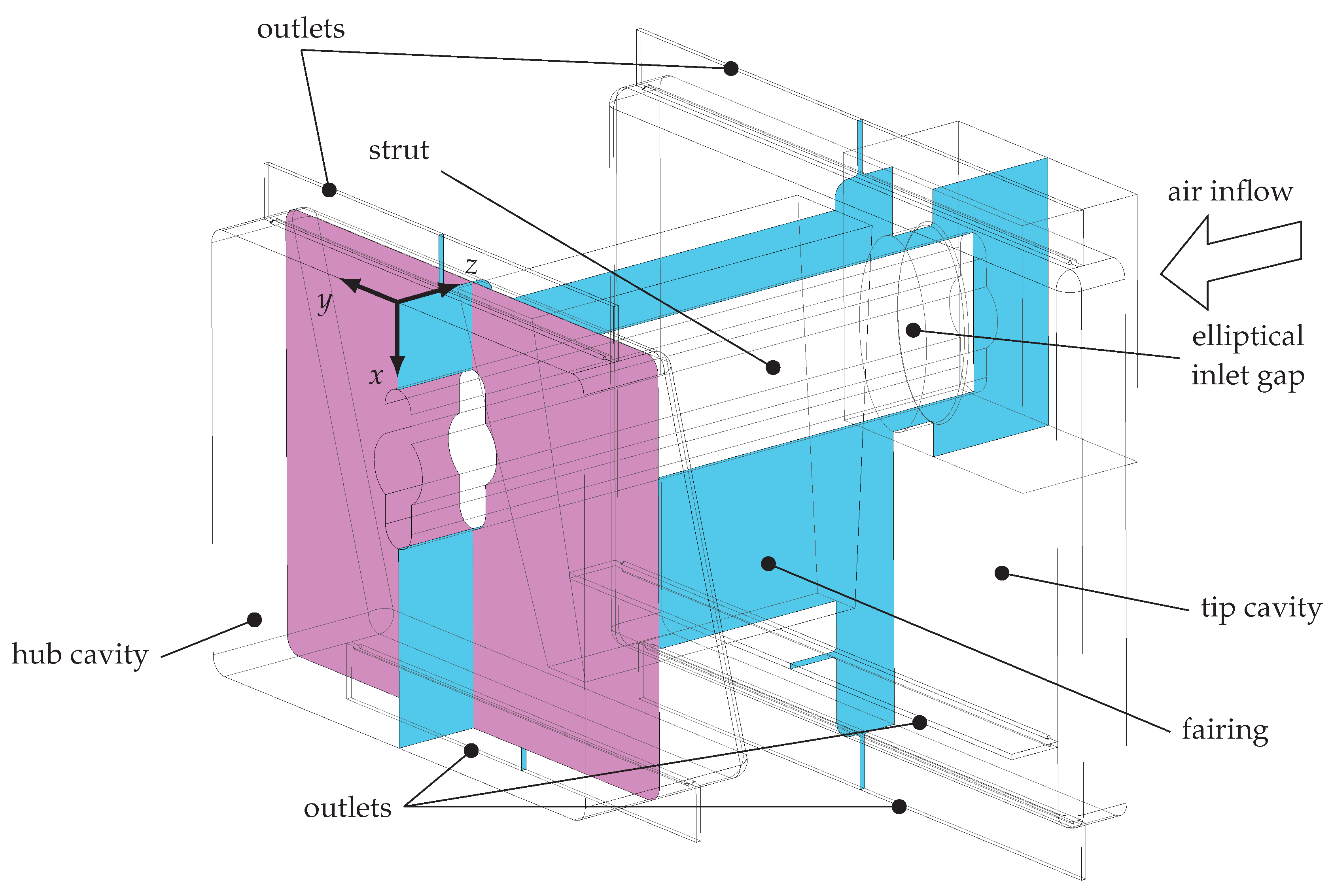
3.1. TCF Model
3.2. Measuring Equipment
4. Initial Analysis
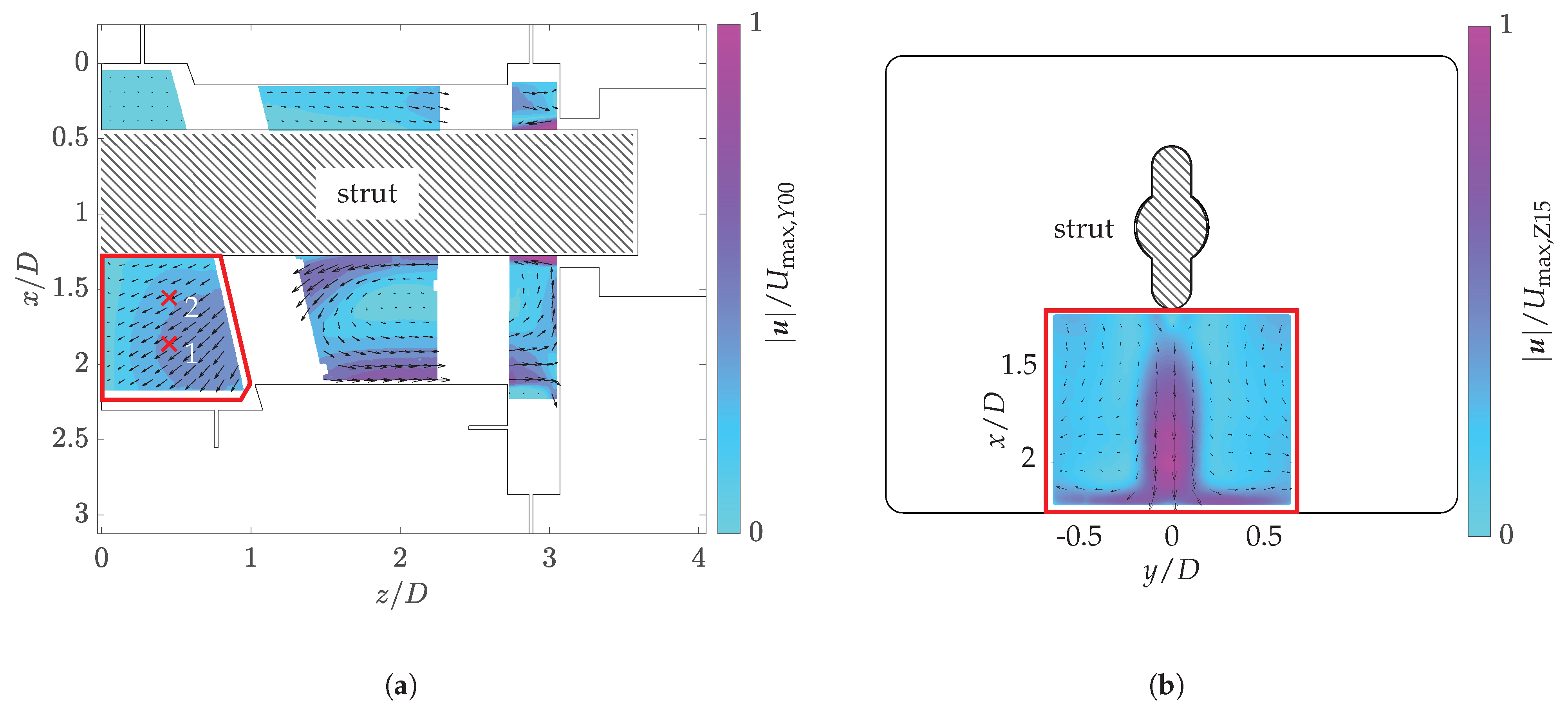
4.1. Mean Flow
4.2. Hot Wire Anemometry
5. Conventional SPOD
5.1. Data Acquisition
5.2. Evaluation
6. S2POD
6.1. Establishing Ideas
6.2. Results
7. Concluding Remarks
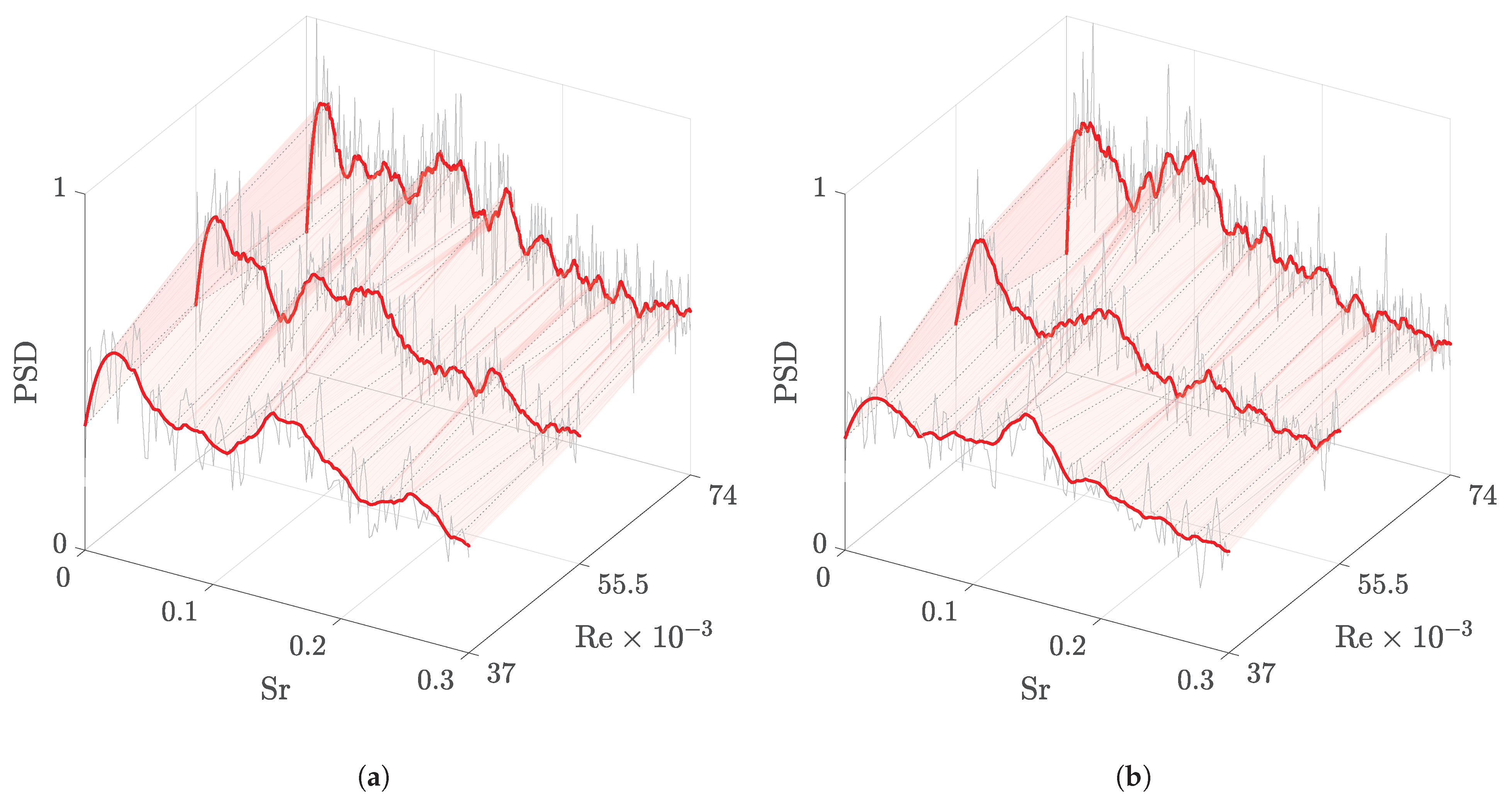
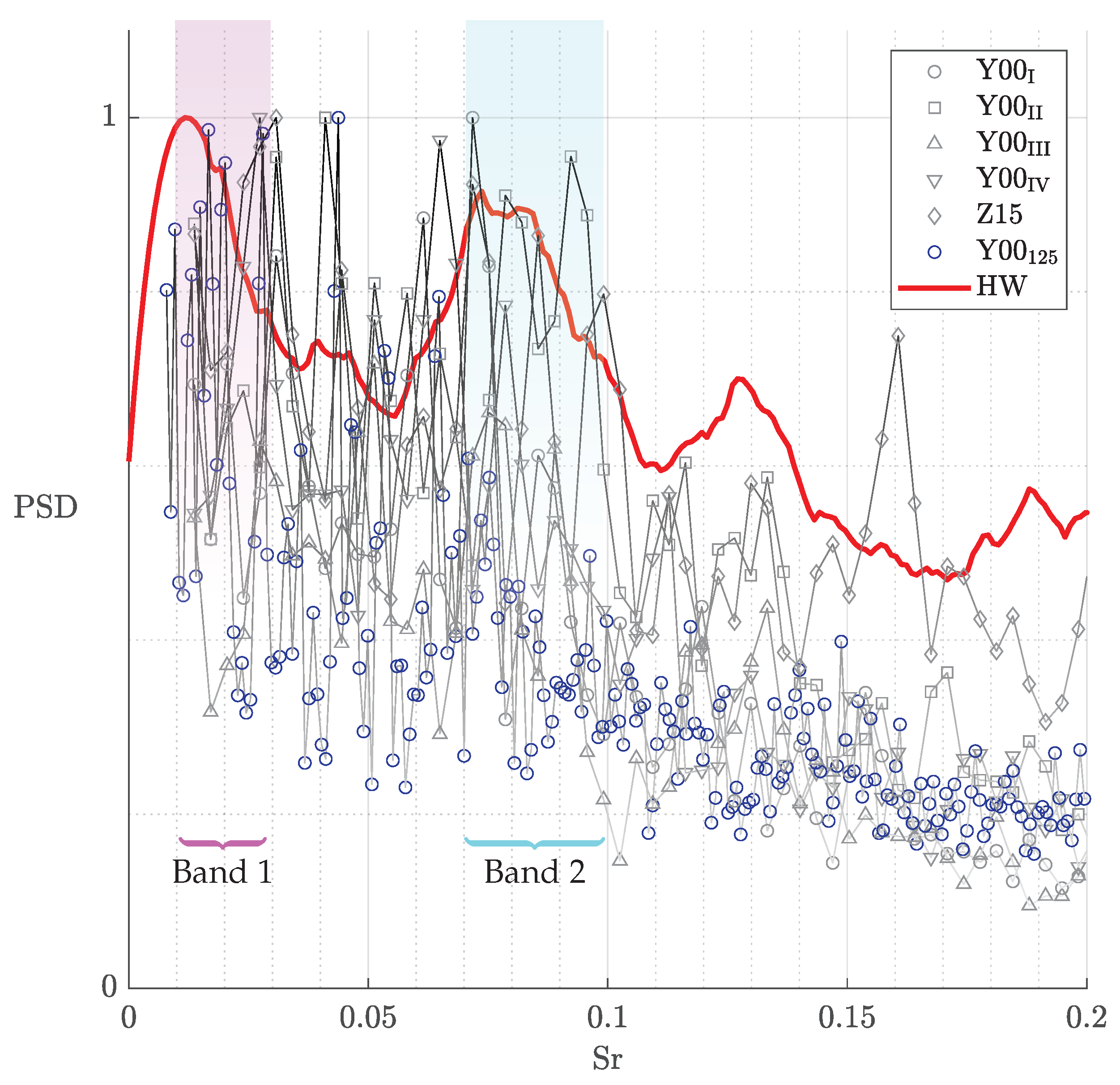
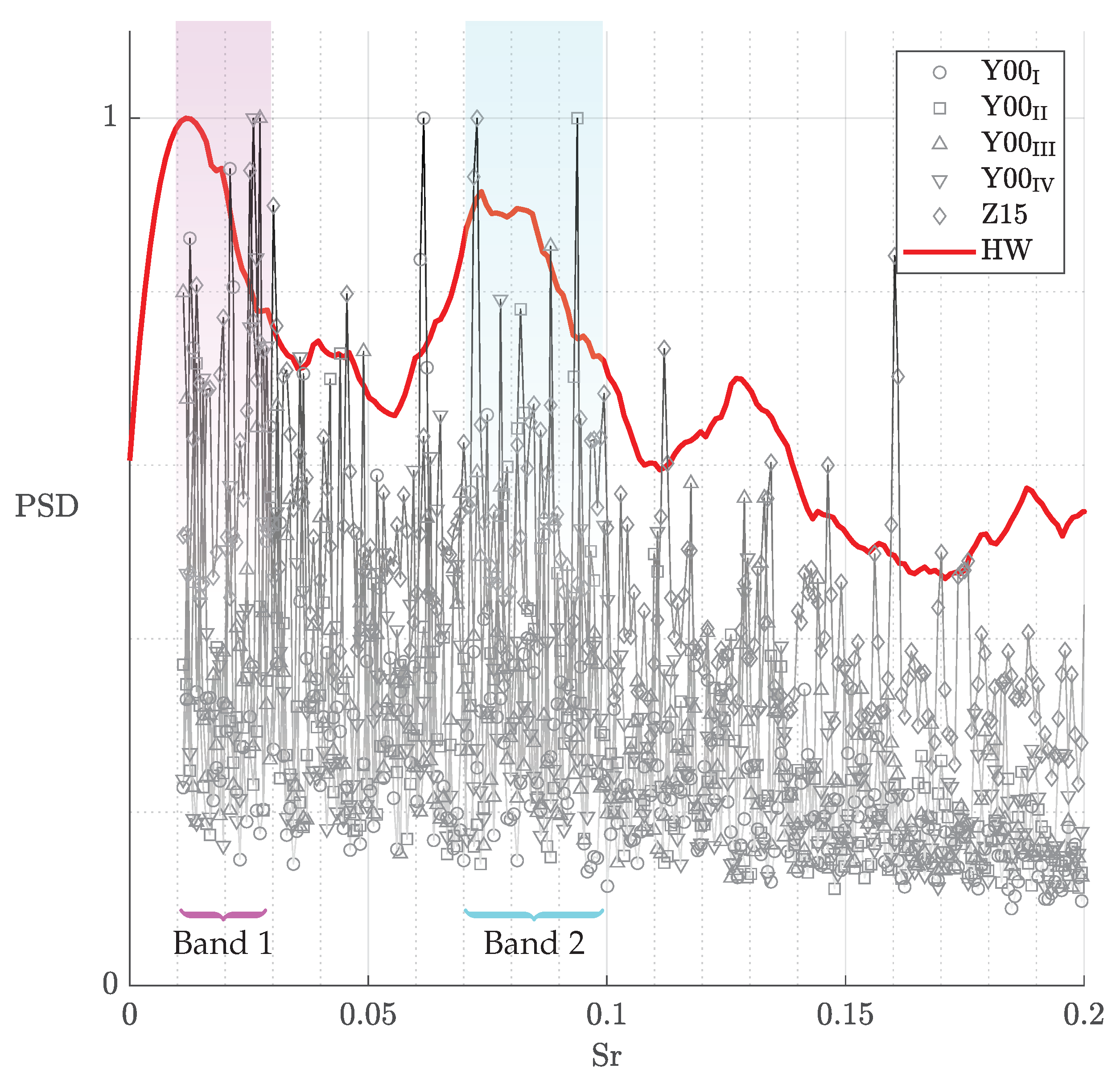
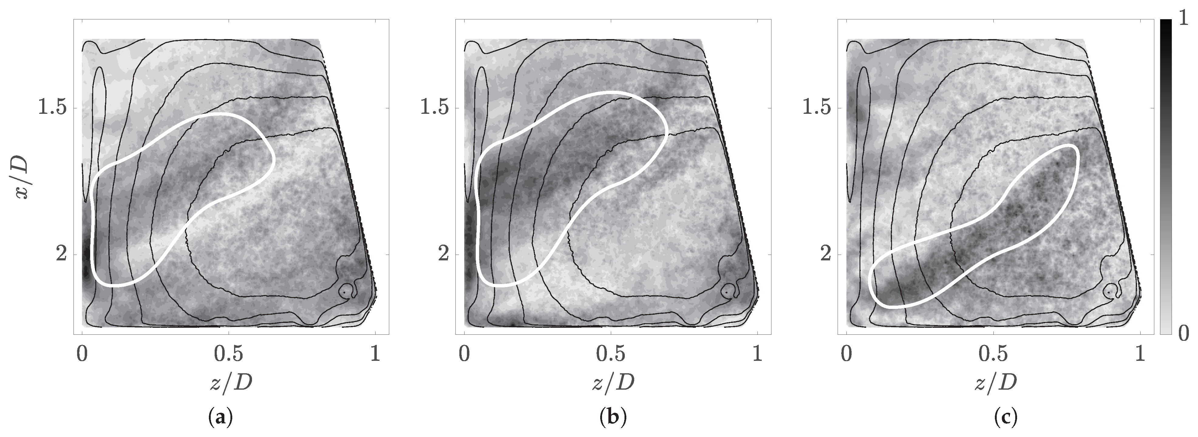
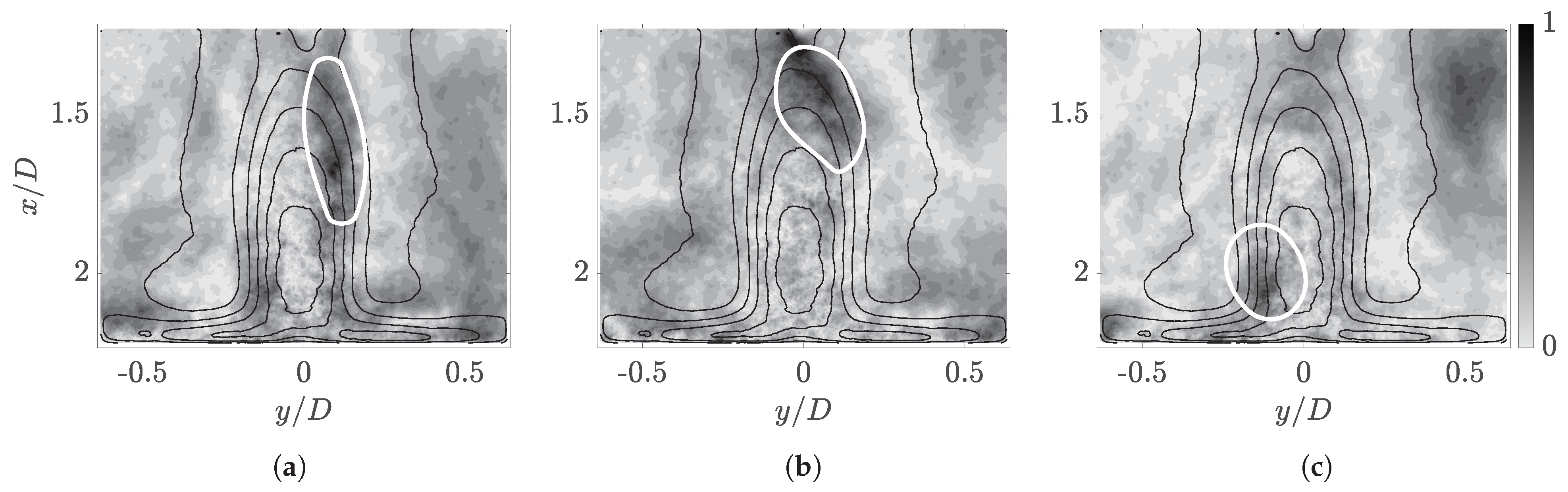
- A precessing structure in the shear layer surrounding the hub cavity jet, characterised by counterclockwise motion at several peaks between and .
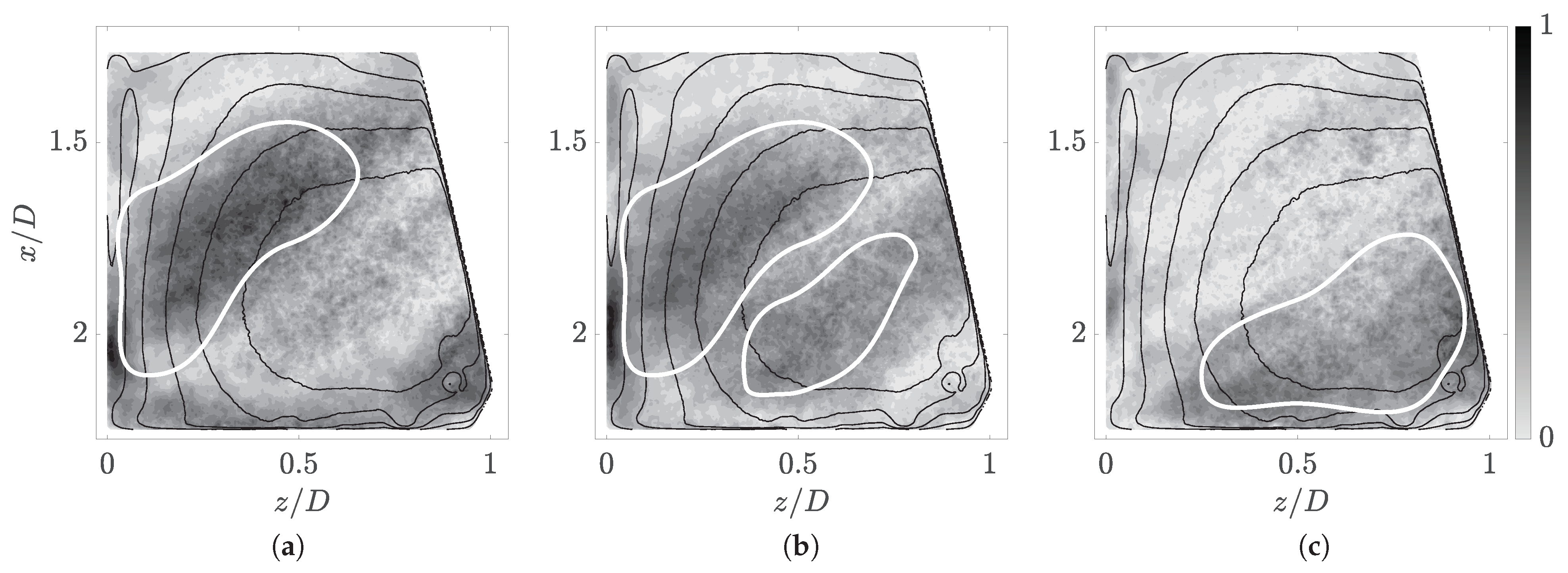
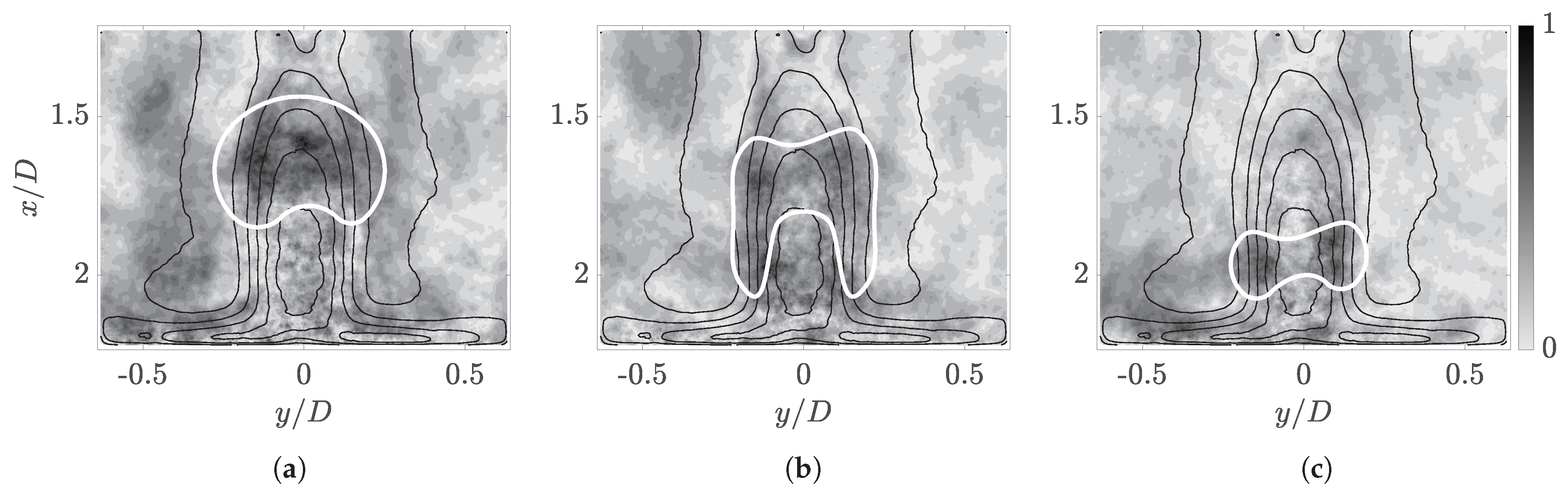
- A modulation of the jet’s flow speed at several peaks between and .
Author Contributions
Funding
Data Availability Statement
Acknowledgments
Conflicts of Interest
Abbreviations
| DFT | Discrete Fourier transform |
| FFT | Fast Fourier transform |
| FOV | Field of view |
| (HS)PIV | (High-speed) particle imagine velocimetry |
| K-L | Karhunen–Loève |
| PSD | Power spectral density |
| SGF | Savitzky–Golay finite impulse response filter |
| (S2)POD | (Spectral subsampling) proper orthogonal decomposition |
| TCF | Turbine centre frame |
| Latin Symbols | |
| Subsampling factor (-) | |
| d | Diameter () |
| D | Major axis of elliptical inflow slit () |
| f | Frequency () |
| Hilbert space (-) | |
| n | Natural number, No. of data points (-) |
| N | No. of spatial points (-) |
| Vector function (-) | |
| Correlation tensor (-) | |
| Reynolds number (-) | |
| Cross-spectral density tensor (-) | |
| Strouhal number (-) | |
| t | Time () |
| T | Period, measurement duration () |
| Cartesian velocity vector () | |
| U | Reference flow speed () |
| Input data array (-) | |
| V | Control volume/spatial domain (-) |
| Weight tensor (-) | |
| Spatial coordinates () | |
| x, y, z | Cartesian coordinates () |
| Fourier coefficient matrix (-) | |
| Set of independent variables (-) | |
| Greek Symbols | |
| Kronecker delta (-) | |
| Delta operator or difference (-) | |
| Eigenvalue (-) | |
| Eigenvalue matrix (-) | |
| Stochastic variable (-) | |
| Time shift () | |
| Phase () | |
| Eigenfunction (-) | |
| Eigenfunction matrix (-) | |
| Spectral eigenfunction (-) | |
| Spectral eigenfunction matrix (-) | |
| Variable domain (-) | |
| Subscripts | |
| 0 | Nominal, initial |
| ∞ | Far-field condition |
| Block | |
| f | Frequency index |
| No. of data points used in FFT | |
| Hydraulic diameter | |
| Local hot wire coordinate system | |
| Maximum occurring value | |
| Nyquist | |
| Sampling | |
| t | Time steps |
| x | Related to x-axis |
| y | Related to y-axis |
| Operators | |
| Expectation operator (-) | |
| Expectation value | |
| Fourier-transformed | |
| Conjugate transpose, effective | |
| Inner product |
References
- Sirovich, L. Turbulence and the dynamics of coherent structures. I–III. Q. Appl. Math. 1987, 45, 561–590. [Google Scholar] [CrossRef] [Green Version]
- Wang, Y.; Yu, B.; Wu, X.; Wei, J.J.; Li, F.C.; Kawaguchi, Y. POD study on the mechanism of turbulent drag reduction and heat transfer reduction based on Direct Numerical Simulation. Prog. Comput. Fluid Dyn. 2011, 11, 149–159. [Google Scholar] [CrossRef]
- Wang, Y.; Yu, B.; Wu, X.; Wang, P.; Li, F.C.; Kawaguchi, Y. POD Study on Large-Scale Structures of Viscoelastic Turbulent Drag-Reducing Flow. Adv. Mech. Eng. 2014, 6, 574381. [Google Scholar] [CrossRef]
- Schmid, P.J. Dynamic mode decomposition of numerical and experimental data. J. Fluid Mech. 2010, 656, 5–28. [Google Scholar] [CrossRef] [Green Version]
- Wynn, A.; Pearson, D.S.; Ganapathisubramani, B.; Goulart, P.J. Optimal mode decomposition for unsteady flows. J. Fluid Mech. 2013, 733, 473–503. [Google Scholar] [CrossRef] [Green Version]
- Farge, M. Wavelet transforms and their applications to turbulence. Annu. Rev. Fluid Mech. 1992, 24, 395–457. [Google Scholar] [CrossRef]
- Wang, Y.; Yu, B.; Wu, X.; Wang, P. POD and wavelet analyses on the flow structures of a polymer drag-reducing flow based on DNS data. Int. J. Heat Mass Transf. 2012, 55, 4849–4861. [Google Scholar] [CrossRef]
- Carassale, L. Analysis of aerodynamic pressure measurements by dynamic coherent structures. Probabilist. Eng. Mech. 2012, 28, 66–74. [Google Scholar] [CrossRef]
- Wu, T.; He, G. Independent component analysis of streamwise velocity fluctuations in turbulent channel flows. Theor. Appl. Mech. Lett. 2022, 12, 100349. [Google Scholar] [CrossRef]
- Towne, A.; Schmidt, O.T.; Colonius, T. Spectral proper orthogonal decomposition and its relationship to dynamic mode decomposition and resolvent analysis. J. Fluid Mech. 2018, 847, 821–867. [Google Scholar] [CrossRef] [Green Version]
- Schmidt, O.T.; Towne, A.; Rigas, G.; Colonius, T.; Brès, G.A. Spectral analysis of jet turbulence. J. Fluid Mech. 2018, 855, 953–982. [Google Scholar] [CrossRef] [Green Version]
- Araya, D.; Colonius, T.; Dabiri, J. Transition to bluff-body dynamics in the wake of vertical-axis wind turbines. J. Fluid Mech. 2017, 813, 346–381. [Google Scholar] [CrossRef] [Green Version]
- Lumley, J.L. The structure of inhomogeneous turbulent flows. In Atmospheric Turbulence and Radio Propagation; Yaglom, A.M., Tatarski, V.I., Eds.; Nauka: Moscow, Russia, 1967; pp. 166–178. [Google Scholar]
- Lumley, J.L. Stochastic Tools in Turbulence; Academic Press: New York, NY, USA, 2007. [Google Scholar]
- Picard, C.; Delville, J. Pressure velocity coupling in a subsonic round jet. Int. J. Heat Fluid Flow 2000, 21, 359–364. [Google Scholar] [CrossRef]
- Schmidt, O.T.; Colonius, T. Guide to Spectral Proper Orthogonal Decomposition. AIAA J. 2020, 58, 1023–1033. [Google Scholar] [CrossRef]
- Sieber, M.; Paschereit, O.C.; Oberleithner, K. Spectral proper orthogonal decomposition. J. Fluid Mech. 2016, 792, 798–828. [Google Scholar] [CrossRef] [Green Version]
- Aubry, N. On the hidden beauty of the proper orthogonal decomposition. Theor. Comput. Fluid Dyn. 1991, 2, 339–352. [Google Scholar] [CrossRef]
- Schmidt, O.T.; Towne, A. An efficient streaming algorithm for spectral proper orthogonal decomposition. Comput. Phys. Commun. 2018, 237, 98–109. [Google Scholar] [CrossRef] [Green Version]
- Schmidt, O.T. Spectral Proper Orthogonal Decomposition in Matlab. 2018. Available online: https://github.com/SpectralPOD/spod_matlab (accessed on 13 January 2022).
- Welch, P. The use of fast Fourier transform for the estimation of power spectra: A method based on time averaging over short, modified periodograms. IEEE Trans. Audio Electroacoust. 1967, 15, 70–73. [Google Scholar] [CrossRef] [Green Version]
- Köhler, S.; Stotz, S.; Schweikert, J.; Wolf, H.; Storm, P.; von Wolfersdorf, J. Aerodynamic study of flow phenomena in a turbine center frame. In Proceedings of the GPPS Chania22, Chania, Greece, 12–14 September 2022. [Google Scholar]
- Raffel, M.; Willert, C.E.; Scarano, F.; Kähler, C.J.; Wereley, S.T.; Kompenhans, J. Particle Image Velocimetry: A Pratical Guide, 3rd ed.; Springer: Berlin, Germany, 2018. [Google Scholar]
- Savitzky, A.; Golay, M.J.E. Smoothing and Differentiation of Data by Simplified Least Squares Procedures. Anal. Chem. 1964, 36, 1627–1639. [Google Scholar] [CrossRef]
- Orfanidis, S.J. Introduction to Signal Processing. 2010. Available online: https://www.ece.rutgers.edu/~orfanidi/intro2sp/ (accessed on 10 July 2022).
- Nakabayashi, T. Solving 2D Navier-Stokes Equations with SMAC Method. 2020. Available online: https://github.com/taku31/NavierStokes2D-with-SMAC-method (accessed on 8 October 2021).
- Bardera-Mora, R.; Barcala-Montejano, M.A.; Rodríguez-Sevillano, A.A.; de Sotto, M.R.; de Diego, G.G. Frequency prediction of a Von Karman vortex street based on a spectral analysis estimation. Am. J. Sci. Technol. 2018, 5, 26–34. [Google Scholar]
- Schlichting, H.; Gersten, K. Boundary-Layer Theory, 9th ed.; Springer: Berlin, Germany, 2017. [Google Scholar]
- Cafiero, G.; Ceglia, G.; Discetti, S.; Ianiro, A.; Astarita, T.; Cardone, G. On the three-dimensional precessing jet flow past a sudden expansion. Exp. Fluids 2014, 55, 1677. [Google Scholar] [CrossRef]


Disclaimer/Publisher’s Note: The statements, opinions and data contained in all publications are solely those of the individual author(s) and contributor(s) and not of MDPI and/or the editor(s). MDPI and/or the editor(s) disclaim responsibility for any injury to people or property resulting from any ideas, methods, instructions or products referred to in the content. |
© 2023 by the authors. Licensee MDPI, Basel, Switzerland. This article is an open access article distributed under the terms and conditions of the Creative Commons Attribution (CC BY) license (https://creativecommons.org/licenses/by/4.0/).
Share and Cite
Schneider, N.; Köhler, S.; von Wolfersdorf, J. Experimental Detection of Organised Motion in Complex Flows with Modified Spectral Proper Orthogonal Decomposition. Fluids 2023, 8, 184. https://doi.org/10.3390/fluids8060184
Schneider N, Köhler S, von Wolfersdorf J. Experimental Detection of Organised Motion in Complex Flows with Modified Spectral Proper Orthogonal Decomposition. Fluids. 2023; 8(6):184. https://doi.org/10.3390/fluids8060184
Chicago/Turabian StyleSchneider, Nick, Simon Köhler, and Jens von Wolfersdorf. 2023. "Experimental Detection of Organised Motion in Complex Flows with Modified Spectral Proper Orthogonal Decomposition" Fluids 8, no. 6: 184. https://doi.org/10.3390/fluids8060184