Author Contributions
Conceptualization, J.A.; methodology, J.A.; software, H.M.A.H. and Y.S.; formal analysis, Y.S.; investigation, H.M.A.H. and Y.S.; resources, J.A.; writing—original draft preparation, H.M.A.H. and Y.S.; writing—review and editing, J.A. and Y.S.; visualization, Y.S.; supervision, J.A.; project administration, J.A. All authors have read and agreed to the published version of the manuscript.
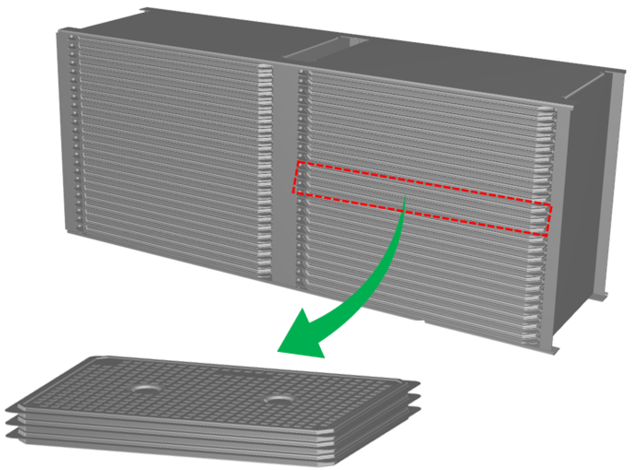
Figure 1.
Graphical overview of the application of the reduced-dimensional model to simulate the flow between the stacked heat exchanger plates.
Figure 1.
Graphical overview of the application of the reduced-dimensional model to simulate the flow between the stacked heat exchanger plates.
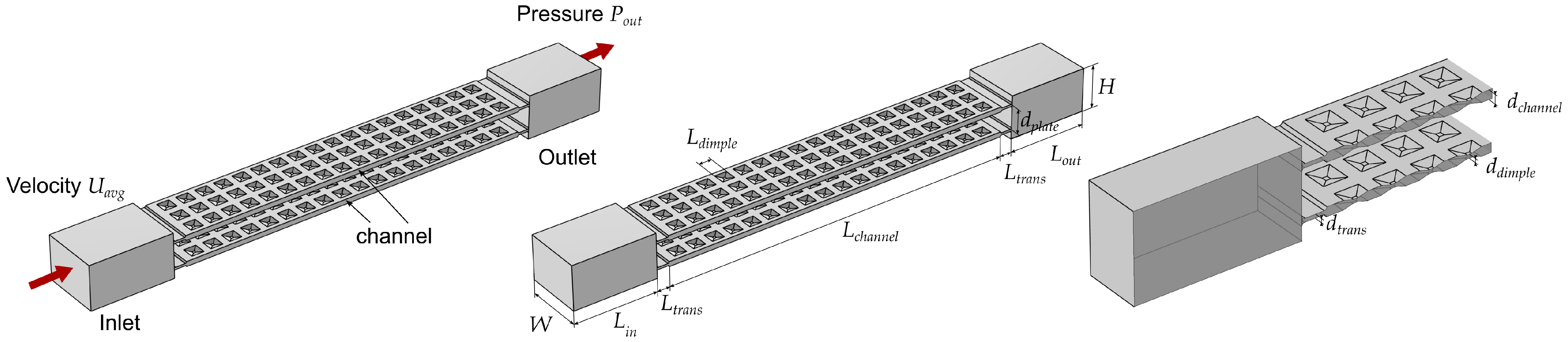
Figure 2.
Adaptation of full two-channel model from TES module consisting of stacks of plates.
Figure 2.
Adaptation of full two-channel model from TES module consisting of stacks of plates.
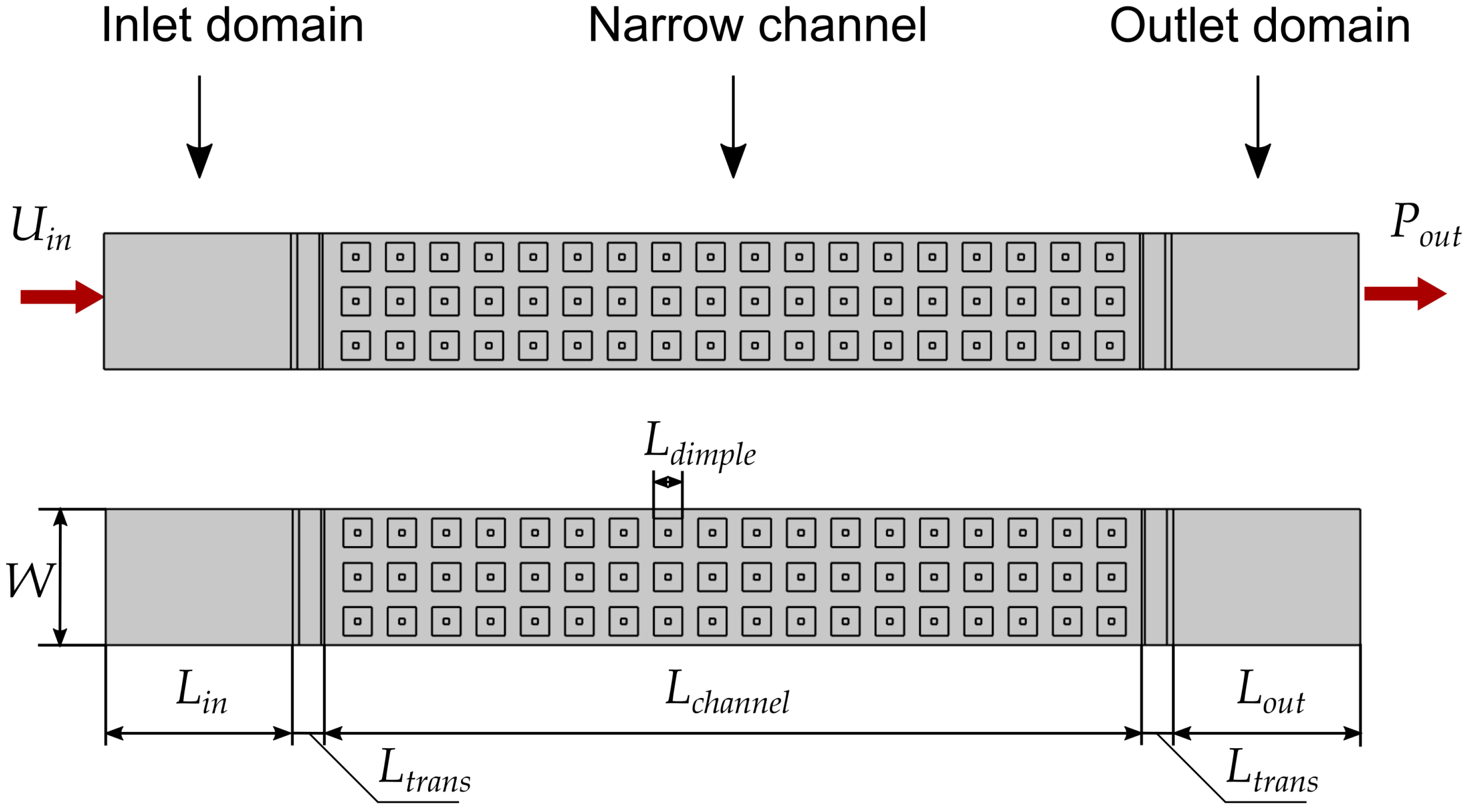
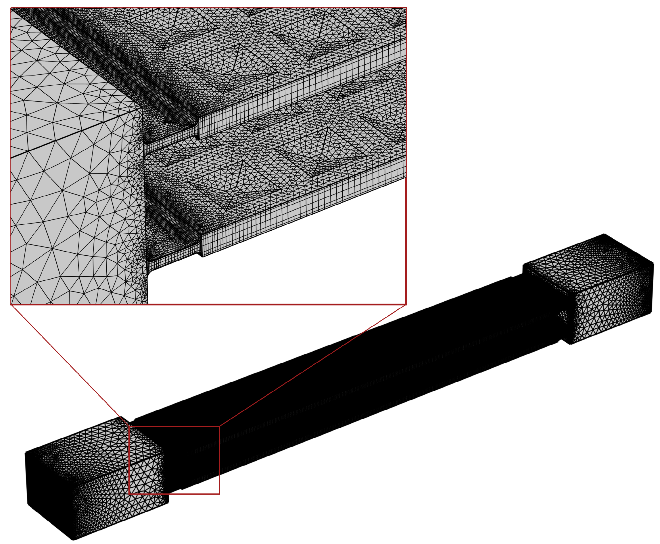
Figure 3.
Boundary conditions and dimensions for a three-dimensional sliced two-channel model. Plates are not modeled.
Figure 3.
Boundary conditions and dimensions for a three-dimensional sliced two-channel model. Plates are not modeled.
Figure 4.
Boundary conditions and dimensions for the sliced two-channel model for the reduced-dimensional model.
Figure 4.
Boundary conditions and dimensions for the sliced two-channel model for the reduced-dimensional model.
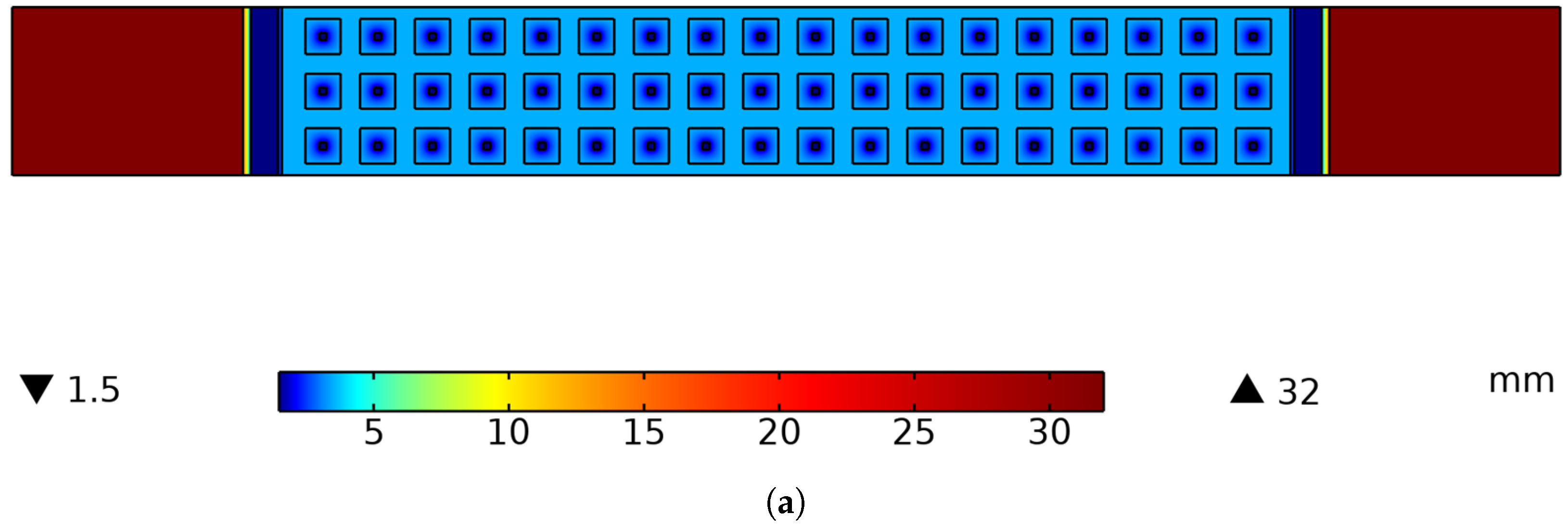
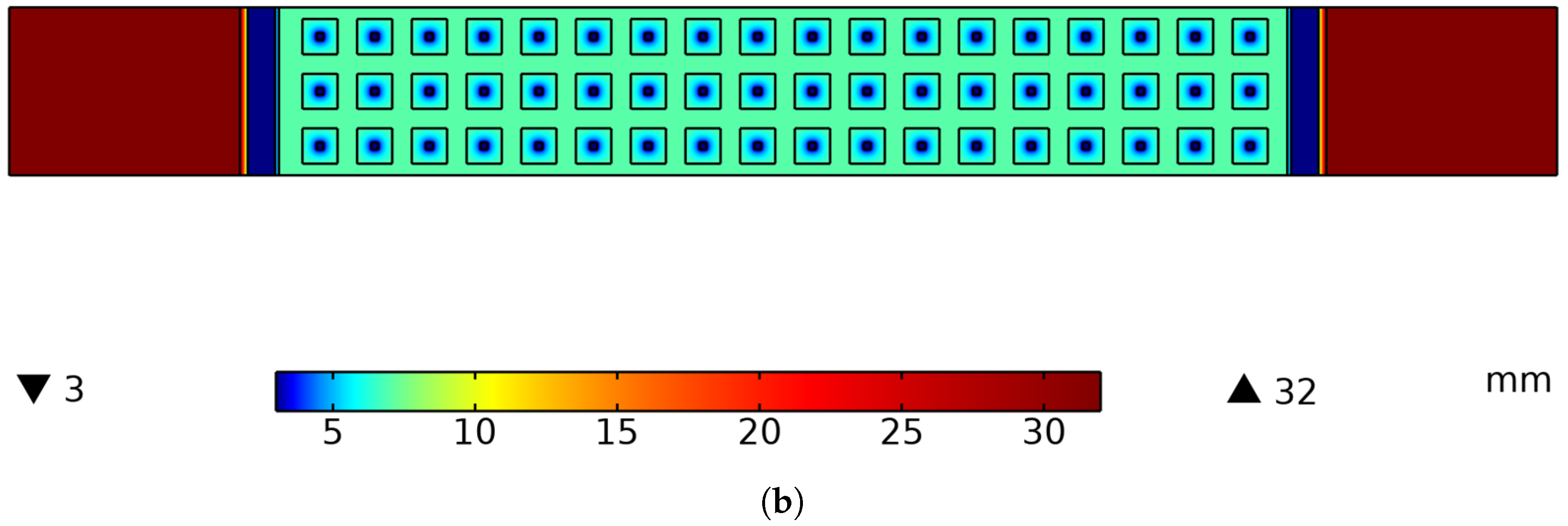
Figure 5.
Height distribution of sliced two-channel model for reduced-dimensional model. (a) Height for momentum equations, ; (b) height for mass conservation, .
Figure 5.
Height distribution of sliced two-channel model for reduced-dimensional model. (a) Height for momentum equations, ; (b) height for mass conservation, .
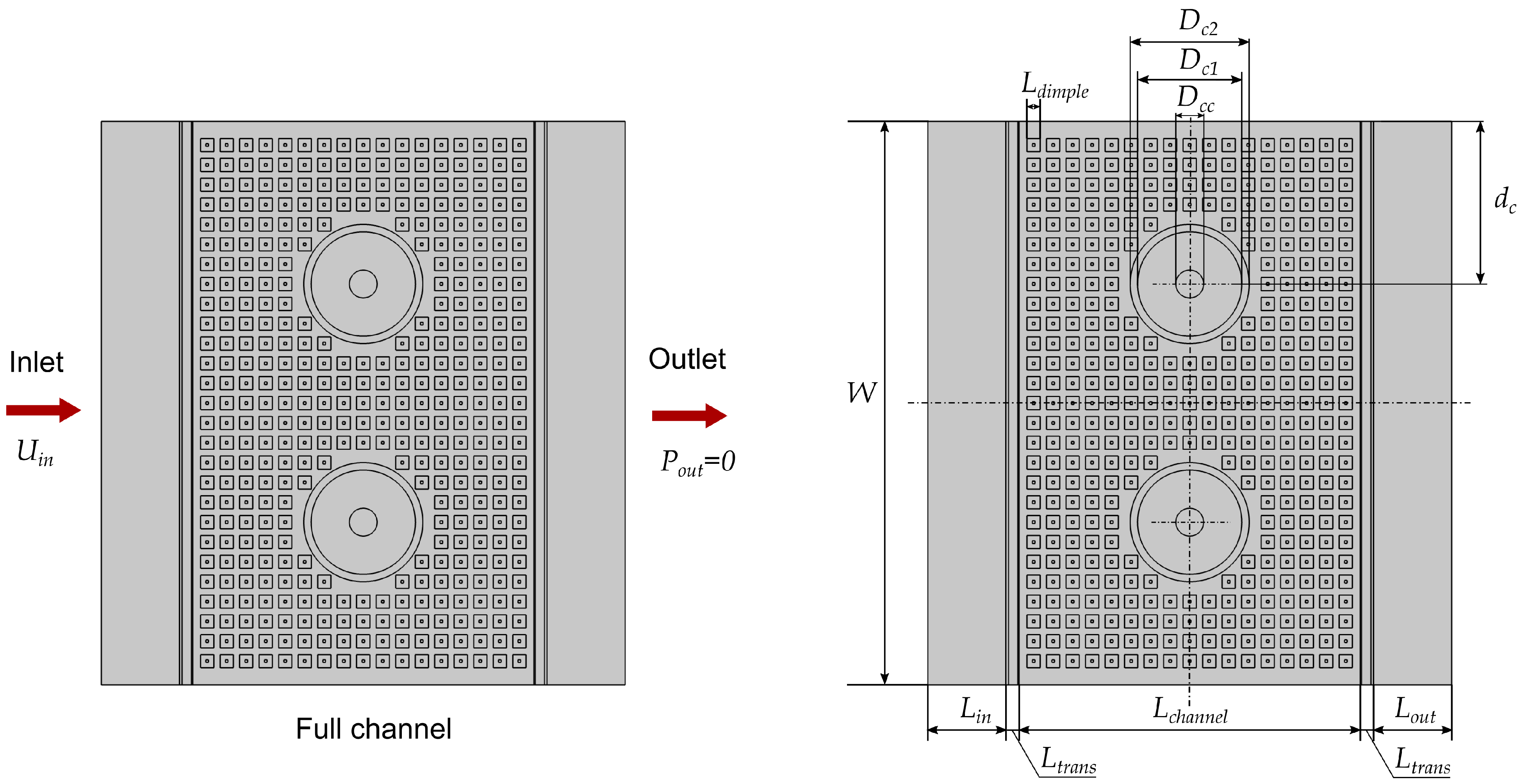
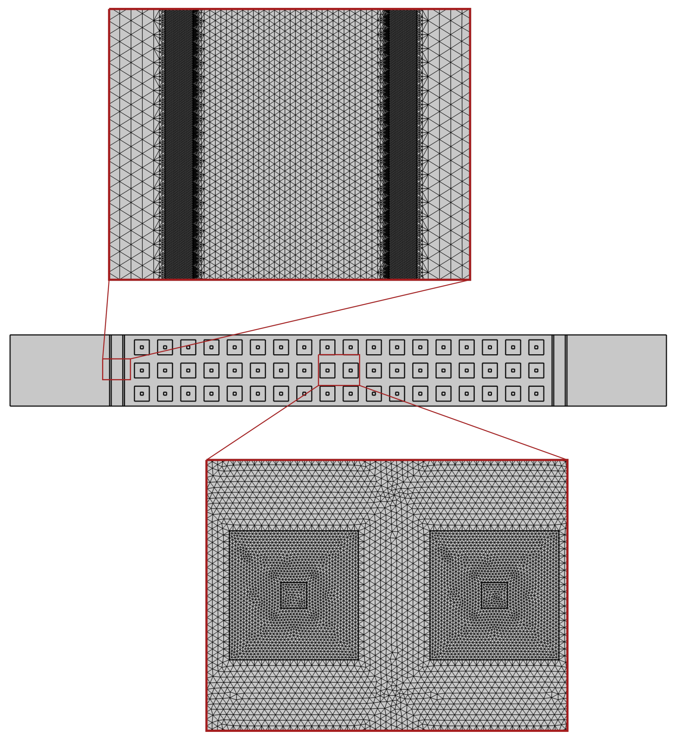
Figure 6.
Boundary conditions and dimensions for the full two-channel model for reduced-dimensional model.
Figure 6.
Boundary conditions and dimensions for the full two-channel model for reduced-dimensional model.
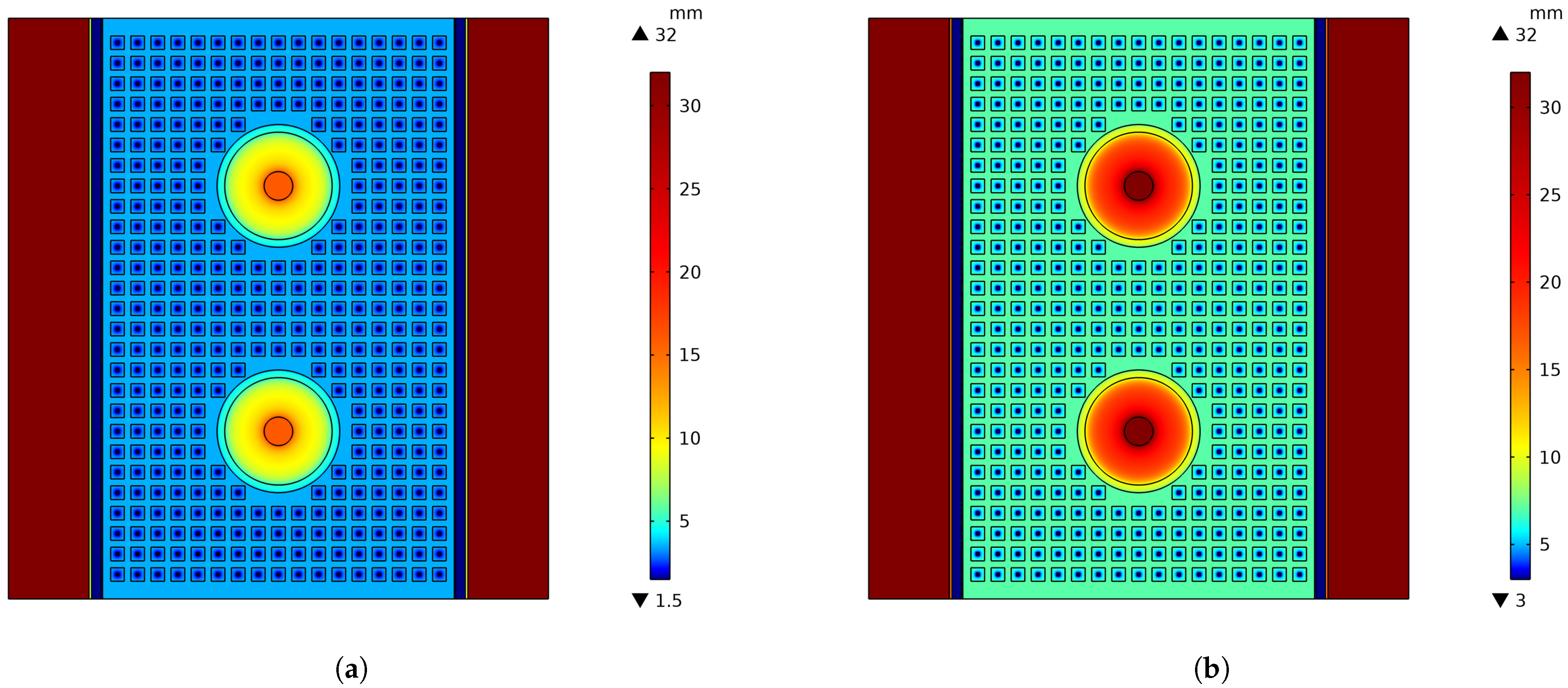
Figure 7.
Height distributions of full two-channel model for reduce-dimensional model. (a) Heights for momentum equation, ; (b) heights for mass equation, .
Figure 7.
Height distributions of full two-channel model for reduce-dimensional model. (a) Heights for momentum equation, ; (b) heights for mass equation, .
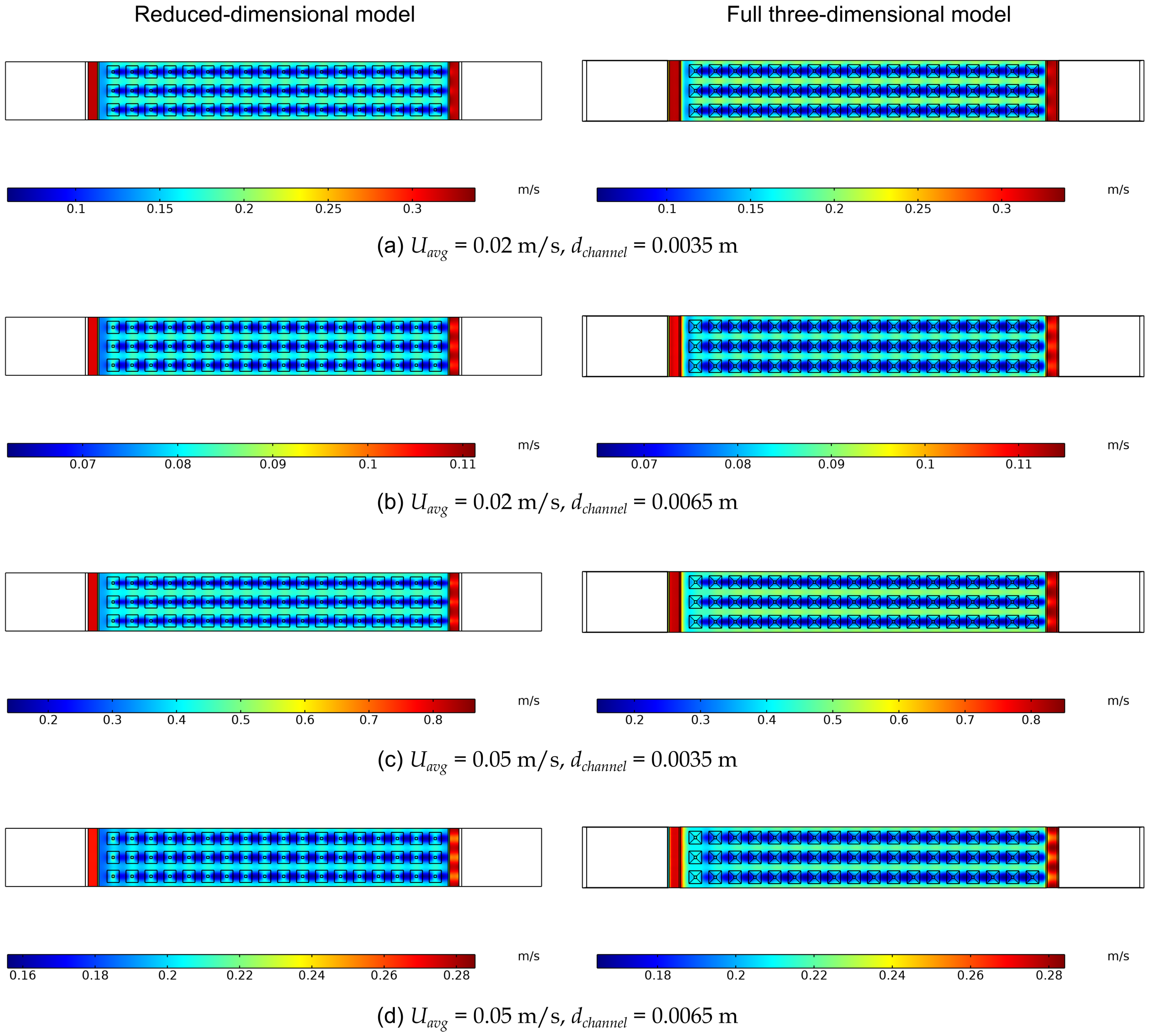
Figure 8.
Comparison of velocity distributions obtained from full three-dimensional models and reduced-dimensional models for different inlet velocities and different channel thicknesses.
Figure 8.
Comparison of velocity distributions obtained from full three-dimensional models and reduced-dimensional models for different inlet velocities and different channel thicknesses.
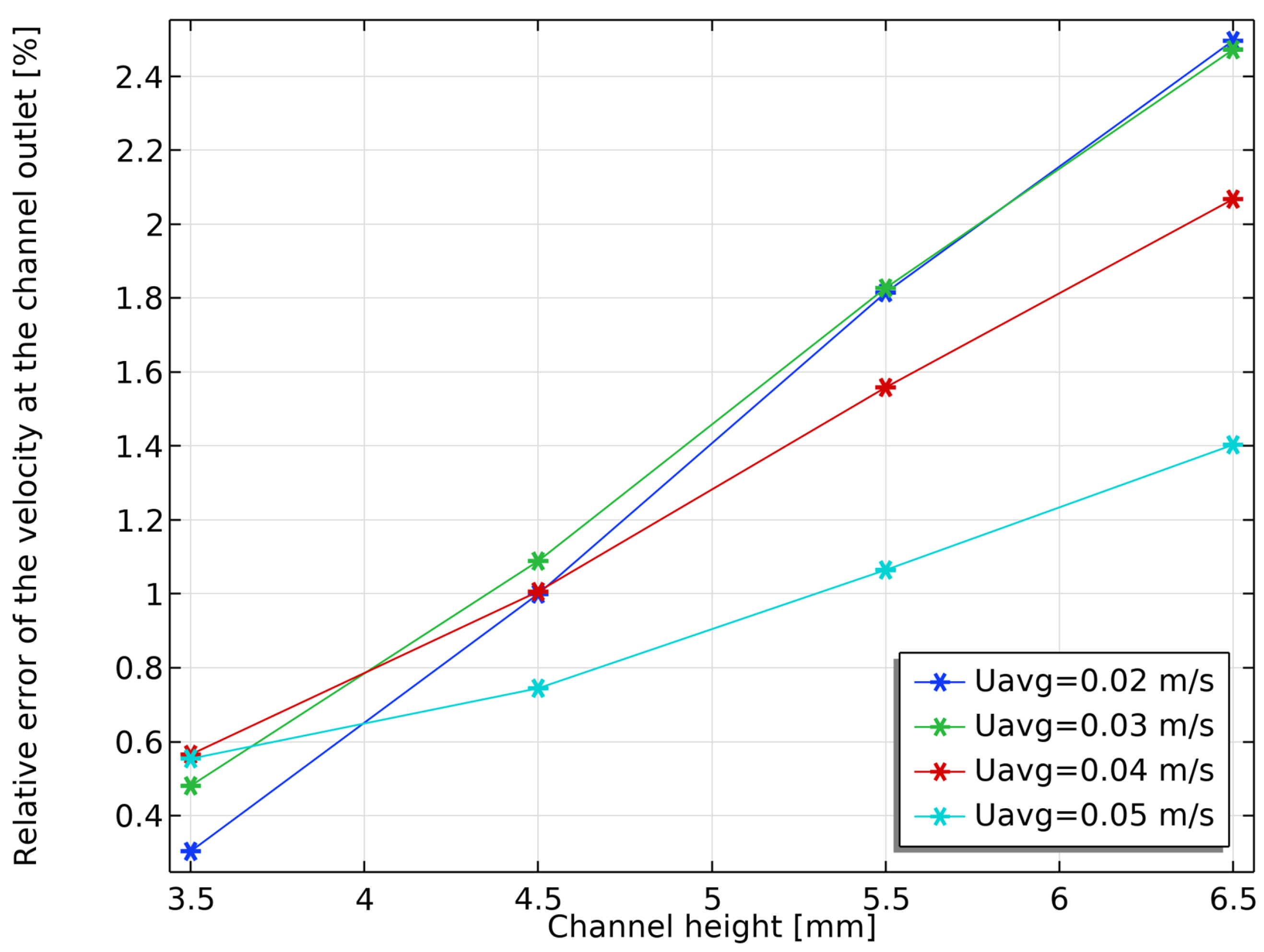
Figure 9.
Relative error of the velocity at channel outlet between reduced-dimensional model and full three-dimensional model for different inlet velocities and different channel heights.
Figure 9.
Relative error of the velocity at channel outlet between reduced-dimensional model and full three-dimensional model for different inlet velocities and different channel heights.
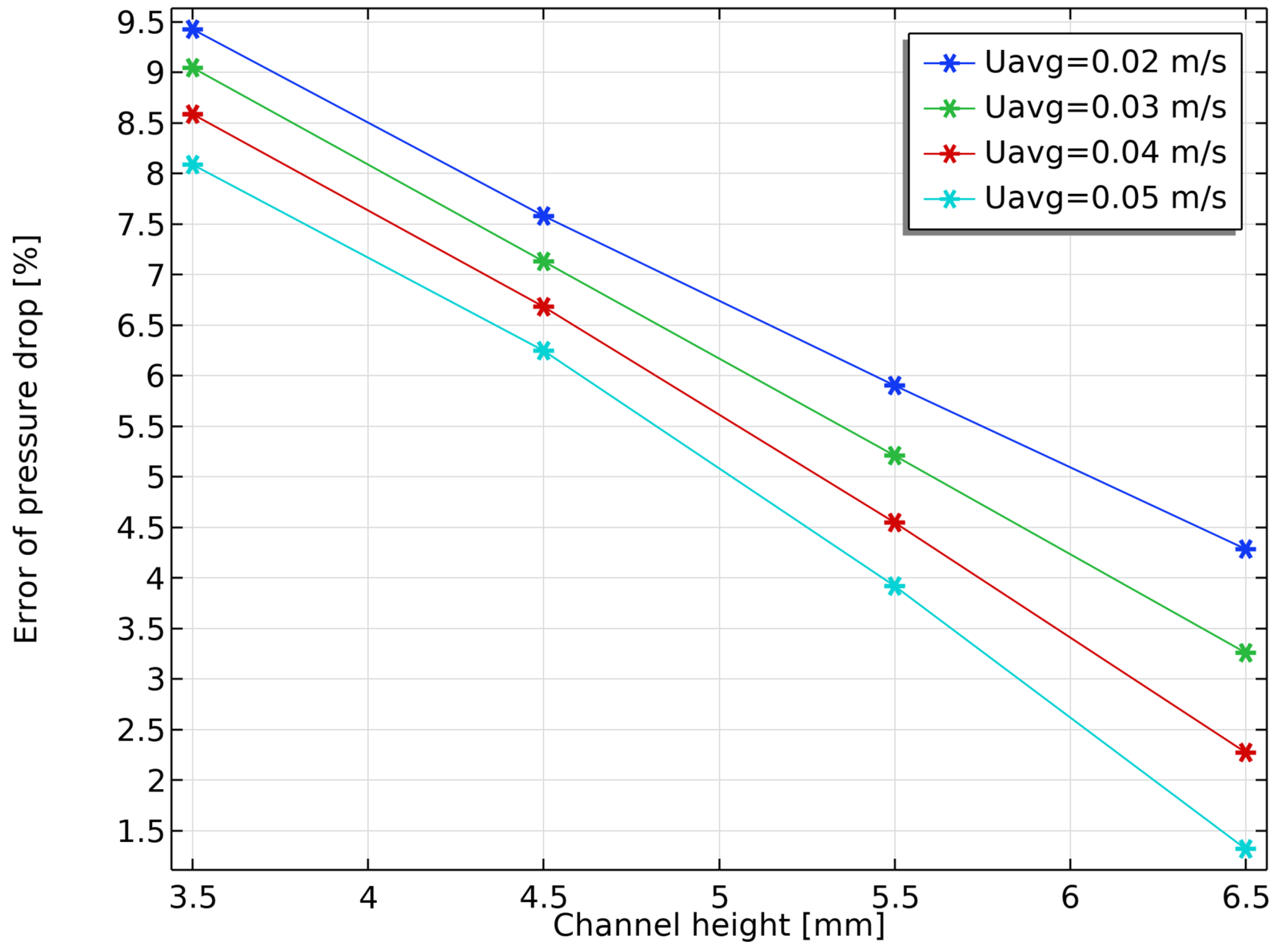
Figure 10.
Pressure drop error between reduced-dimensional model and full three-dimensional model for different inlet velocities and different channel heights.
Figure 10.
Pressure drop error between reduced-dimensional model and full three-dimensional model for different inlet velocities and different channel heights.
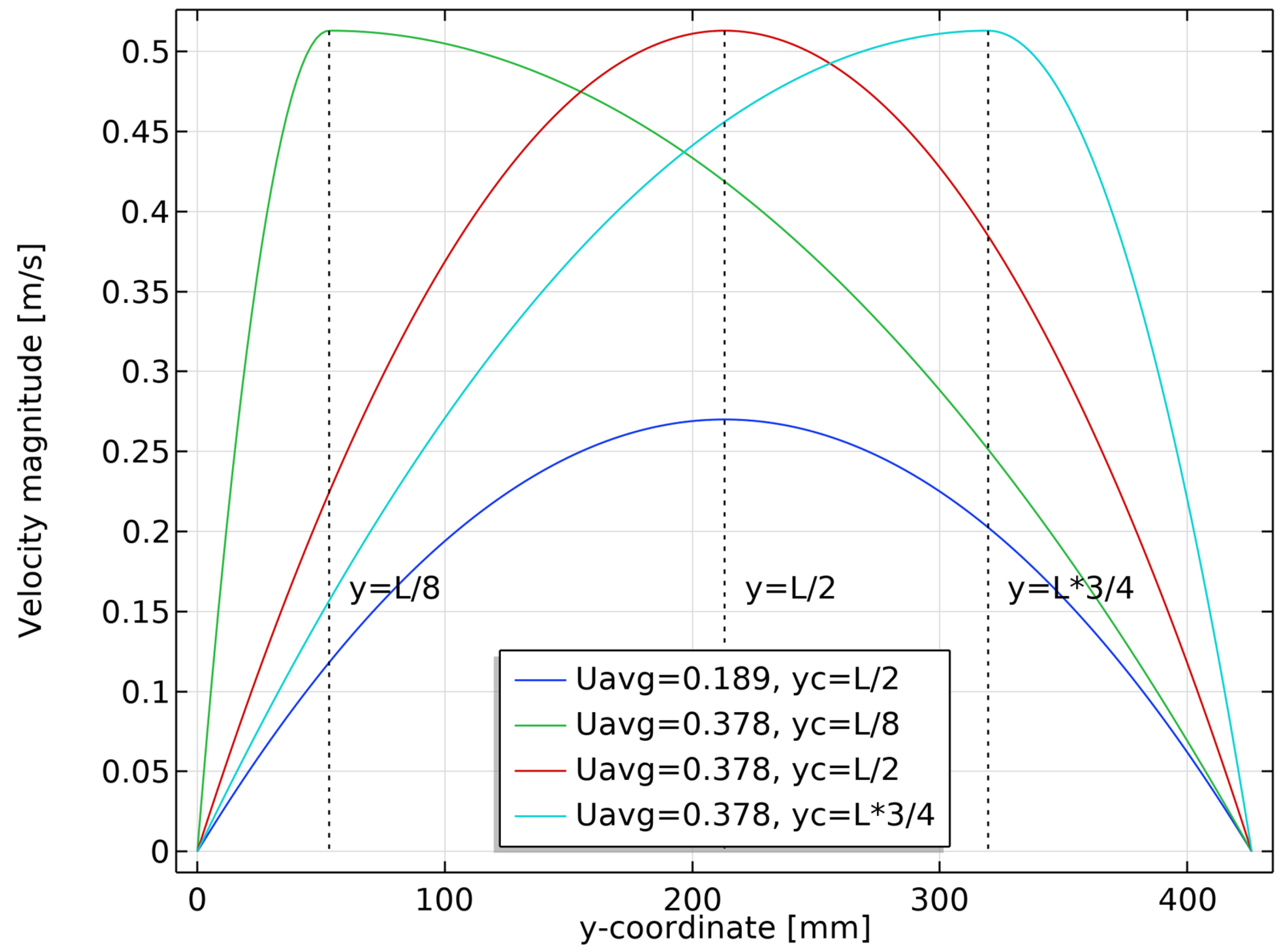
Figure 11.
Profiles of the inlet velocity for different parameters, where
controls the magnitude of the profile and
(see Equation (
6)) controls the asymmetry of the profile.
Figure 11.
Profiles of the inlet velocity for different parameters, where
controls the magnitude of the profile and
(see Equation (
6)) controls the asymmetry of the profile.
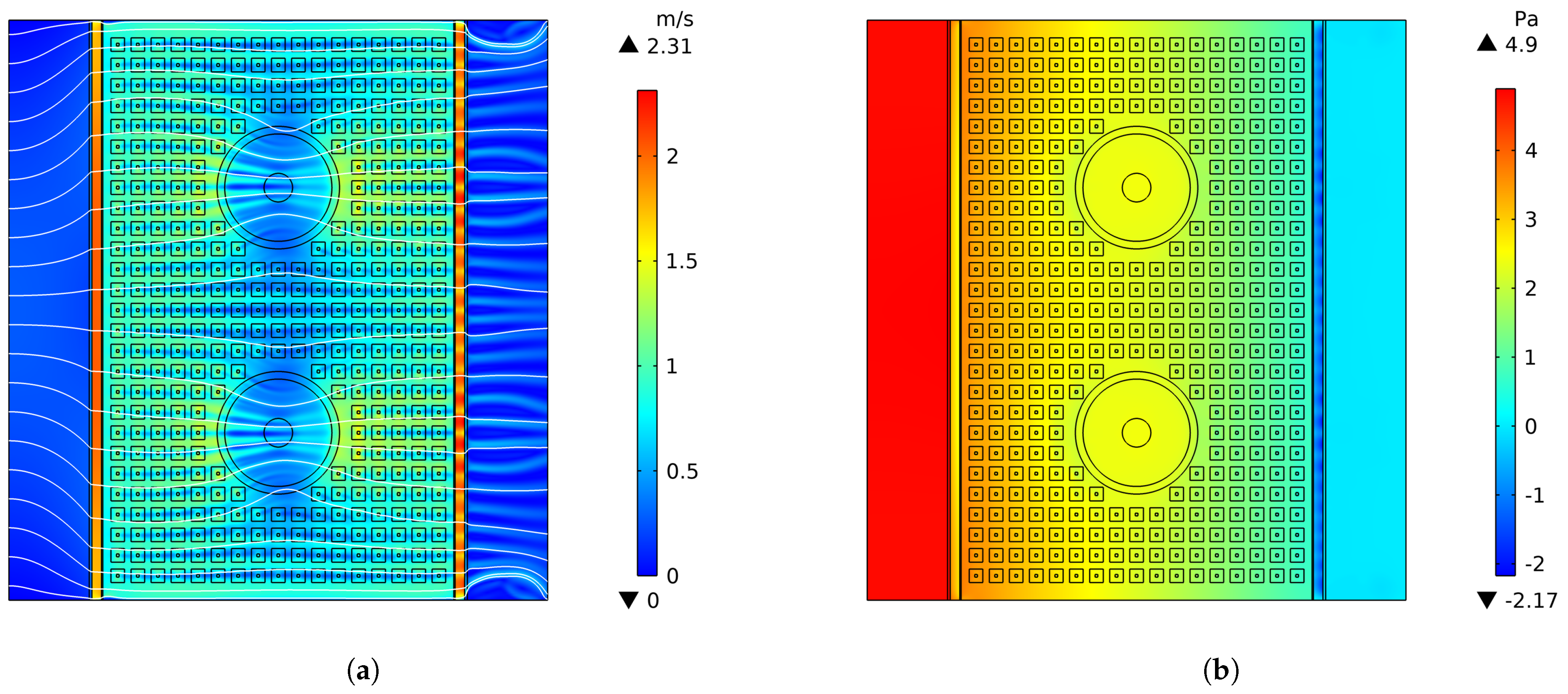
Figure 12.
Velocity and pressure distributions of the full two-channel model obtained from the reduced-dimensional model when m/s and . (a) Velocity distribution of full channel; (b) pressure distribution of full channel.
Figure 12.
Velocity and pressure distributions of the full two-channel model obtained from the reduced-dimensional model when m/s and . (a) Velocity distribution of full channel; (b) pressure distribution of full channel.
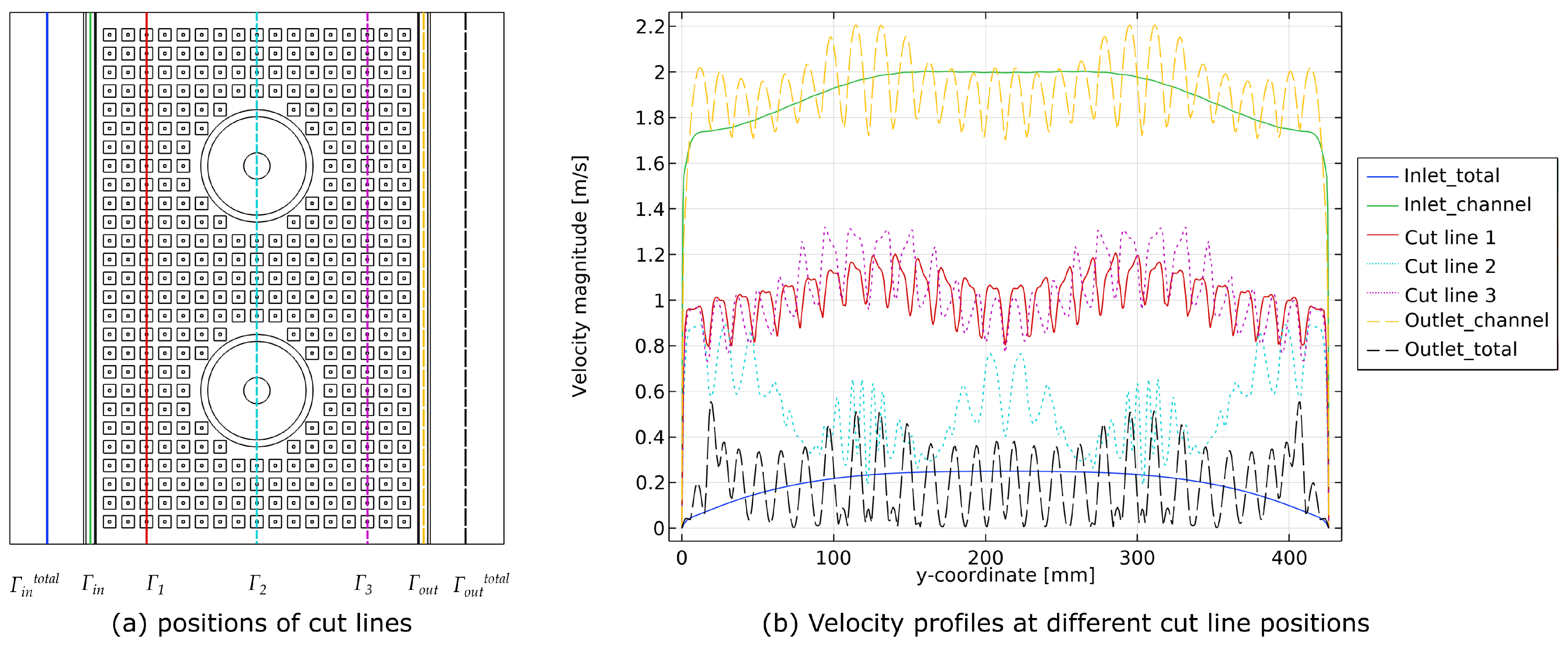
Figure 13.
Velocity profiles at different cut line positions when and m/s.
Figure 13.
Velocity profiles at different cut line positions when and m/s.
Figure 14.
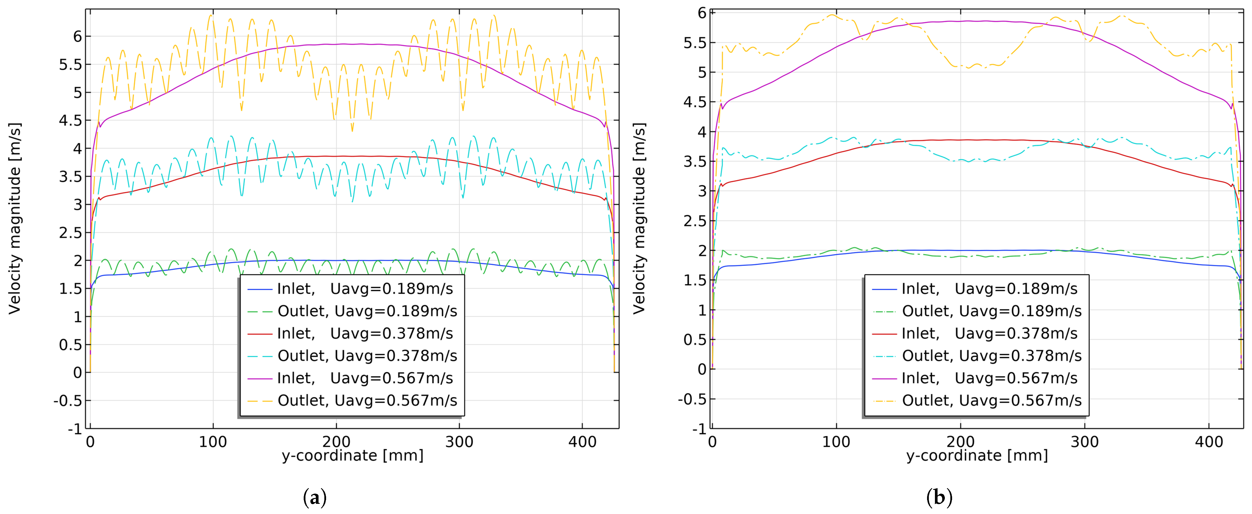
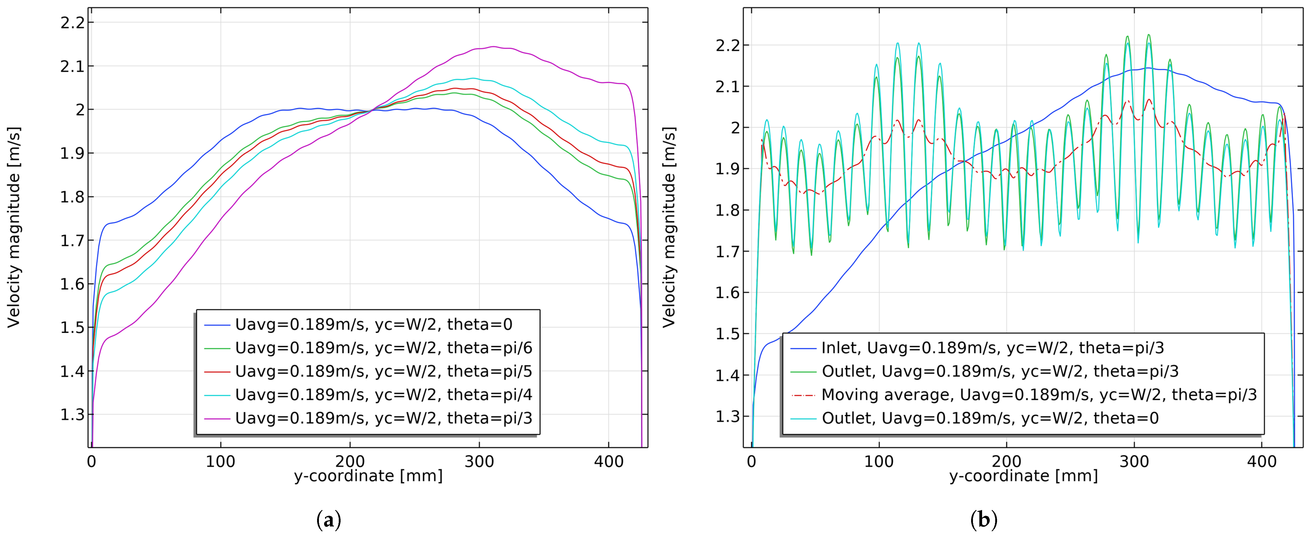
Comparison of velocity profiles over the cut lines at the channel inlet and channel outlet for different velocity magnitudes at . For (a), the solid line indicates the inlet velocity and the dashed line indicates the outlet velocity. For (b), the solid line indicates the inlet velocity and the dotted line indicates moving average velocity. (a) Velocity profiles of the channel inlet and channel outlet; (b) channel inlet velocity distribution and the moving average of the channel outlet velocity distributions.
Figure 14.
Comparison of velocity profiles over the cut lines at the channel inlet and channel outlet for different velocity magnitudes at . For (a), the solid line indicates the inlet velocity and the dashed line indicates the outlet velocity. For (b), the solid line indicates the inlet velocity and the dotted line indicates moving average velocity. (a) Velocity profiles of the channel inlet and channel outlet; (b) channel inlet velocity distribution and the moving average of the channel outlet velocity distributions.
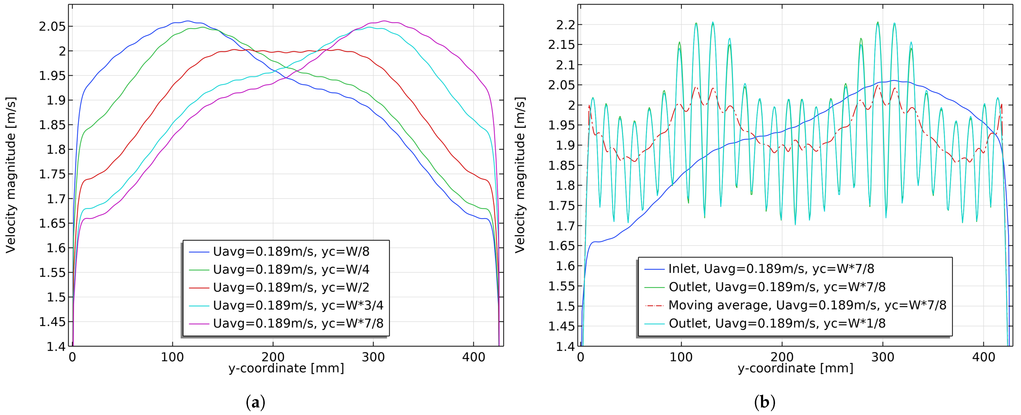
Figure 15.
Velocity profiles of the channel inlet and channel outlet for different when m/s. (a) Velocity profiles at the channel inlet for different ; (b) channel inlet and outlet velocity profiles when .
Figure 15.
Velocity profiles of the channel inlet and channel outlet for different when m/s. (a) Velocity profiles at the channel inlet for different ; (b) channel inlet and outlet velocity profiles when .
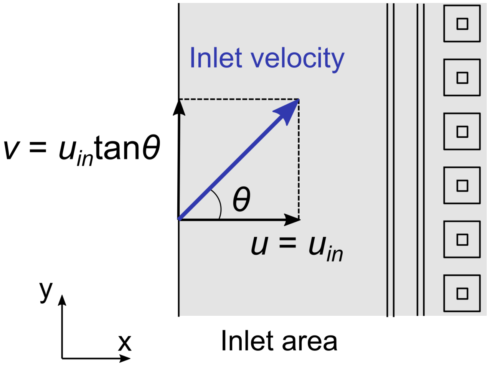
Figure 16.
Schematic diagram of the angle of inlet velocity and the velocity component.
Figure 16.
Schematic diagram of the angle of inlet velocity and the velocity component.
Figure 17.
Velocity profiles of channel inlet and channel outlet for different velocity angles when m/s and . (a) Velocity profiles at channel inlet for different velocity angles ; (b) channel inlet and outlet velocity profiles when .
Figure 17.
Velocity profiles of channel inlet and channel outlet for different velocity angles when m/s and . (a) Velocity profiles at channel inlet for different velocity angles ; (b) channel inlet and outlet velocity profiles when .
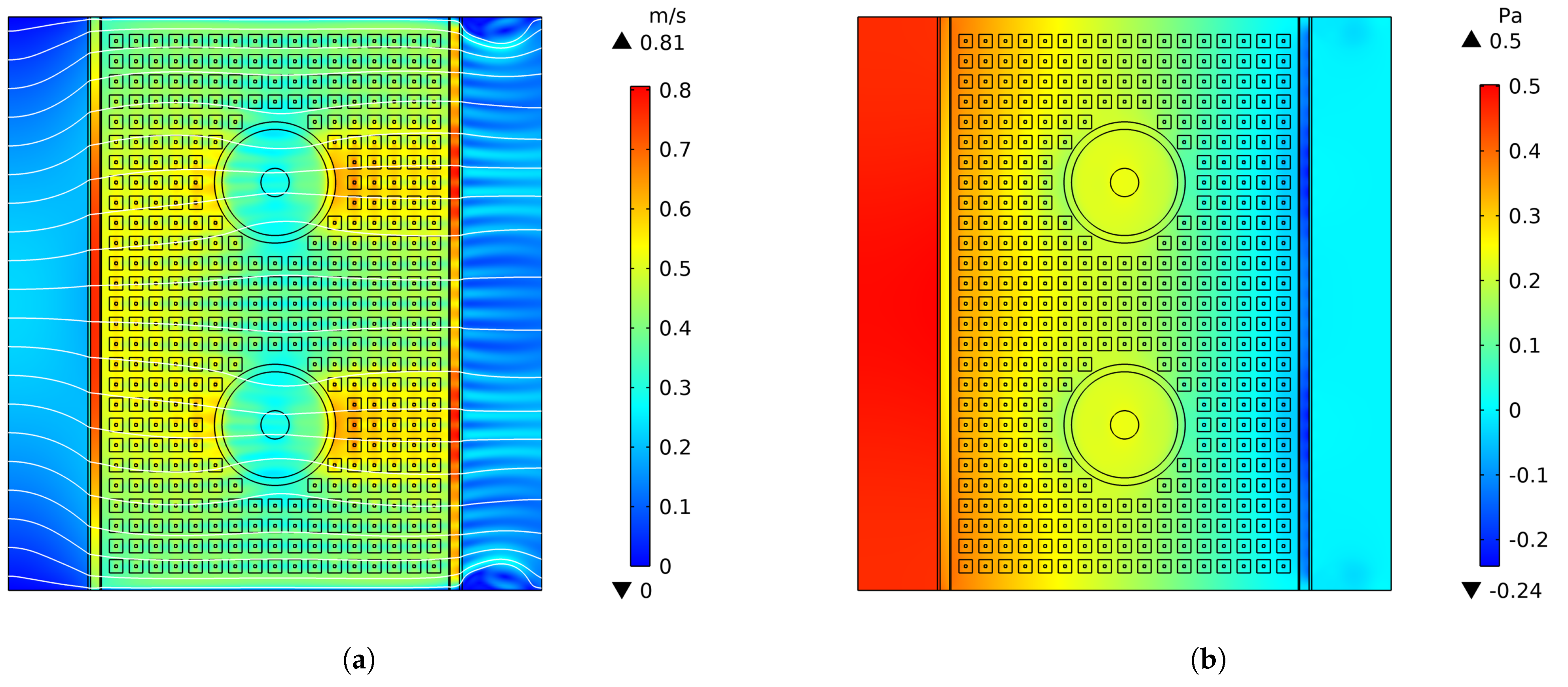
Figure 18.
Velocity and pressure distributions of the full channel when m/s, , , and the channel spacing height is 6.5 mm. (a) Velocity distribution of full channel; (b) pressure distribution of full channel.
Figure 18.
Velocity and pressure distributions of the full channel when m/s, , , and the channel spacing height is 6.5 mm. (a) Velocity distribution of full channel; (b) pressure distribution of full channel.
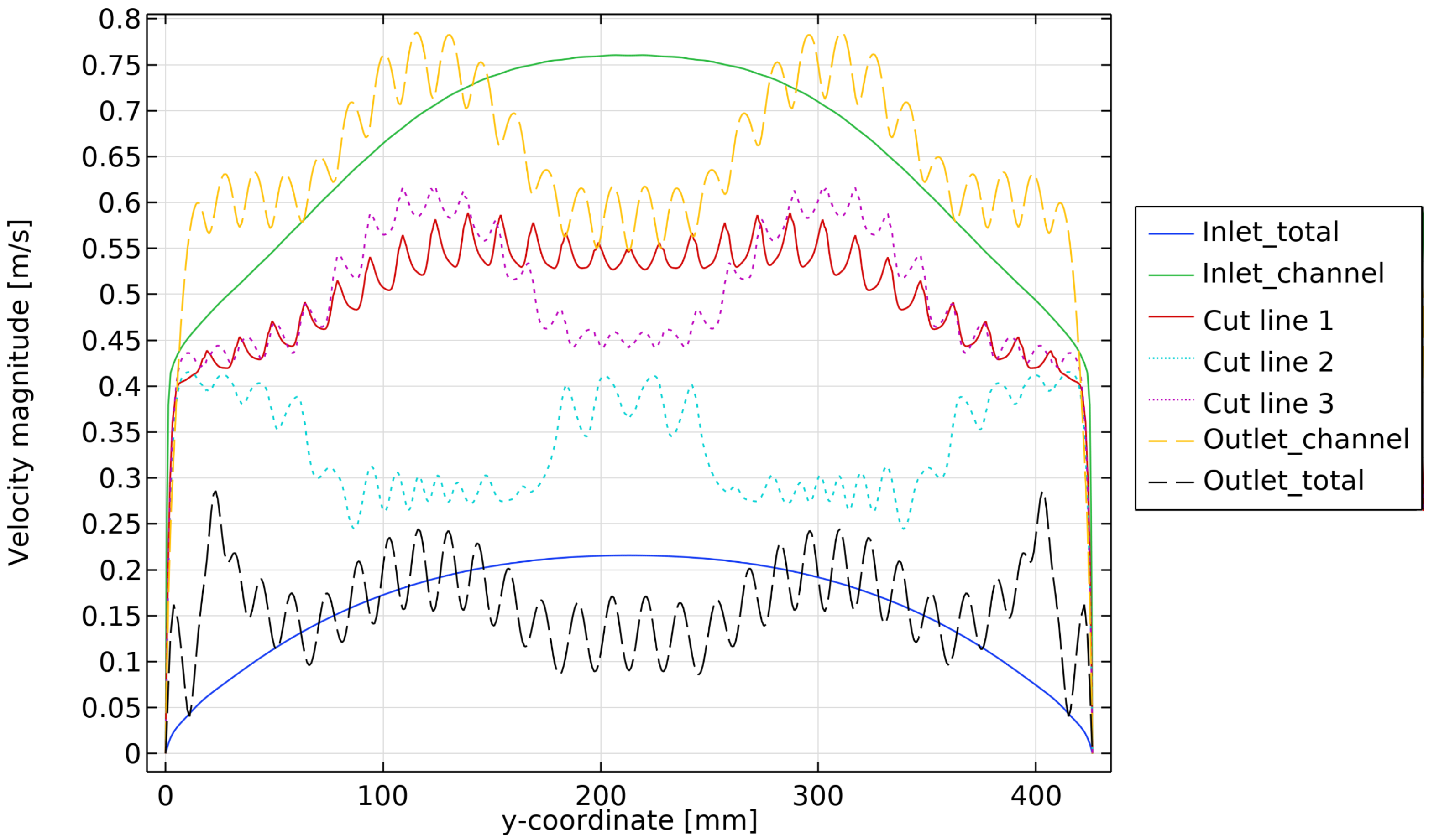
Figure 19.
Velocity profiles at different cut line positions when , , m/s, and the channel spacing height is 6.5 mm.
Figure 19.
Velocity profiles at different cut line positions when , , m/s, and the channel spacing height is 6.5 mm.
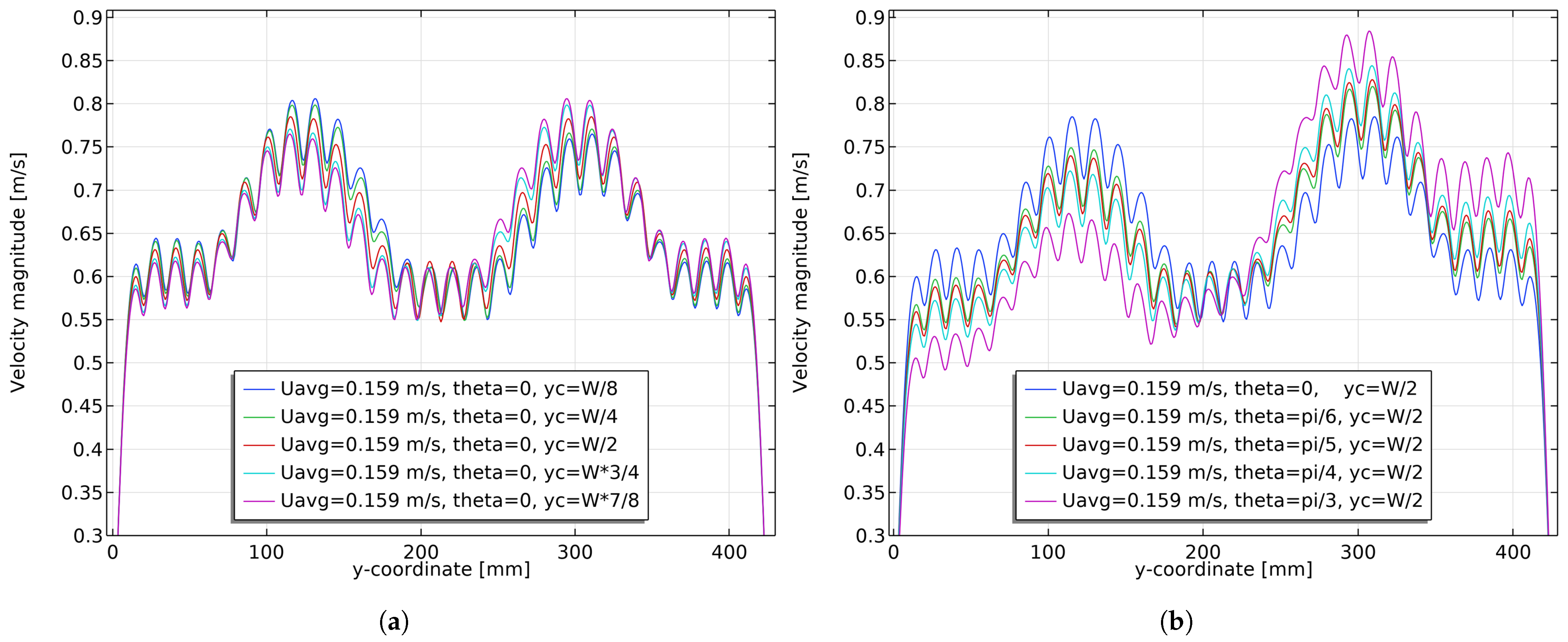
Figure 20.
Velocity profiles of the channel outlet for different when and different when . The channel spacing is 6.5 mm and the average inlet velocity is m/s. (a) Different ; (b) different .
Figure 20.
Velocity profiles of the channel outlet for different when and different when . The channel spacing is 6.5 mm and the average inlet velocity is m/s. (a) Different ; (b) different .
Table 1.
Dimensions of the sliced two-channel model (see
Figure 3) and the physical parameters of the incoming air at 27
C [
2].
Table 1.
Dimensions of the sliced two-channel model (see
Figure 3) and the physical parameters of the incoming air at 27
C [
2].
| Parameters | Symbols | Values | Units |
|---|
| Width | W | 43 | mm |
| Height | H | 32 | mm |
| Length of inlet | | 60 | mm |
| Length of outlet | | 60 | mm |
| Length of channels | | 258 | mm |
| Length of transitions | | 10 | mm |
| Length of dimples | | 9 | mm |
| Thickness of channels | | 3.5 | mm |
| Thickness of dimples | | 1.5 | mm |
| Thickness of transitions | | 1.5 | mm |
| Thickness of plates | | 15 | mm |
| Density of fluid | | 1.177 | |
| Viscosity of fluid | | | ) |
| Average inlet velocity | | 0.05 | m/s |
Table 2.
Dimensions of the full two-channel model and the physical parameters of air at 27
C [
2].
Table 2.
Dimensions of the full two-channel model and the physical parameters of air at 27
C [
2].
| Parameters | Symbols | Values | Units |
|---|
| Width | W | 426 | mm |
| Height | H | 32 | mm |
| Length of inlet | | 60 | mm |
| Length of outlet | | 60 | mm |
| Length of channels | | 258 | mm |
| Length of transitions | | 10 | mm |
| Length of dimples | | 9 | mm |
| Thickness of channels | | 3.5 | mm |
| Thickness of dimples | | 1.5 | mm |
| Thickness of transitions | | 1.5 | mm |
| Thickness of plates | | 15 | mm |
| Diameter of small circle | | 21 | mm |
| Diameter of circle 1 | | 78.8 | mm |
| Diameter of circle 2 | | 90 | mm |
| Distance between circle center and edge | | 123 | mm |
| Density of fluid | | 1.177 | |
| Viscosity of fluid | | | |
| Average inlet velocity | | 0.189 | m/s |
Table 3.
Comparison of pressure drop for different models with different inlet velocities and different channel heights.
Table 3.
Comparison of pressure drop for different models with different inlet velocities and different channel heights.
| [m/s] | [mm] | Pressure Drop [Pa] | Relative Error of Velocity [%] |
|---|
| 2D | 3D | Error [%] |
|---|
| 0.02 | 3.5 | 0.56 | 0.62 | 9.43 | 0.30 |
| 0.02 | 4.5 | 0.25 | 0.27 | 7.58 | 1.00 |
| 0.02 | 5.5 | 0.13 | 0.14 | 5.90 | 1.81 |
| 0.02 | 6.5 | 0.08 | 0.08 | 4.29 | 2.50 |
| 0.03 | 3.5 | 0.85 | 0.93 | 9.05 | 0.48 |
| 0.03 | 4.5 | 0.37 | 0.40 | 7.13 | 1.09 |
| 0.03 | 5.5 | 0.19 | 0.20 | 5.21 | 1.83 |
| 0.03 | 6.5 | 0.11 | 0.12 | 3.26 | 2.47 |
| 0.04 | 3.5 | 1.13 | 1.24 | 8.59 | 0.57 |
| 0.04 | 4.5 | 0.49 | 0.53 | 6.68 | 1.01 |
| 0.04 | 5.5 | 0.26 | 0.27 | 4.55 | 1.56 |
| 0.04 | 6.5 | 0.15 | 0.16 | 2.27 | 2.07 |
| 0.05 | 3.5 | 1.42 | 1.54 | 8.09 | 0.55 |
| 0.05 | 4.5 | 0.62 | 0.66 | 6.25 | 0.74 |
| 0.05 | 5.5 | 0.32 | 0.34 | 3.92 | 1.06 |
| 0.05 | 6.5 | 0.19 | 0.19 | 1.32 | 1.40 |
Table 4.
Average velocity and standard deviation of the inlet and outlet of the channel and the moving average of the outlet velocity for different velocity magnitudes.
Table 4.
Average velocity and standard deviation of the inlet and outlet of the channel and the moving average of the outlet velocity for different velocity magnitudes.
| [m/s] | Average Velocity [m/s] | Standard Deviation [-] |
|---|
| Inlet | Outlet | Mov. avg. | Inlet | Outlet | Mov. avg. |
|---|
| 0.189 | 1.9345 | 1.9367 | 1.9364 | 0.0998 | 0.1259 | 0.0528 |
| 0.378 | 3.6759 | 3.6951 | 3.6953 | 0.2590 | 0.2658 | 0.1295 |
| 0.567 | 5.5148 | 5.5600 | 5.5612 | 0.4778 | 0.4466 | 0.2709 |
Table 5.
Average velocity and standard deviation of the inlet and outlet of the channel and the moving average of the outlet velocity for different when m/s.
Table 5.
Average velocity and standard deviation of the inlet and outlet of the channel and the moving average of the outlet velocity for different when m/s.
| [mm] | Average Velocity [m/s] | Standard Deviation [-] |
|---|
| Inlet | Outlet | Mov. avg. | Inlet | Outlet | Mov. avg. |
|---|
| W/8 | 1.9392 | 1.9368 | 1.9365 | 0.1254 | 0.1252 | 0.0529 |
| W/4 | 1.9366 | 1.9367 | 1.9364 | 0.1115 | 0.1256 | 0.0529 |
| W/2 | 1.9345 | 1.9367 | 1.9364 | 0.0998 | 0.1259 | 0.0528 |
| 3W/4 | 1.9366 | 1.9366 | 1.9364 | 0.1113 | 0.1257 | 0.0530 |
| 7W/8 | 1.9392 | 1.9367 | 1.9364 | 0.1251 | 0.1253 | 0.0530 |
Table 6.
Average velocity and standard deviation of the inlet and outlet of the channel and the moving average of the outlet velocity for different when m/s, .
Table 6.
Average velocity and standard deviation of the inlet and outlet of the channel and the moving average of the outlet velocity for different when m/s, .
| [rad] | Average Velocity [m/s] | Standard Deviation [-] |
|---|
| Inlet | Outlet | Mov. avg. | Inlet | Outlet | Mov. avg. |
|---|
| 0 | 1.9345 | 1.9367 | 1.9364 | 0.0998 | 0.1259 | 0.0528 |
| 1.9358 | 1.9367 | 1.9364 | 0.1181 | 0.1258 | 0.0534 |
| 1.9366 | 1.9367 | 1.9364 | 0.1277 | 0.1256 | 0.0536 |
| 1.9385 | 1.9366 | 1.9363 | 0.1485 | 0.1255 | 0.0542 |
| 1.9467 | 1.9366 | 1.9363 | 0.2149 | 0.1256 | 0.0562 |


