1. Introduction
Many cooling systems for main and auxiliary equipment, as well as safety systems related to the removal of residual heat in reactor units of land-based and floating nuclear power plants, use the method of moving heat to the atmosphere. To accomplish this, various air-cooled heat exchanger designs are used, including different geometry on the heat exchange surface or different types of air circulation (natural or forced convection). The efficiency of heat transfer in such devices depends on several factors, such as the flow rate of the medium to be cooled, its inlet temperature, and the temperature and speed of the ambient air. These parameters are usually not constant and depend both on the characteristics of the technological process and on weather conditions.
The heat exchange surfaces of modern air-cooled heat exchangers have a complex shape since simple straight-tube or smooth plate elements do not allow achieving high heat transfer coefficients; these complex shapes lead to an increase in the overall dimensions of the heat exchanger.
One option to make the heat exchanger’s design more compact is the use of close-packed with small bend radius coils (SBRC). Such designs [
1] have been applied in various industries. However, heat transfer in the complex geometry of a heat exchanger’s annular space (
Figure 1) cannot be described by simple one-dimensional cases and dependencies; for example, formulas for the heat transfer coefficient of a transverse flow around a tube bundle must consider the three-dimensional spatial structure of the heat exchange surface.
At present, there is a fairly universal and proven tool for modeling the thermal-hydraulic characteristics of a coolant in channels of complex shape: computational fluid dynamics. However, the dimension of computational grids can require billions of finite volumes to simulate full-scale heat-exchange installations with SBRC because describing the geometry of the heat exchange surface qualitatively requires grid elements of 0.1–1 mm in size are required, and the entire installation has an overall dimension of several meters. Calculations on such grids will require significant computer time and the use of powerful supercomputers.
An alternative to this approach can be the use of reduced order models (ROM-models), in which the computational domain is not modeled directly. Instead, it is described through simplified models, such as a porous medium model. However, such a model requires additional closing relations and coefficients that characterize the actual channel geometry.
2. Heat Exchanger with SBRC
At NNSTU n.a. R.E. Alekseev (Nizhny Novgorod, Russia), an experimental thermophysical facility FT-40 [
2,
3] was created to study the processes of mixing non-isothermal flows of water coolant in models of equipment for nuclear power plants. This research facility is universal and multifunctional, which causes periodic changes in both its operating modes and the design of working sections, as well as the requirements for accuracy in maintaining the specified thermophysical parameters of the working environment.
These factors necessitate periodic changes in the algorithms of the automated control system of the stand. Considering the high energy consumption for conducting non-isothermal experiments at this facility, optimization and development of control algorithms and maintaining parameters at an operating facility can be very expensive and time-consuming. One way to solve this problem is to create digital twins of the stand equipment; this would allow operating modes to be modeled and optimized in advance.
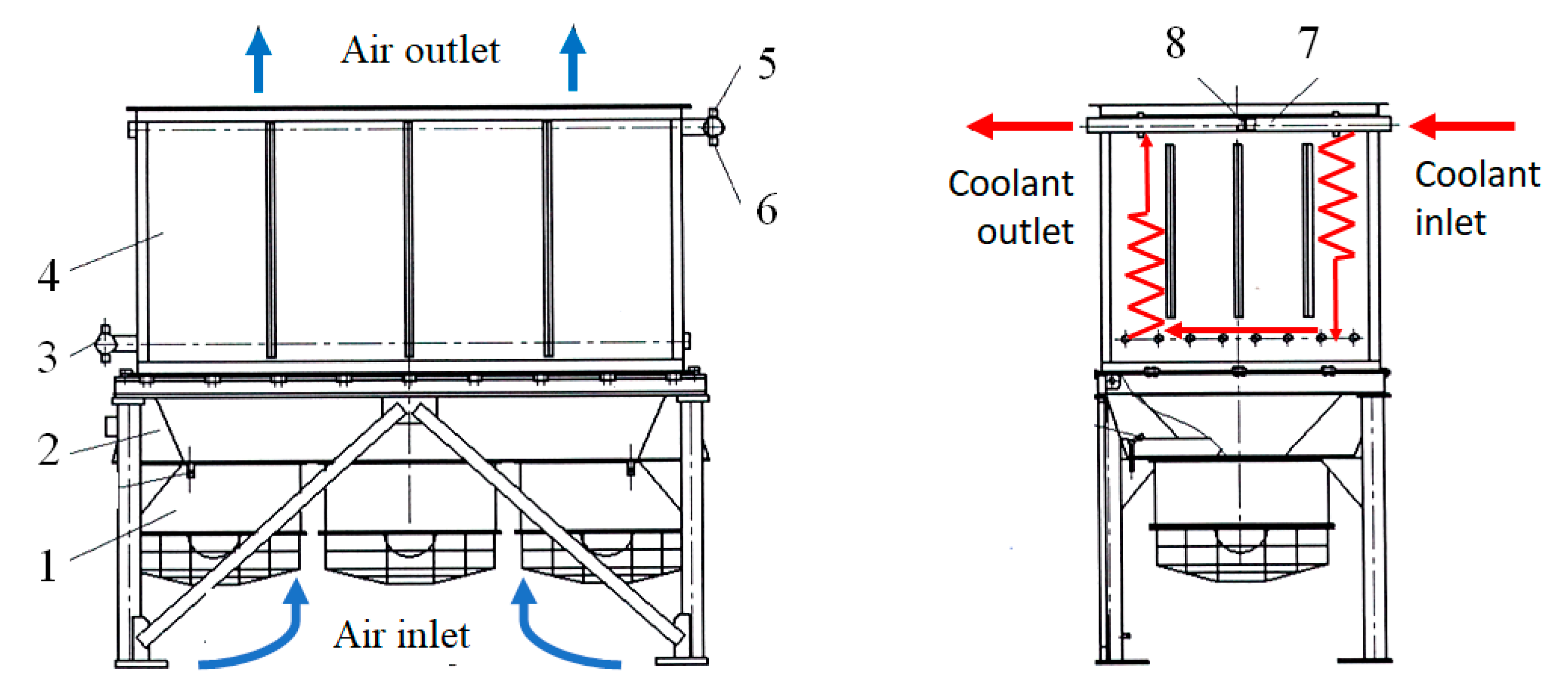
An important requirement in carrying out experimental studies is to maintain a constant temperature of the working medium flows at the inlet to the model being studied. For heated streams, this is ensured by using electric heaters with thyristor controllers, which allow the heating power to be adjusted. To cool the flows, an air-cooled heat exchanger with a forced supply of atmospheric air is used, which is the object of modeling In this work.
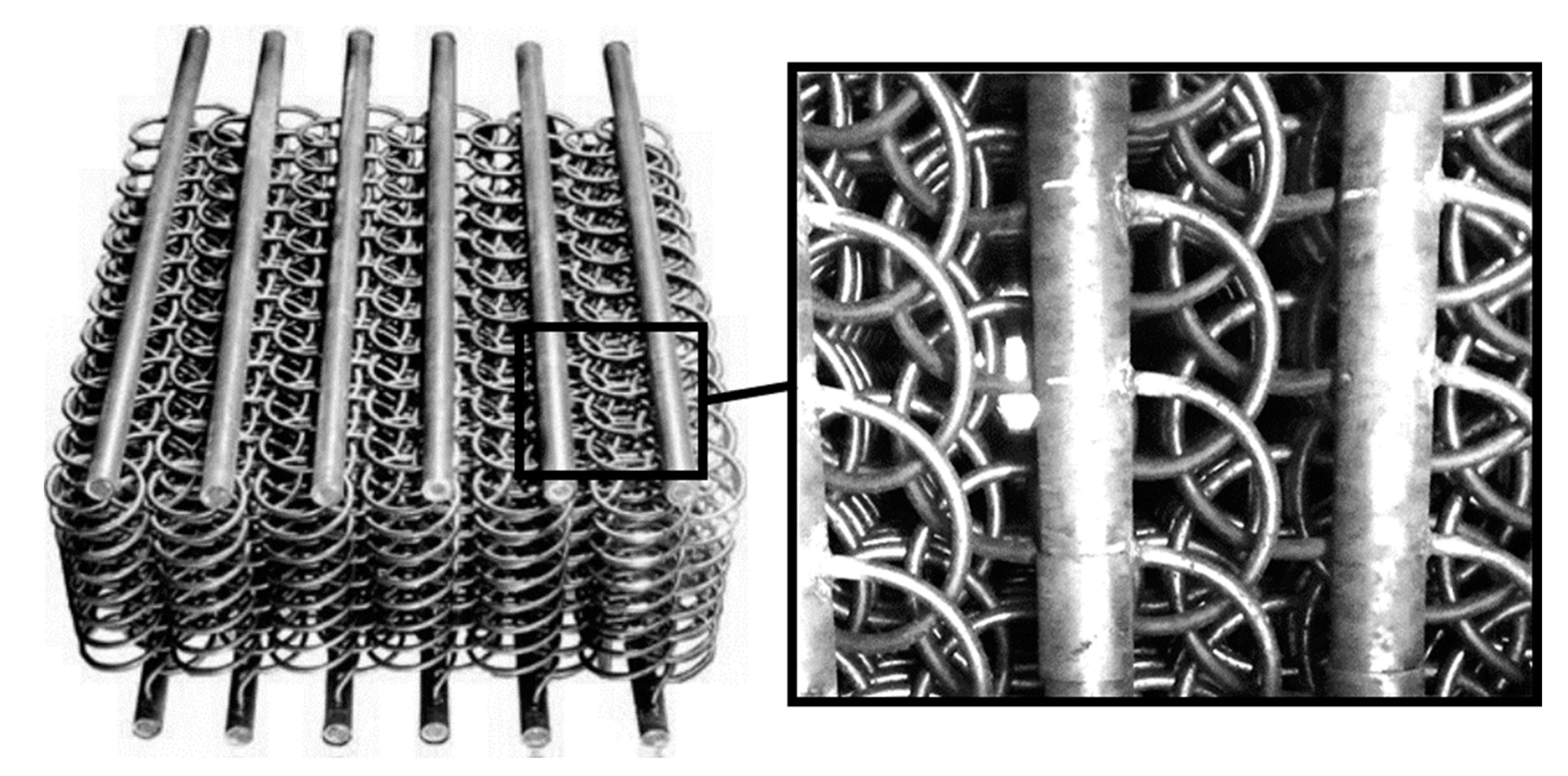
The heat exchange surface of the air-cooled heat exchanger (
Figure 2) consists of SBRC. The coils are combined into eight vertically arranged modules. The modules are connected by upper and lower collectors.
The heat exchanger has a two-way circuit for circulation of the cooled medium. The upper collector is divided by a sealed partition into two cavities. The cooled medium enters one of the cavities of the upper manifold, passes down the coils of four modules, enters the lower manifold, and through it, enters the next four modules. Then, it rises up the coils and exits through another cavity in the upper collector.
Atmospheric air is supplied by three lower fans to the heat exchange unit, passes between the coils and exits at the top. The automated control system provides an algorithm that turns on the fans when the temperature of the cooled medium at the inlet to the heat exchanger reaches a predetermined setpoint. to the fan speed can also be changed using a frequency converter. This ensures that the temperature of the cooled medium at the outlet is maintained at a variable inlet temperature.
Simulation of air flow in the entire annular space of a heat exchanger 4500 × 2000 × 1700 mm in size with reproduction of the real geometry of the coils using computational fluid dynamics programs is an extremely resource-intensive task as it requires a finite volume mesh with several billion elements and high-performance supercomputer equipment.
One of the possible simplifications of the computational model is the use of a porous medium model. Simplified numerical models are currently used by many researchers in various fields of science and technology, including nuclear installations, aircraft engine heat exchangers, medical and chemical devices, filter elements, heat exchangers for microelectronics and automotive industry, and electric heaters. Also, such models are used directly to model the flow of liquid and gaseous media in porous structures.
Paper [
4] presented the results of a numerical simulation of coolant flow through bundles of cylindrical rods with both longitudinal and transverse flow. Such rod assemblies are typical for nuclear power plant equipment. The authors of this article used the model of a non-isotropic porous medium to simulate processes, which made it possible to significantly reduce the calculation time. The authors of work [
5] applied the porous medium model to simulate the core of a nuclear reactor, supplementing it with a heat transfer model. Papers [
6,
7,
8] presented the results of using porous medium models to calculate the thermal hydraulics of nuclear power plant equipment. In each of these studies, the models were used to reduce the calculation time while maintaining a sufficient level of modeling accuracy.
In papers [
9,
10], a simplification of CPD models using a porous medium was applied to study the distribution of heat flow and evaluate the efficiency of heat transfer in aircraft equipment and intercooled recuperated aero engines. The described numerical tool is based on an advanced porosity model approach where the heat exchanger core is modeled as a porous media of predefined heat transfer and pressure loss behavior. Additionally, the derived porosity model is able to provide accurate results to a wide range of conditions.
In paper [
11], several alternative geometries of hemodialysis modules were simulated by means of a computational fluid dynamics model. This is based on a porous media treatment and accounts for both diffusive and convective (ultrafiltration) fluxes. The simulated configurations differed in geometry and flow path, including mainly longitudinal and mainly transverse flow. The use of the porous medium model was required because the characteristic dimensions of the blood flow channel in these medical devices differed by several orders of magnitude from the overall dimensions of the computational domain. Direct modeling of the geometry with the standard CFD approach would require a very large number of mesh elements.
In study [
12], the dry pressure drop in the cross-flow rotating packed bed was investigated using computational fluid dynamics. The packing was modeled by the porous media model and the rotation of the packing was simulated by the sliding mesh model.
The pneumatic conveying process of fine particles through filters was studied in paper [
13] using the CFD simulation method. The porous media model and porous structure were used to simulate the airflow state and the blocking effect of fine particles when they flowed through the filter.
In study [
14], a novel methodology is developed to model the microchannels as a porous medium where a compressible gas is used as a working fluid. The authors showed that such an approach was needed because micro heat exchangers include distributing and collecting manifolds as well as hundreds of parallel microchannels, so a complete CFD conjugate heat transfer analysis requires a large amount of computational power and the use of a porous medium model can reduce computational costs.
Papers [
15,
16,
17,
18,
19] also used a simplification of the numerical model since a porous medium was used. In these works, the thermal and hydrodynamic characteristics of the devices under study were determined, and those devices featured very small flow channel dimensions compared to the overall dimensions.
Thus, the objectives of present study were:
- −
developing a numerical model for an air-cooled heat exchanger, in which the heat exchange surface is described based on studying the air flow in a porous medium model, using a personal computer over a short period of time;
- −
developing a realistic numerical model of a fragment of the assembly of coils using the values for the heat transfer coefficients and hydraulic resistance, which are necessary for a porous medium model;
- −
modeling the operation of an air-cooled heat exchanger in various modes that are differentiated by the number of fans turned on and their rotation speed, as well as determining the value of the thermal power that the air removes.
3. Numerical Models and Methods
3.1. Porous Medium Model in CFD
To compile a numerical model of a heat exchanger with SBRC, the Ansys CFX 19.0 program was used.
The volume porosity γ at a point is the ratio of the volume
V′ available to flow in an infinitesimal control cell surrounding the point, and the physical volume
V of the cell. Hence:
It is assumed that the area available to flow
A’ through an infinitesimal planar control surface of porous medium area
A is given by:
Ansys CFX presently allows only transparency K to be isotropic and the value of the transparency is equal to the porosity.
In particular, the equations for conservation of mass and momentum are:
In the formulas, the velocity is the vector of the true velocity of the medium in the pores, and μe is the effective viscosity. The source of momentum SM contains quantities that characterize the pressure loss during the movement of the medium in the porous structure.
The energy equation for a liquid (gas) medium in a porous body is described by the equation for fluid:
where
is the enthalpy;
SEf is the source term characterizing the internal volumetric heat release in the liquid (gas) medium of the porous body; and
Qfs is the heat flow from the metal frame to the liquid (gas) medium of the porous body:
where α is the heat transfer coefficient;
Afs is the area of the heat exchange surface per unit volume of the porous domain; and
Ts and
Tf are the temperatures of the metal skeleton and the liquid (gas) medium, respectively.
The pressure loss per unit length of the porous body is determined using the linear and quadratic drag coefficients:
Here, CR1 is the linear coefficient of hydraulic resistance; CR2 is the quadratic coefficient of hydraulic resistance; Ui is the projection of the velocity vector onto the i-th coordinate axis; and is the velocity vector length.
In this study, the linear component of pressure losses was not considered as the rate of air filtration through the annular space is relatively high and the quadratic component is the main contributor to the hydraulic resistance. Accounting for the linear component may be required in the case of free-convective air movement in modes with completely turned off fans.
The Ansys CFX model also takes into account the influence of the non-isotropy of the porous structure on hydraulic losses. To complete this, it is possible to set the quadratic drag coefficient in the form of a set of two values, and which are hydraulic resistance coefficients, respectively, for the longitudinal and transverse flow of liquid (gas) through a porous body.
Thus, the SBRC bundle of the simulated heat exchanger in the approximation of a porous body must be described by determining the porosity, clearance, and heat exchange surface area per unit volume based on the drawn documentation. Hydraulic resistance and heat transfer coefficients can be determined by modeling a small fragment of heat exchange tubes using periodic boundary conditions.
3.2. CFD Model of Coil Bundle Fragment
The geometric model of a fragment of the annular space of the heat exchanger was built in the CAD program by subtracting seven adjacent coils from a parallelepiped, the dimensions of which correspond to the coil spacing in the bundle in the transverse direction, and to three coil winding pitches in the vertical direction. The resulting fragment (
Figure 3) allows the heat exchanger geometry to be restored by making multiple copies along all coordinate axes.
The finite-volume mesh (
Figure 4) was created from tetrahedral elements with prismatic boundary layers separated on the wall of the coils. On the walls of the coils, the size of the mesh element was 1/20 of the coil diameter. The maximum size of the element farthest from the coil was 8 times the size on the wall. The thickness of the first near-wall prismatic element was selected because it provided the parameter Y+ less than 3 for the regime with the highest air velocity. This made it possible to use the low Reynolds k-ω SST turbulence model [
20].
The scheme and type of boundary conditions are shown in
Figure 5. The simulation was carried out for various values of air velocity. Both regimes with longitudinal air flow (along the axis of coil swirling) and with transverse motion were studied. The wall temperature was set equal to 60 °C.
The coefficient of hydraulic resistance per unit length for longitudinal and transverse air flow through the heat exchange unit,
and
, were determined by the formulas:
where ∆
P is the total pressure difference between the inlet and outlet sections; ρ is the air density; Δ
z, Δ
y and
Uz,
Uy are the distance between the inlet and outlet sections and the average air velocity in the model with longitudinal and transverse flow around the coils, respectively.
The heat transfer coefficient α was determined by the formula:
where
is the average surface heat flux density.
3.3. CFD Model of Air-Cooled Heat Exchanger with Porous Domain
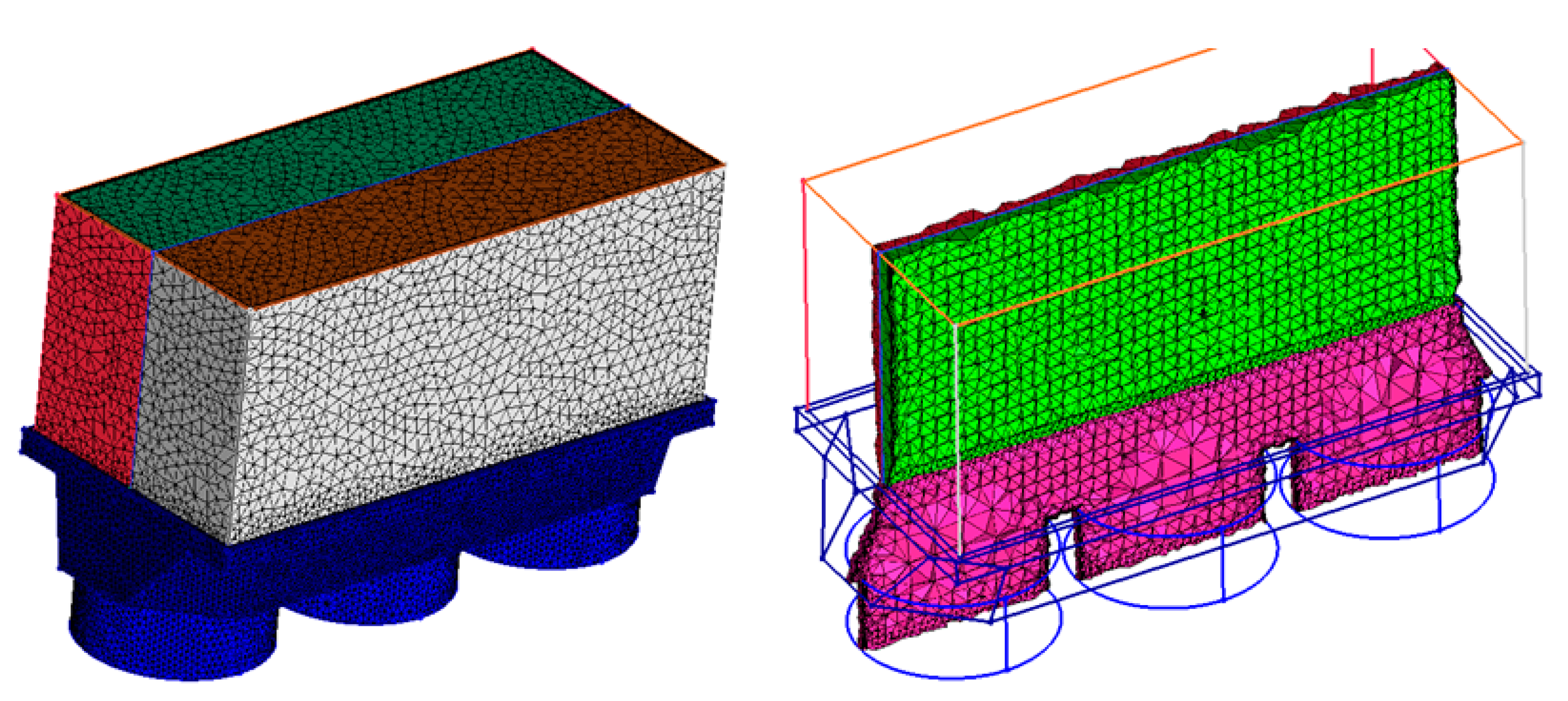
The air-cooled heat exchanger model consisted of three domains. The heat exchange unit was modeled with two parallelepipeds without modeling the real design of the coil bundle. The lower part of the model included units with three fans without modeling the blades. An enlarged computational mesh of tetrahedra was built. The winding radius of the coil was taken as the size of the mesh element. The general view of the calculation mesh of the heat exchanger model is shown in
Figure 6.
Figure 7 shows a diagram of the boundary conditions. At the fan inlets, a function of the total pressure was set as a function of the average flow rate of the air flow that considered the rotational speed. These data were obtained from the aerodynamic characteristics of the fan provided on its technical data sheet.
At the outlet of the heat exchange unit, the boundary condition “Opening” was set, which allowed for the presence of return flows back into the model. On these surfaces, the static pressure was set to 0 Pa (exit to the atmosphere).
The heat exchanger implements a two-pass scheme for the flow of the working medium inside the coils, i.e., the liquid first descends down half of the coils, then collects in a common collector and enters the second half of the coils, where it rises (see
Figure 2 and its description). In this case, the surface temperature of the coils cannot be the same; some of the coils must have a slightly lower temperature since the liquid has already partially cooled in the previous coils. However, in Ansys CFX version 19.0, it is not possible to set the temperature of the porous structure’s solid frame by using a function of the regime parameters. Due to the limitation of the implemented model of a porous body with heat exchange, the temperature of the solid frame can only be set as constant within one porous region. Therefore, the heat exchange unit was divided into two regions. Within each region, the temperature of the solid frame of the porous domain was set to constant and amounted to 55 °C and 50 °C.
In this paper, four regimes of heat exchanger operation were considered; the regimes differed in the number of fans turned on and the speed of blade rotation (
Table 1). When simulating regimes with switched off fans, the boundary conditions for that fan’s inlet were replaced by an “Opening”. In this case, the coefficient of hydraulic resistance of the switched off fan was also set as determined from the its technical data sheet.
4. Results and Discussion
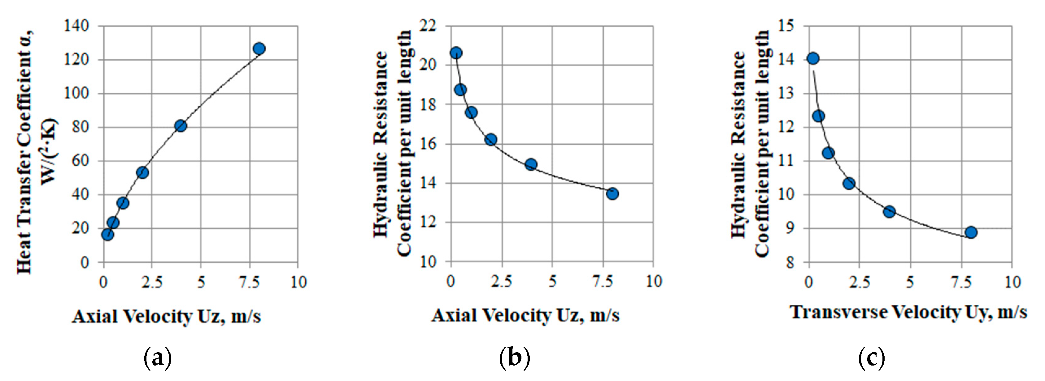
4.1. Closing Relations for a Porous Medium Model
Graphs of dependences of coefficients α,
, and
on air velocity are presented in
Figure 8. The data obtained were approximated by power functions in the considered range of velocities and were subsequently used to describe the characteristics of the heat exchange surface in the porous medium model.
The heat transfer coefficient increased non-linearly with increasing air velocity. Its value changed from 20 to 120 W/m2∙K when changing from the air velocity corresponding to natural convection to the velocity corresponding to forced convection due to the operation of the cooling fans at maximum speed. A decrease in air velocity in this case, for example due to the shutdown of one or more fans, will lead to a decrease in the heat output since part of the heat exchange surface will be cooled inefficiently.
Coefficients of hydraulic resistance per unit length for longitudinal and transverse air flow around the coils are not the same, but their dependences on air velocity are similar. This may indicate that a decrease in air flow which is caused, for example, by turning off the fan will lead to the occurrence of transverse flows inside the heat exchange unit with coils, since both the longitudinal and transverse coefficients of hydraulic resistance increase with a decrease in speed. If the value of the longitudinal resistance coefficient were much lower, then when the fan was turned off, the entire section of the heat exchange surface would be excluded from the heat exchange process since the flow from the operating fans would flow strictly upwards rather than moving in the transverse direction.
4.2. Air Velocity Field in Heat Exchanger
Figure 9 shows the vertical air velocity fields inside the heat exchange unit for different fan operation regimes. The simulation results showed that when all three fans are operating (regimes No.1 and No.2), the air flow in the heat exchange unit is uniform and has the same speed. When operating with the central fan turned off (regime No.3), an unevenness appears in the air velocity profile inside the SBRC bundle, which decreases at approximately half the height of the heat-exchange unit due to transverse overflows between the coils. When operating with two disabled side fans (regime No.4), the unevenness of the velocity profile at the inlet to the heat exchanger increases, but the alignment occurs at one third of the height of the heat exchange unit.
For disabled fans in the calculation, there is a reverse flow of air from the model. This leads to part of the air flow pumped by the switched-on fans not participating in the heat removal; however, energy is still spent on its pumping.
4.3. Air Temperature Field in Heat Exchanger
Figure 10 shows cartograms of the temperature of the air pumped through the heat exchange unit. The air temperature field is uneven when the fans are off. This affects the efficiency of heat transfer, and the magnitude of the heat flux removed.
Based on the calculated data obtained for the air velocity and temperature, the thermal power
Q was calculated, which was removed by air from the surface of the SBRC. The calculation was carried out according to the following formula:
where
G is the mass flow rate of air through the outlet boundary, kg/s;
cp is the heat capacity of air at an average temperature, J/(kg K);
Tout and
Tin are average air temperature at the outlet and inlet boundary, °C.
The results of the calculation are presented in
Table 2. The table also shows the total electrical power consumption of the fans, as determined from their datasheet, depending on the operating point obtained.
5. Discussion
The analysis of the obtained results shows that the maximum thermal power removed by one heat exchanger is about 530 kW at an ambient temperature of 25 °C. This value is achieved in operating mode No.1 (nominal operating mode). The rated thermal power in this mode, as declared by the manufacturer, is 500 kW, which confirms the correctness of the numerical model of the heat exchanger and the coefficients obtained for it.
When the heat exchanger operates in regimes No.2 and No.4, it is possible to divert approximately the same power of 315 ÷ 330 kW; however, for mode No. 2, about 2.7 kW of electricity will be spent, and for mode No. 4, spending 7 kW of electricity is necessary. Thus, when it is necessary to remove less than nominal amounts of power, it is more profitable to work with three fans at low speeds than to turn off individual fans.
6. Conclusions
The paper presents a technique for creating a CFD model of a heat exchanger with close-packed coils in a small bend radius in the approximation of a porous body without detailing the shape of the heat exchange surface. This simplification made it possible to significantly reduce computational costs and computation time.
The main results obtained in this work:
- −
the dependences of the heat transfer and hydraulic resistance coefficients were obtained during the air flow through the annular space of the heat exchanger with the SBRC for different velocities;
- −
the heat transfer coefficient increased non-linearly with increasing air velocity. Its value changed by a factor of 6 when changing from the air velocity corresponding to natural convection to the velocity corresponding to forced convection due to the operation of the cooling fans at maximum speed;
- −
coefficients of hydraulic resistance for longitudinal and transverse air flow around the coils are not the same, but their dependences on air velocity are similar to each other.
- −
on the basis of the created model of the heat exchanger with the use of a porous medium, the fields of air velocity and temperature in the heat exchange unit was studied. When the fans are turned off, these fields become uneven, as a result of which part of the heat exchange surface is inefficiently used in heat transfer.
- −
for the investigated modes of operation, the values of the thermal power removed by the air were determined. For two modes that differ in the number of operating fans and their rotation speed, the same values of the removed thermal power of 315 kW were obtained, however, the consumed electric power was different 2.7 and 7 kW, which affects the cost of operating this equipment.
The created numerical model of the heat exchanger using a series of automated parametric calculations in a reasonable time can be used to create a model of a reduced order. Such a model is a database (or function) with several input arguments, such as ambient temperature, coolant temperature at the inlet and outlet, fan speed.
The implementation of the approach proposed in this article, which is similar to other heat exchange equipment with surface shapes that are difficult to model, will allow the development of digital twins and numerical models. These models can be used to examine various operating modes of both individual elements and entire industrial complexes and facilities. In addition, such models of equipment can be used to develop algorithms for the operation of automated process control systems, which will increase the accuracy of monitoring and maintaining the thermal parameters of the coolant.

 ,
, 


