Article

CFD Study of Thermal Stratification in a Scaled-Down, Toroidal Suppression Pool of Fukushima Daiichi Type BWR

by
Sampath Bharadwaj Kota
1,2,
Seik Mansoor Ali
1 and
Sreenivas Jayanti
2,*
1
Safety Research Institute, Atomic Energy Regulatory Board (AERB), Kalpakkam 603102, India
2
Department of Chemical Engineering, Indian Institute of Technology (IIT)-Madras, Chennai 600036, India
*
Author to whom correspondence should be addressed.
Fluids 2023, 8(1), 20; https://doi.org/10.3390/fluids8010020
Submission received: 13 November 2022 / Revised: 27 December 2022 / Accepted: 28 December 2022 / Published: 4 January 2023

Abstract

:
During the 2011 nuclear catastrophe at Fukushima Daiichi, Unit 3 had a sharper increase in containment pressure than Unit 2, with thermal stratification of the suppression pool cited as one of the contributing factors. In the present work, the buoyancy-induced circulation consequent to steam condensation in a large, toroidal pool of water is studied using computational fluid dynamics (CFD) simulations with a view to understanding the role of important design parameters of the suppression pool system. The tunnelling phenomenon observed in the development of the thermal stratification process is delineated in terms of the establishment of a thermocline. The effects of the number of steam injection points and the cross-section of the pool on thermal stratification characteristics have been investigated through a number of case studies. In all the cases, the surface temperature, which is responsible for over-pressurization of the containment, is found to be significantly higher than the bulk pool temperature. Multiple injection points with the same overall steam flow rate are found to lead to higher surface temperatures due to a shortened circulation path. For the same volume of pool water, the simulations show that a deeper and narrower pool gives rise to significantly higher temperatures than a wider and shallower pool. This is attributed to the relatively deeper penetration of the buoyancy-induced circulation into the pool.

Graphical Abstract

1. Introduction

As part of the defence-in-depth philosophy of ensuring safety, a nuclear reactor is equipped with many barriers to prevent and limit the escape of radioactive fission products in the case of a hypothetical accident. The containment vessel serves as the last line of defence against the leakage of radioactive fission products into the environment. Maintaining the containment’s integrity is of the utmost significance, and numerous designed safety features are included in the reactor for its safety. The suppression pool (SP), which is located inside the containment vessel, provides a means of condensing steam produced by decay heat in an accident scenario and scrubbing fission products carried over by it. It also thereby serves to minimise pressure rise inside the containment vessel.
The Fukushima Daiichi nuclear reactors were impacted by the Great East Japan Earthquake and the tsunami on March 11, 2011. Following this, reactor Units 1–3 (from now on, a nuclear reactor will be referred to as a unit) lost both DC and AC power, triggering a chain of events that culminated in the release of radioactivity into the environment following the breach of the ultimate barrier. During the station blackout transient phase faced by Units 2 and 3, steam was released into the suppression pool through blowdown pipes or spargers of the reactor core isolation and cooling (RCIC) system. The steam vigorously condensed in the suppression pool, transferring its latent heat to the massive water surrounding the blowdown pipe/sparger. Throughout the accident transient, it was noticed that the primary containment vessel (PCV) pressure in Unit 3 was steeper than in Unit 2 during the first twelve hours of RCIC operation [1].
To comprehend the various reasons for the pressure variation, a number of numerical and experimental analyses were conducted. One of the explanations given for the modest pressure increase in Unit 2 was the tsunami-inundated torus chamber [2]. However, the inundation is often modelled as being gradual, reaching its maximum water level around 30 h after the scram [3]. The second explanation was linked to the disparities in the RCIC pipe input in the suppression pool and the duration of operation of the safety relief valves [3]. Although Units 2 and 3 were twin units, Unit 2 had a blowdown pipe with a vertically downward single injection, whilst Unit 3 had a multi-hole sparger leading to horizontal injection. It is hypothesised [3,4] that the horizontal multi-injection sparger was responsible for the temperature stratification in Unit 3.
Recognising the importance of thermal stratification in the suppression pool is essential for reactor safety for several reasons. In the BSAF study, researchers determined that disregarding thermal stratification led to a 160 kPa underestimation of the maximum pressure [1]. During stable thermal stratification, the free surface is at a higher temperature than the water in the bulk pool. Since the partial pressure of steam in the air space corresponds to the vapour pressure of the surface water, the higher surface temperature under thermal stratification results in a higher containment pressure than if the pressure were estimated using the bulk temperature. Moreover, during the stratification, the water at depth may remain substantially more subcooled, and may thus constitute a dead volume of water that does not effectively participate in the heat evacuation process. Consequently, the pool surface temperature may become much higher than anticipated and the containment pressure might dangerously grow, jeopardising the integrity of the containment. Second, under the assumption of a mixed pool, the available net positive suction head (NPSH) for the RCIC pump (placed in the bottom area) would surpass sooner than in a thermally stratified pool [1,5].

2. Literature Review and Objective

Since the Fukushima Daiichi nuclear catastrophe, significant experimental and theoretical research has been conducted on the thermal stratification phenomena in the suppression pools. Experiments on steam condensation in subcooled water have been conducted in various geometrical and operational scenarios, including pool designs and vent pipe configurations. Direct contact condensation (DCC) of steam in subcooled water can be broadly categorised into three regimes: (1) the chugging regime, (2) the jetting regime, and (3) the bubbling regime. It is crucial to remember that the emergence or absence of thermal stratification largely depends on the DCC regime surrounding the vent pipe or sparger. The optimal pool depth is determined based on the prevalent pool parameters, such as pool temperature and steam outflow. Several researchers focused their thermal stratification studies on steam condensation regimes, such as complete condensation in the pipe [6,7,8], chugging [5,7,9,10,11], jetting [12,13,14,15,16] and bubbling [4,17,18,19,20]. The impact of type of condensation regime on the formation and disappearance of thermal stratification has also been a topic of concern. All of the condensation maps have a common qualitative feature: the presence of a stable condensation, in the form of a jet-like structure under conditions of substantial steam mass flow. For very low steam mass flows, condensation is predicted to occur entirely within the vent pipe, where unstable circumstances characterised by cyclic oscillations (i.e., oscillation condensation) and rapid bubble collapse are usual. Several pool layouts have been studied: rectangular [17,18,21,22], the cylindrical pools of the PANDA [23], POOLEX [7,24,25,26], and PUMA [27] facilities, toroidal [4,28], and trapezoidal [11]. Downward injection blowdown pipes [3,17,18,28,29], horizontal injection [11,30], vertical upward injection [31], and multi-hole spargers [3,4] are among the vent pipe configurations that have been studied. Consequently, many factors, including the pool’s internal mixing, the quencher’s design and location, and the pool’s size and shape have all been proposed to have a role in the degree to which stratification occurs and the pressure transient it causes in the SP air space.
In addition, both sub-atmospheric [4,17,18] and above-atmospheric pressure [5,20] tests have been conducted. Jo et al. [4] originally depressurised the torus to 15 kPa (abs) to prevent the torus from being pressured due to the temperature rise and to reduce the duration of the experiment. Solom and Kirkland [5] evaluated stratification in the TAMU suppression pool and noticed that when the pool was vented to the outdoors, vertical thermal stratification was limited to 21 °C, but a closed airspace resulted in stratification at over 60 °C. Liu et al. [20] found that thermal stratification increased with vessel pressure under the same steam mass flux condition in a cylindrical tank with varying mass flux (1–3 bar). In addition, they developed a correlation for the dimensionless thermocline down velocity as a function of the Richardson number.
Using system-level codes to represent the whole reactor behaviour to the initiating event, a number of research efforts into thermal stratification have been conducted [6,8,29]. Codes such as MELCOR, TRACE and RELAP5 (except for GOTHIC) assume a well-mixed/homogenous pool [6]. Li et al. [29] used GOTHIC with the effective heat source (EHS) and effective momentum source (EMS) models to simulate thermal stratification and mixing. Their computational models quantified the pool’s transient behaviour and found that the predicted average temperature and water level in the pool agreed with their experiments. Cavaluzzi et al. [6] developed a stratified wet well model using the RELAP-7 code for a complete steam condensation blowdown pipe scenario. They presumed a buoyant plume transferred heat and mass from the steam injection site to the overlying water zone slowly with limited momentum and established that the flow structure resulting from steam injection and condensation at low mass flux could be described by a pure buoyant plume model. Gallego-Marcos et al. [8] employed enhanced EHS/EMS models in the GOTHIC code to simulate steam injection through blowdown pipes in low-steam-mass-flow regimes. They constructed scaled correlations to determine chugging momentum and anticipate condensation transitions.
Moreover, several researchers have conducted numerical investigations with computational fluid dynamics (CFD) tools wherein fluid motion and allied phenomena such as turbulence, heat and mass transfer, and chemical reactions are resolved over a fine scale, both spatially and temporally. Pioneering work in this field was accomplished via the SCR approach [13,14]. Kang and Song [13] considered an axisymmetric CFD design and compared simulated predictions to B and C test results. They conducted a 30-second numerical study for a thermal mixing experiment using the SCR model for steam jet condensation for a multi-hole sparger. Comparing the CFD findings to the test data revealed a satisfactory agreement within a variation range of 7–8% and attributed the disparity between the temperature and velocity of condensed water in the SCR model to that of actual values. Moon et al. [14] utilised the SCR model to study IRWST thermal mixing using CFD simulations and found that there is a significant disparity in temperature profiles near the sparger; however, away from the sparger, temperature increase patterns approximated the experiment.
In addition, reduced-scale 3D CFD simulations were conducted utilising the effective heat/momentum source (EHS/EMS) approach [11,32] or the two-phase Eulerian method [11]. Gallego-Marcos et al. [32] augmented the EHS/EMS model capabilities to include steam injection via multi-hole spargers and calibrated the model against the spargers test conducted in the PPOOLEX and PANDA facilities. They also presented CFD modelling recommendations for realistic pool simulation and a unique relationship to represent buoyancy-caused turbulence generation and dissipation. Their analysis showed that turbulence, not mean shear flow, degrades the cold stratified layer. Qu et al. [11] predicted the temperature distribution inside a 1/400th scaled-down suppression pool of ESBWR using the effective source (ES) approach and the direct contact condensation (DCC) method. They examined fluid velocity distribution and discovered that stratification might be prevented by relocating the injection position downward. They suggested that both approaches could detect thermal stratification in the pool, but only the DCC method could detect the transition between mixing and stratification.
In addition, research [21,33] has demonstrated the influence of non-condensable gas on the development and erosion of thermal stratification. Cai et al. [21] investigated the influence of non-condensable gas (0–24%) on thermal stratification in a rectangular slab-shaped suppression pool. They discovered that nitrogen eliminated thermal stratification in the suppression pool and a higher nitrogen mass flow rate did so quicker. Li et al. [33] observed that air accelerated and worsened thermal stratification below 4% air mass fraction but stopped it beyond 4%.
Further, this form of DCC of steam in the vast pool is not exclusive to Fukushima Daiichi-type boiling water reactors (BWRs). It is also found in other reactors, such as the SP of economic simplified boiling water reactors (ESBWRs), in-containment refuelling water storage tanks (IRWST) in advanced pressurised water reactors (APWRs) [13], and gravity-driven water pools (GDWP) in advanced pressurised heavy reactors (AHWR) [22], for catering to the needs mentioned above.
The thermal stratification transient in the suppression pool generally happens over a long period. During this later phase of this blowdown transient, the steam mass efflux from the vent pipes would have reduced significantly [34]. Therefore, it can be assumed that negligible momentum is introduced into the pool at low steam mass flow rates, and the flow’s source can be considered as buoyancy dominant [6]. Further, even though the steam condensation imparts a little momentum to the suppression pool in the circumferential direction, in the present study, it is assumed that it has an insignificant effect on thermal stratification that is generally expected in the vertical direction.
Further, the available literature on the CFD studies of thermal stratification of suppression pools is mainly for cylindrical/rectangular geometries and does not accurately represent the actual torus-shaped suppression pool present in the Fukushima Daiichi reactor. Further, most of the literature discusses research findings considering forced convection effects during steam injection. However, in the present study, the momentum source is neglected, and only the effect of natural convection during the formation of thermal stratification is considered, which should be valid for low-steam-flux conditions. Thus, in the present study, a reduced-scale whole torus is considered for CFD simulations, and the parametric influence of geometrical and operating conditions on the thermal stratification characteristics of the suppression pool are discussed in this paper.

3. Numerical Modelling

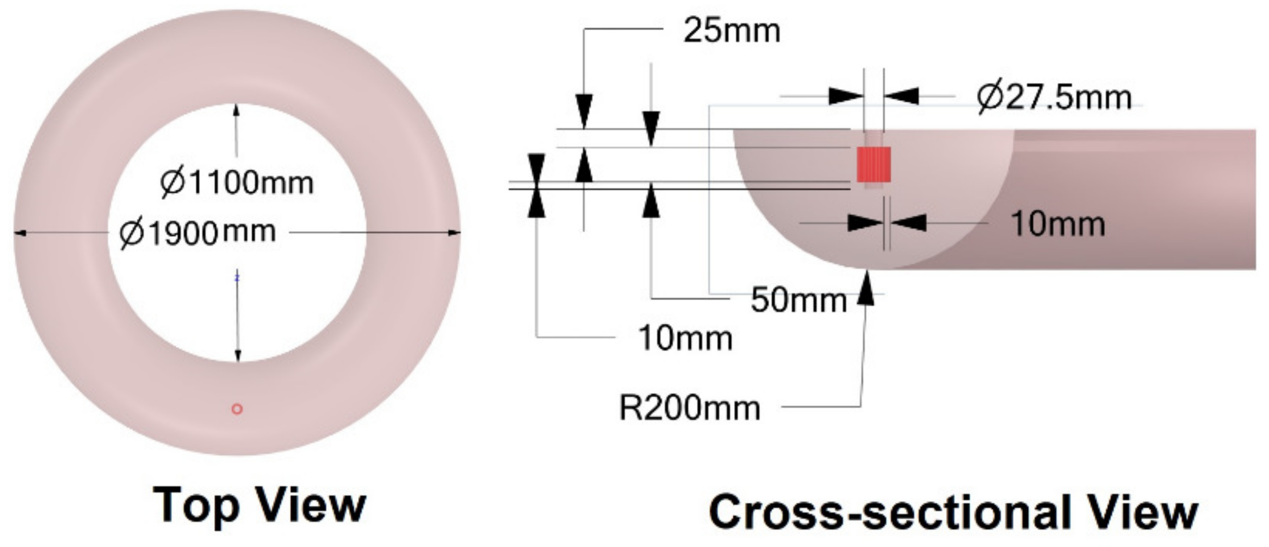
3.1. Geometry Description

The Fukushima Daiichi is a BWR with Mark 1 containment, which consists of a drywell resembling an inverted lightbulb and a toroidal suppression pool chamber. The suppression pool has an inventory of 2980 m3 with a major diameter of 33.5 m and a minor diameter of 8.9 m. The reduced-scale torus has a main diameter of 1.5 m and a minor diameter of 0.4 m, with a volume of 0.592 m3 when half-filled with water. The current study employs the scaled-down suppression pool shape described in the literature [4]. The dimensions of the torus and steam condensation region (SCR) in this study are shown in Figure 1. In addition, a list of simulations performed in this study is provided in Table 1 as a simulation matrix.

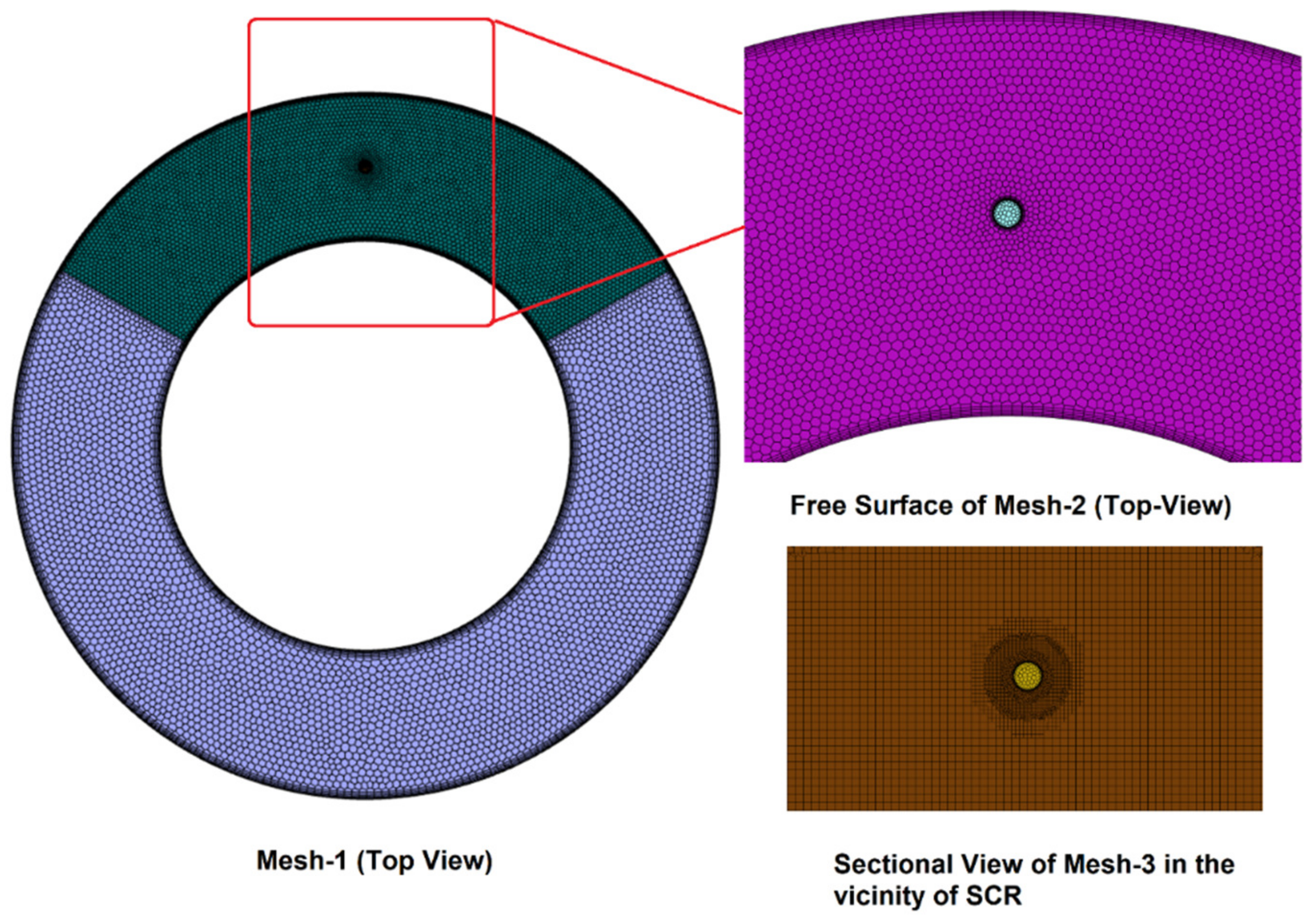
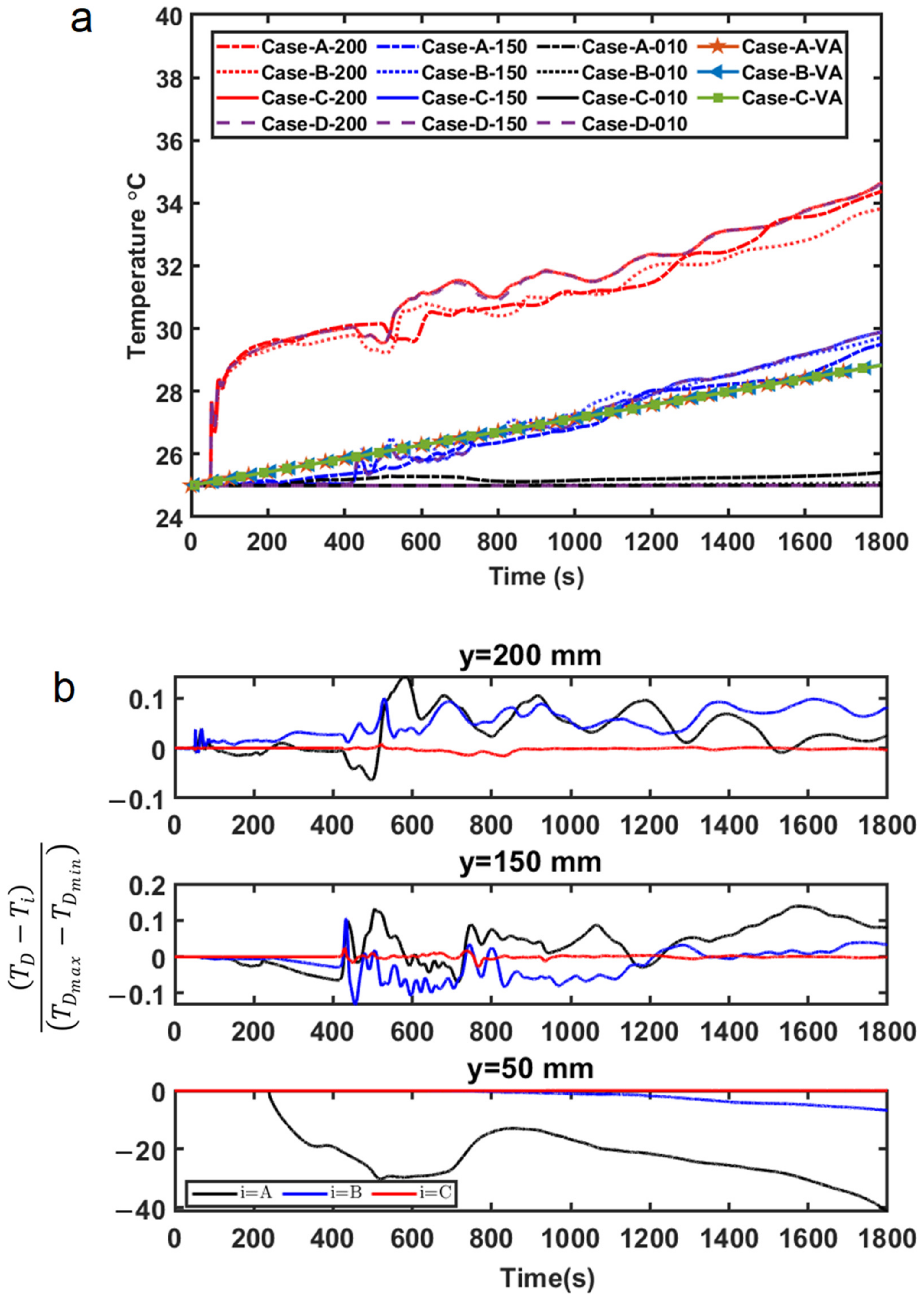
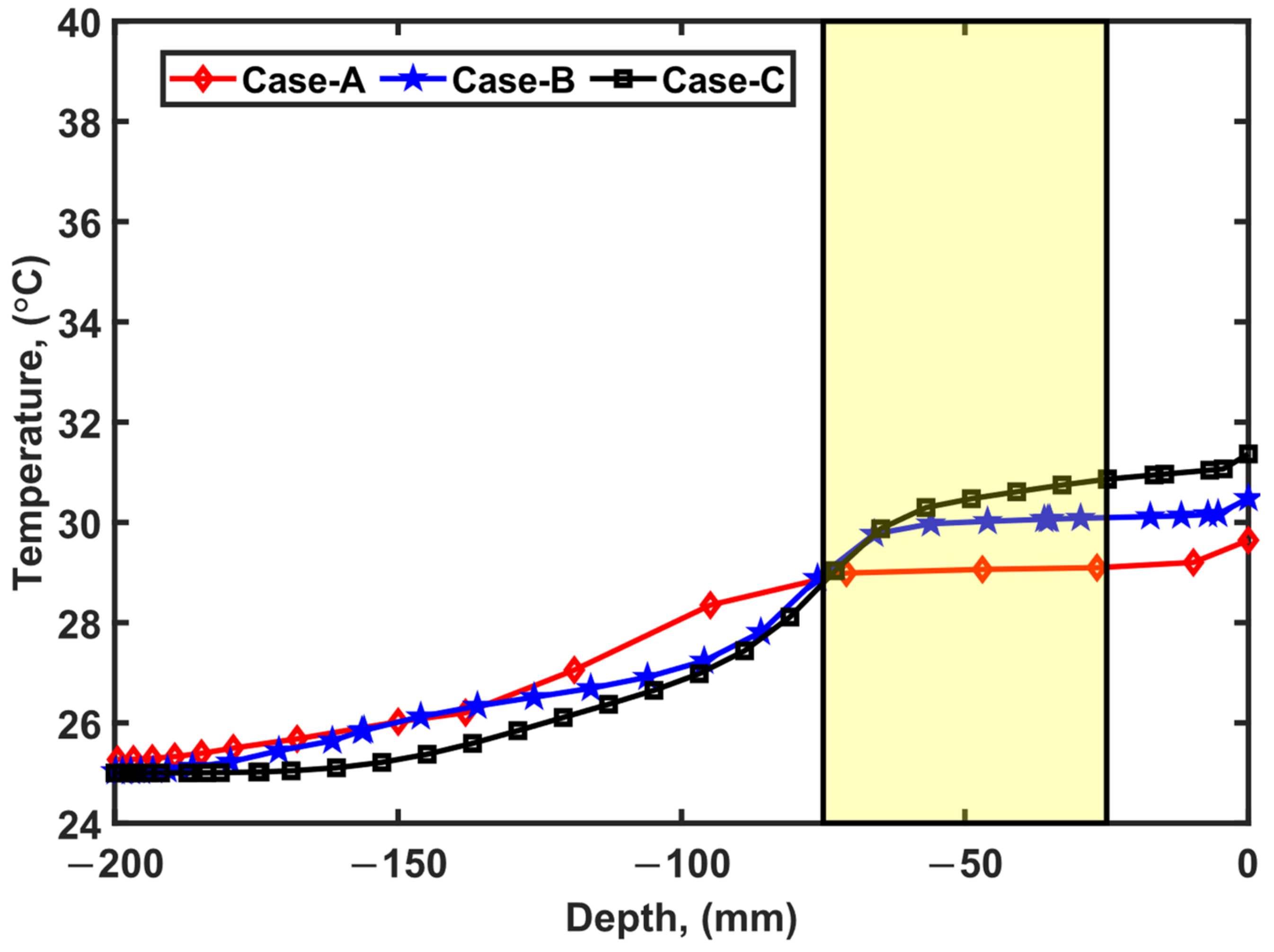
3.2. Case Set-Up and Mesh Sensitivity Study
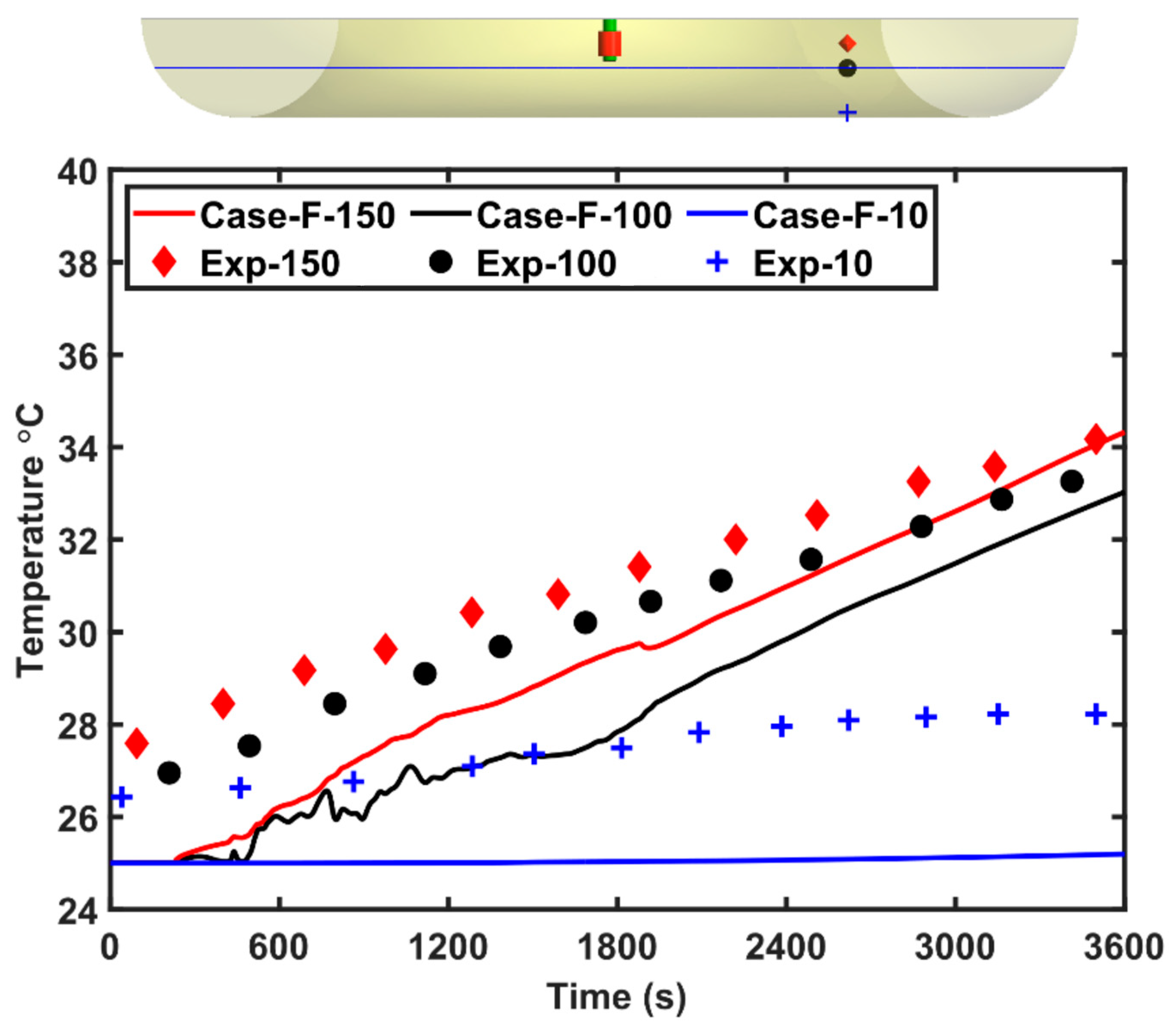
In this investigation, simulations of thermal stratification were conducted using the effective heat source (EHS) approach [7]. The EHS model was applied by introducing a volumetric heat source of 42 MW/m3 as a single source equal to the latent heat of steam condensation in the pool at a flow rate of 3.7 kg/hr. In addition, it was considered that steam condenses instantly in the proximity of the sparger, and the zone where steam entirely condenses is referred to as the steam condensation region (SCR) [7,14,32].
Using the ANSYS mosaic meshing tool, a mesh dominated by hexahedral elements, thus having fewer faces and higher-quality cells, was generated. A study of grid independence was carried out using meshes of 196,000, 512,000, and 930,000 cells with a 25 mm steam penetration length. Typical meshes employed in the present study are given in Figure 2.
The average cell size in the SCR area is 5 mm for coarse mesh and 2 mm for fine mesh. Further, the torus area has an average cell size of 10 mm in a zone encompassing one-third of the sparger and 20 mm in the remaining two-thirds with the coarser mesh (case A), 10 mm for the medium mesh (case B), and 8 mm for the fine mesh (case C). All meshes maintained a minimum orthogonal cell quality of 0.5; for case C, over 99.8% and 97.9% of the cells had an orthogonal cell quality of above 0.8 and 0.9, respectively. In addition, the maximum observed skewness was 0.49, and 99.9% of the cells had skewness less than 0.3.
Figure 3 and Figure 4 summarise simulation results used to study the effect of grid size and time step size (Cases A to D of Table 1) on the predicted temperature variation at selected points in the suppression pool. Figure 3a shows the variation with time in the pool temperature at three locations (at heights of 200 mm (above the SCR), 150 mm (inside the SCR), and 10 mm (below the SCR)); these points are placed 45 degrees counter-clockwise from the sparger’s location) for different mesh and time step sizes. It can be seen that the temperature evolution is substantially different at these three locations, and that the predictions from different grids match very well over the first 300 s. Although there are minor differences, the predictions over 1800 s show very similar dynamics at the three locations. Figure 3b displays the predicted temperature variation in various grids relative to the finest grid (case D) at three sites for various heights, namely 10 mm, 150 mm, and 200 mm. As the grid is made finer, the relative temperature fluctuation (non-dimensionalised by the maximum temperature variation predicted using the finest grid) is shown to decline to less than 0.1 as time approaches 1800 s. Additionally, Figure 4 shows the predicted thermocline at 1600 s. The temperature gradient on the line located diametrically opposite the steam condensation zone ranged from 0.0232 to 0.0318 °C/mm as the mesh size became finer, and the surface temperature differential was around 1.7 °C. In addition, previous CFD research [32] on thermal stratification showed that a 12 mm cell size did not enhance simulation results compared to 25 mm and 50 mm cells. Consequently, it appeared prudent to continue subsequent computations with 930,000 cells (with an average cell size of 8 mm), as any increase in the cell count would increase computational cost drastically with only a marginal improvement in the predictions.
For ascertaining the effect of time step, initially, a time step of 0.01 s was chosen for up to 900 s, 0.05 s for 900 < t < 1000 s, and 0.1 s for 1000 < t < 1800 s for cases A–C. On a system with eight cores and 128 GB of RAM, the simulation for a fine mesh took around 10 days to complete. Later, a simulation (case D) was entirely run using a time step of 0.1 s. Using a constant time-step (case D) of 0.1 s does not influence the observed temperature variation as observed in Figure 3a; thus, a time step of 0.1 s was adopted for subsequent simulations.
Further simulations were also carried out to ascertain the effect of SCR penetration length. For the sake of simplicity, the control volume of SCR was considered to be cylindrical [14], and the initial simulation was carried out with SCR extending up to 25 mm in the radial direction. For the same steam flow rate, decreasing the volume of SCR would increase the volumetric heat generation rate. As the volumetric heat flux did not increase the temperature to unreal levels for a penetration length of 25 mm, a final value of 10 was used to represent the realistic size of the steam condensation zone. It is seen from Figure 5 that the average surface temperature has hardly changed with varying penetration length, whereas the estimated pool bulk temperature, as may be expected, is the same in all three cases. As discussed in the literature [34], the macro-scale phenomena (i.e., pool dynamics such as thermal stratification) depend on available pool volume, the submergence depth of the sparger, and steam influx, and may not be much influenced by meso (i.e., sparger) and micro (jet structure) scale phenomena. In addition, an SCR size of 10 mm is a plausible assumption given that the bubble size in the investigations [4] ranged from 2 to 10 mm and a previous CFD research [12] employed the penetration length as seven times the injection diameter.
The governing equations of continuity, momentum, energy, and turbulent equations are given in Equations (1)–(5), respectively. Equation (1) indicates mass conservation, and momentum conservation is expressed by Equation (2), where p is the static pressure, τ ¯ ¯ is the stress tensor, and ρ g and F are the gravitational and external body forces, respectively. Additionally, the energy equation is provided by Equation (3), and the first two components on the right-hand side of Equation (3) reflect, respectively, energy transfer owing to conduction and viscous dissipation. In addition, S h signifies the volumetric heat source resulting from steam condensation in the area around the sparger. Further, this work uses the standard k-ε turbulence model to compute turbulent length and time scales. It relies on model transport equations for turbulence’s kinetic energy (k) and dissipation rate (ε). The model’s equations were developed utilising phenomenological concepts and empirical data. This turbulent model is accurate, computationally efficient, and adaptable to diverse turbulent flows. In these equations, G k and G b signify the creation of turbulent kinetic energy due to the mean velocity gradients and buoyancy-induced turbulence. Additionally, in compressible turbulence, Y M represents the contribution of variable dilatation to the overall dissipation rate. The default values of 1.44 and 1.92 are employed for model constants C 1 ϵ and C 2 ϵ , respectively.
This study implements the following boundary conditions: The torus and sparger outer walls are considered adiabatic walls with enforced no-slip boundary conditions. In addition, the free surface of the torus is assumed to be a zero-shear wall with a convective heat transfer coefficient of 4 W/m2C and exposed to an ambient temperature of 45 °C. In addition, the heat production owing to steam condensation close to the sparger is imposed as the volumetric heat flux in the steam condensation region (SCR).
The SIMPLE technique was utilised for solving pressure–velocity coupling in Ansys Fluent [35]. The pressure and velocity are updated consecutively in this method, which is of the segregated kind. In addition, second-order spatial discretisation schemes were utilised for the pressure, momentum, turbulence and energy equations, and a second-order implicit scheme was for the transient formulation. Except for the energy equation, all equations (continuity, momentum, turbulence) were regarded as fully converged when the total of scaled residuals was less than 10−5 and for energy when the sum of scaled residuals was less than 10−8. The water properties used in the simulation are listed in Table 2.
ρ t + . ( ρ v ) = 0
( ρ v ) t + . ( ρ v v ) = p + . ( μ τ ¯ ¯ ) + ρ g + F
t ( ρ ( e + v 2 2 ) ) + . ( ρ v ( h + v 2 2 ) ) = . ( k e f f T + τ = i j . v ) + S h
( ρ k ) t + . ( ρ v k ) = . ( Γ k k ) + G k + G b ρ ϵ Y M + S k
( ρ ϵ ) t + . ( ρ v ϵ ) = . ( Γ ω ϵ ) + C 1 ϵ ϵ k ( G k + C 3 ϵ G b ) C 2 ϵ ρ ϵ 2 k + S ϵ
The variation in density with temperature was modelled using the Boussinesq approximation as shown in Equation (6). This assumption is based on the fact that, even though the temperature-induced density change is small, the density fluctuation is strong enough to generate buoyant motion. With the exception of the buoyancy factor in the momentum equation, the fluctuation in density is thus disregarded everywhere. The Boussinesq approximation is valid if | β ( T T r e f ) | 1 .
ρ = ρ r e f ( 1 β Δ T )

3.3. Validation

The current work has been validated in light of the tunnelling behaviour exhibited in the suppression pools [4,34,36,37], which is discussed in detail in the following section. The current analysis focuses on comparison with the measured time-dependent temperature variation at TT1 locations [4]. The predicted temporal variation in temperature at a location inside the SCR plane, one directly below the SCR, and one far away from the SCR are compared with experimental data [4] in Figure 6. As per predictions, at around 230 s, the temperature rises dramatically at points located at heights (from the bottom) of 150 mm and 100 mm, which may be ascribed to the hot, buoyant plume propagating over the torus and reaching the points at these locations. The temperature at the distant location with a height of 10 mm from the bottom does not exhibit this rise and stays virtually constant. Further, by the late time of 1800 s, as will be shown later, the flow pattern is usually stabilised, and the subsequent temperature change at a given place is nearly linear. The comparison of the predicted variation with experimental data in Figure 6 shows a good qualitative trend at all the three locations. There is some discrepancy in the quantitative values. The following points may account for the difference between experiments and simulations: firstly, the specific coordinates of TT1 sites are unknown; in Figure 6, the comparison is made for a point located at 45° circumferentially relative to the mid-plane of the volumetric heat source. Secondly, in the experiments, the initial bulk temperature was not uniform, and had a temperature variation in the order of 1.5 °C, with the lowest temperature in the pool being 25.7 °C. In the present study, a constant initial pool temperature of 25 °C is assumed. These differences may account substantially for the quantitative differences between experimental data and the simulated data. This is further substantiated by a comparison of the predicted and measured rates of increase in temperature at different locations. As can be seen in Table 3, there is very good agreement in all the three cases, showing the essential dynamics are captured sufficiently accurately.

4. Results and Discussion

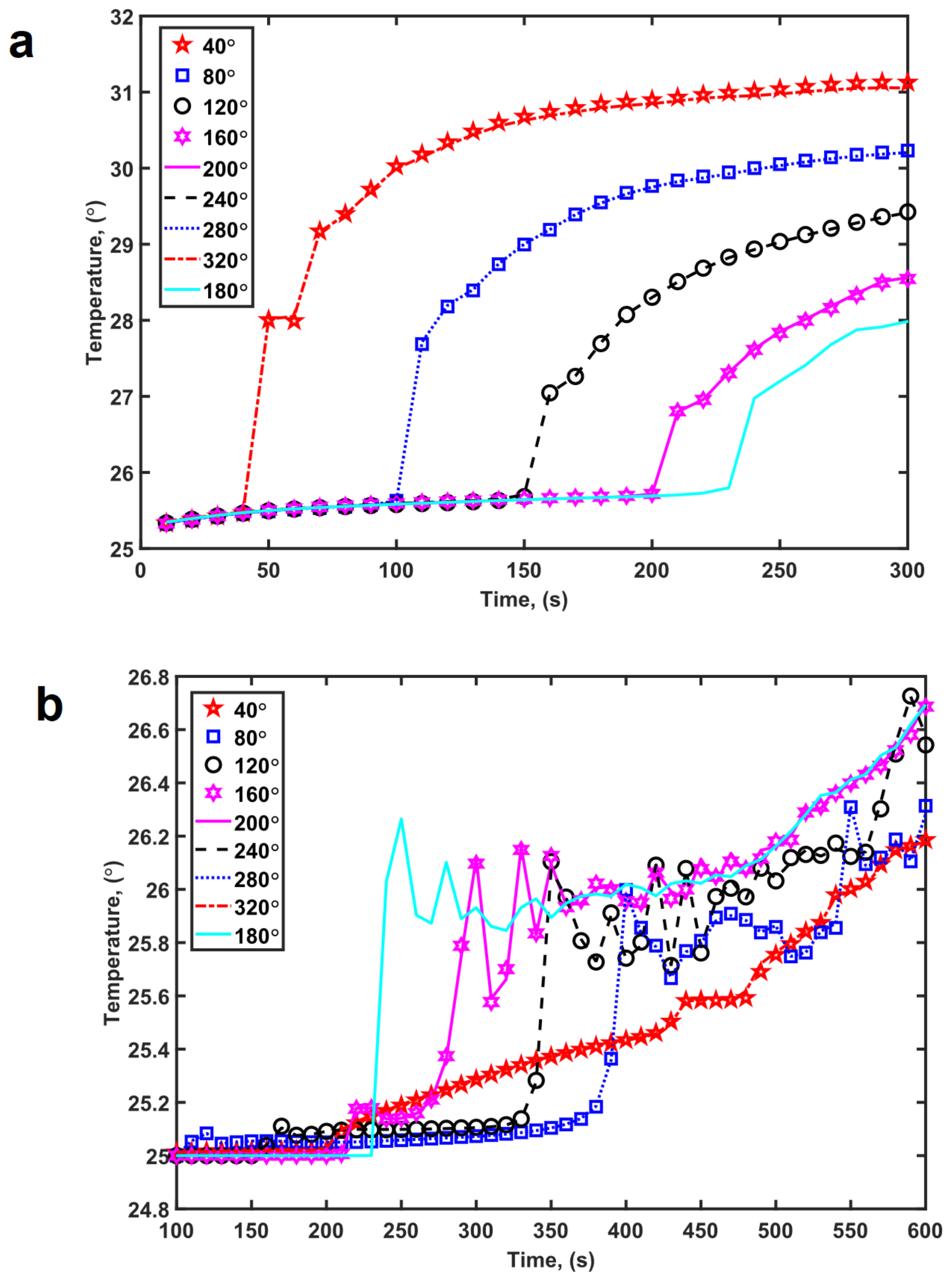
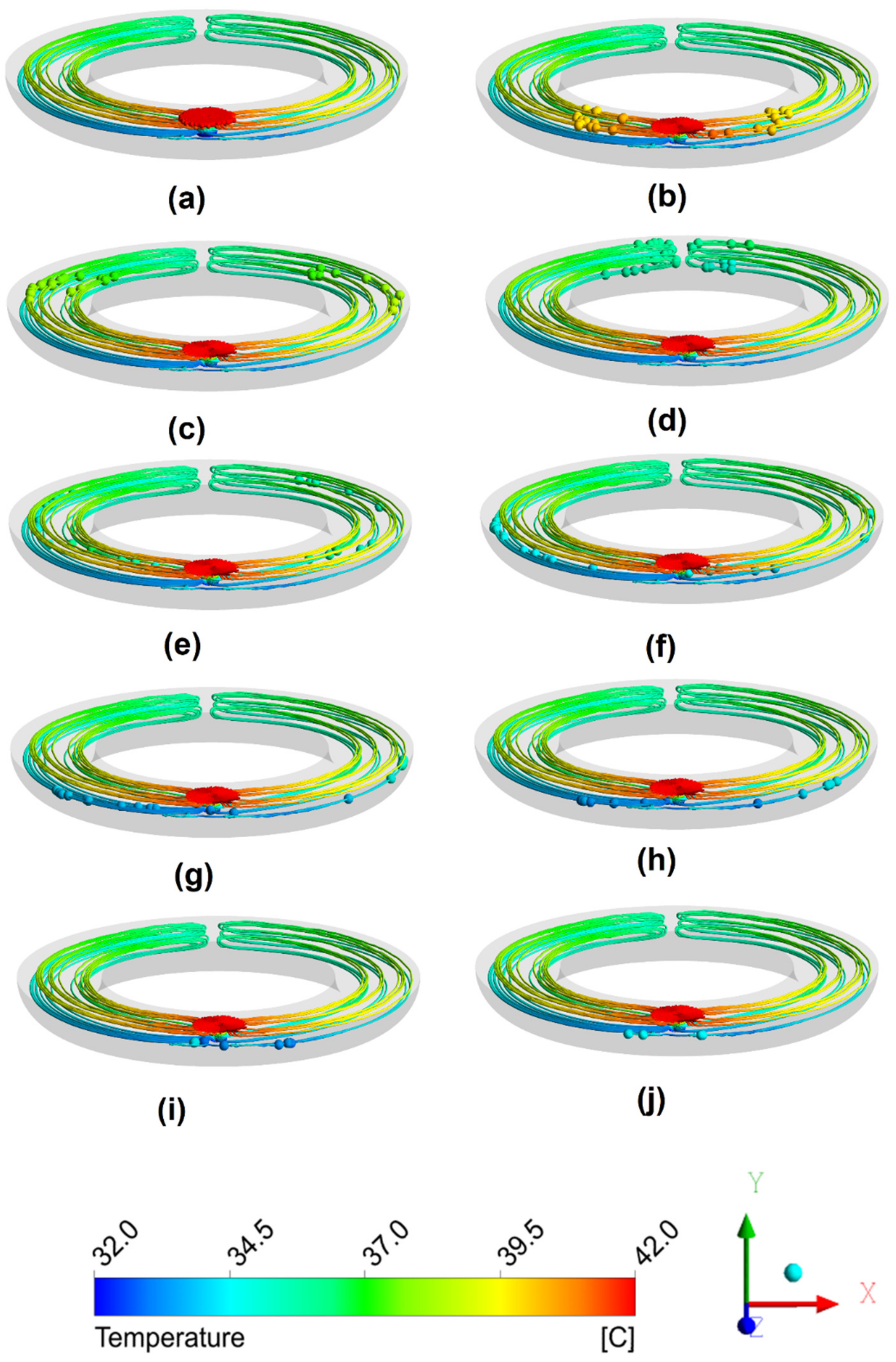
4.1. Tunnelling Effect

Due to volumetric heat generation equal to the rate of release of latent heat from condensation of steam in the vicinity of the sparger (SCR), the water in the SCR is warmer than the surrounding water. This temperature differential causes buoyant plumes to rise to the pool’s surface from the SCR. Once the heated plume reaches the top free surface, it spreads circumferentially in clockwise and counter-clockwise directions around the torus until it reaches the other end. The temporal variations in temperature at points located circumferentially on the surface and 50 mm below the surface are shown in Figure 7a and Figure 7b, respectively. As and when the hot front reaches a particular location, there is an instant spike in temperature. As seen in Figure 7a, the fronts intersect around 230 s in a place diametrically opposite the heat source. This event is characteristic of the chimney/tunnelling effect, as reported in the literature [37]. While the thermal fronts continue to propagate circumferentially, the plume transfers heat to the surrounding cold water before their collision, as seen in Figure 7a, and moves towards the sparger at a lower altitude, as seen in Figure 7b. At a depth of 50 mm, there is hardly any rise in temperature until 230 s, but, immediately after the fronts’ collision, the temperature sharply rises at 180°, indicating the front is moving downwards. As time progresses, it is seen that the temperature rises at the sites (in the temporal sequence of 180°, 160°and 200°, 120° and 240°, 80° and 280°) as the thermal plume approaches the sparger, suggesting that the colder plume is returning to the sparger and a flow pattern is being established.
The streamlines determine the observed circulation pattern during the transient simulation when a stable flow pattern emerges. In addition to identifying the pool’s temperature, the streamlines comprise markers indicating the direction of movement. In summary, the facets of the tunnelling phenomenon consist of a heated plume rising from the region of the sparger (Figure 8a), expanding circumferentially (Figure 8b,c), sinking at the opposite ends of the sparger (Figure 8d), and returning to the sparger at a lower height (Figure 8e–j). Even though this is a basic description, the established flow pattern is more complicated, with several recirculation patterns and stagnant zones.

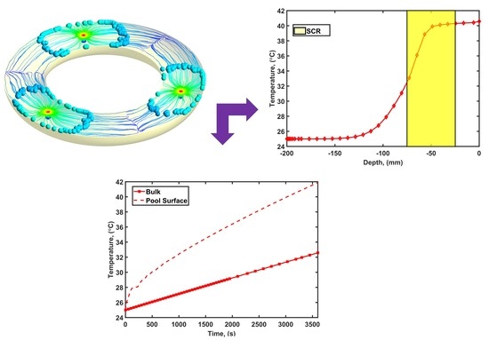
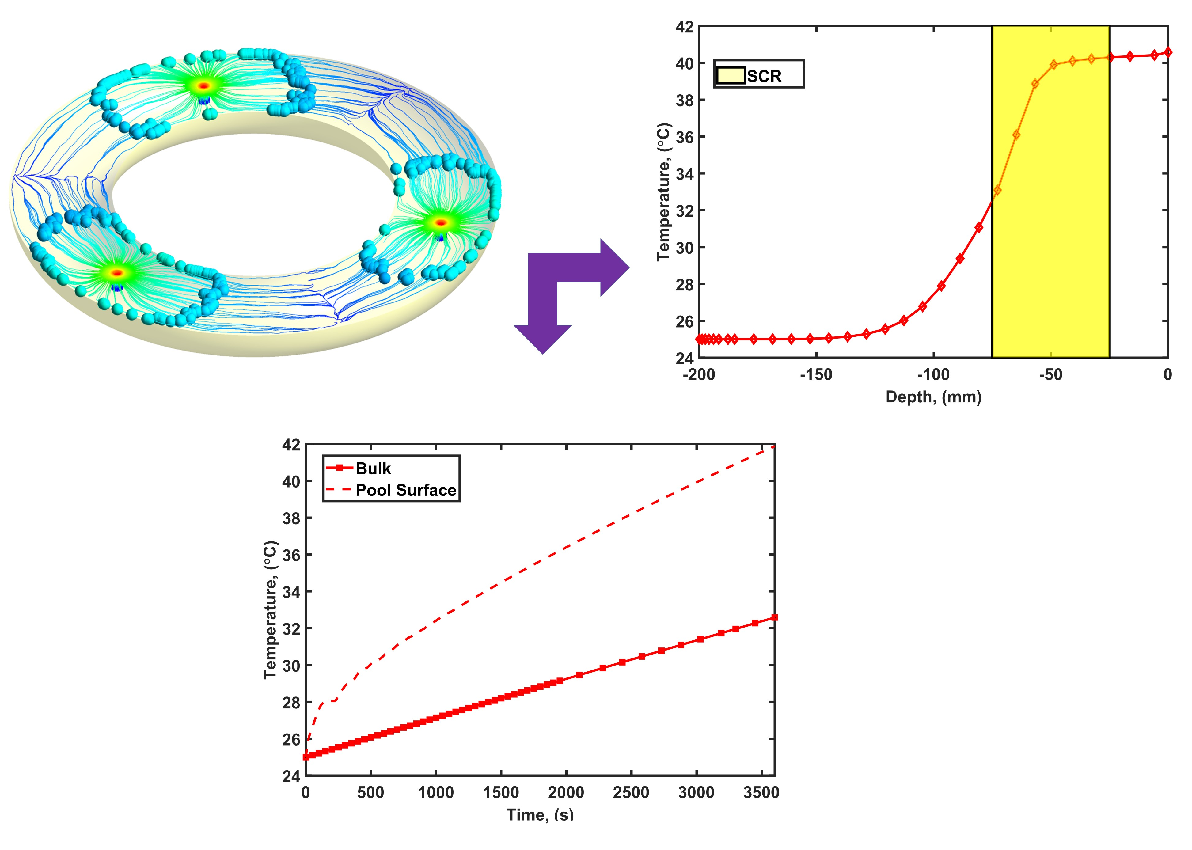
4.2. Thermal Stratification Characteristics for Base Case

The thermal stratification characteristics for the base case, i.e., case F, have been published earlier [38], and for easy reference these results are paraphrased in this study.

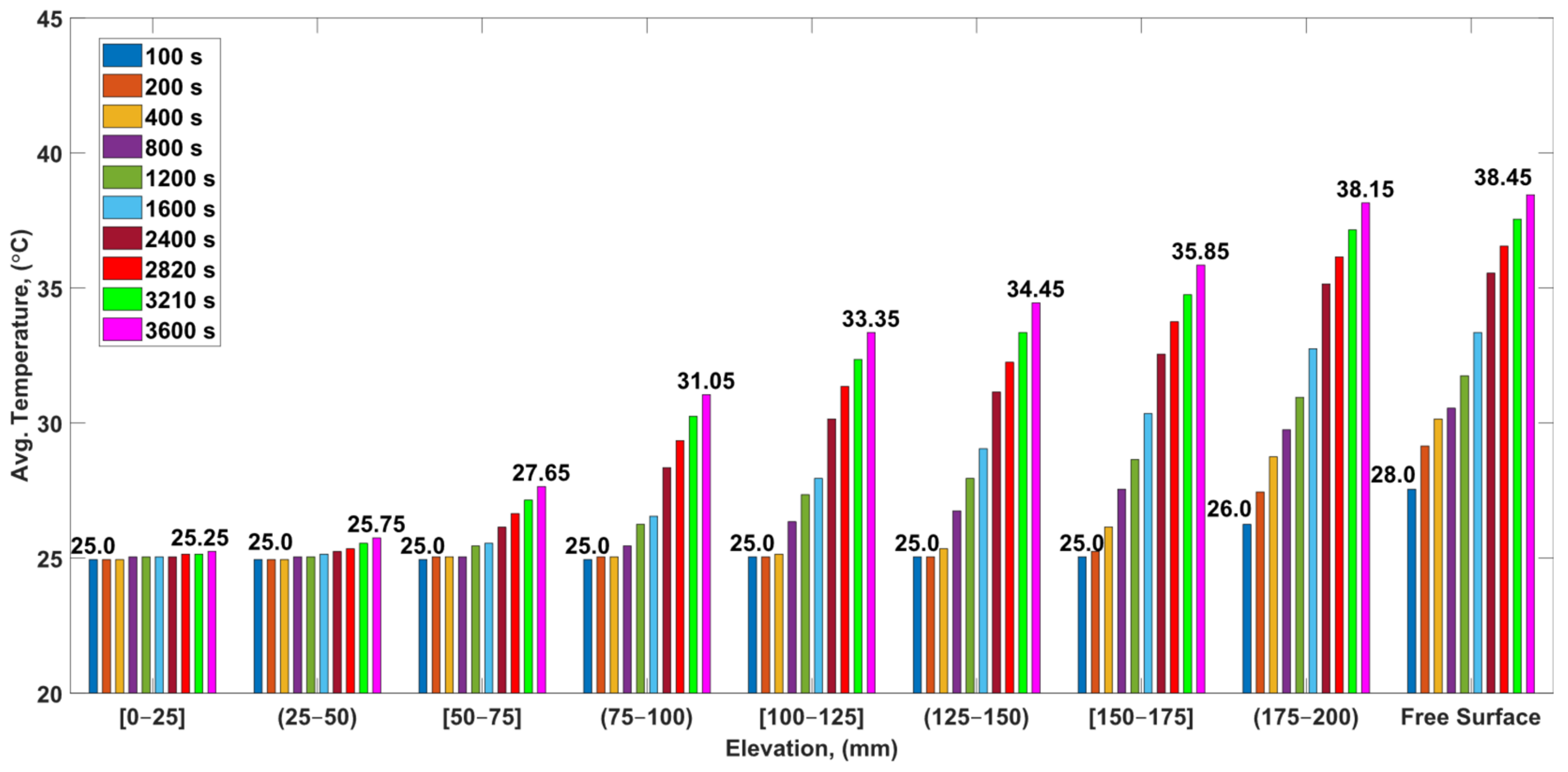
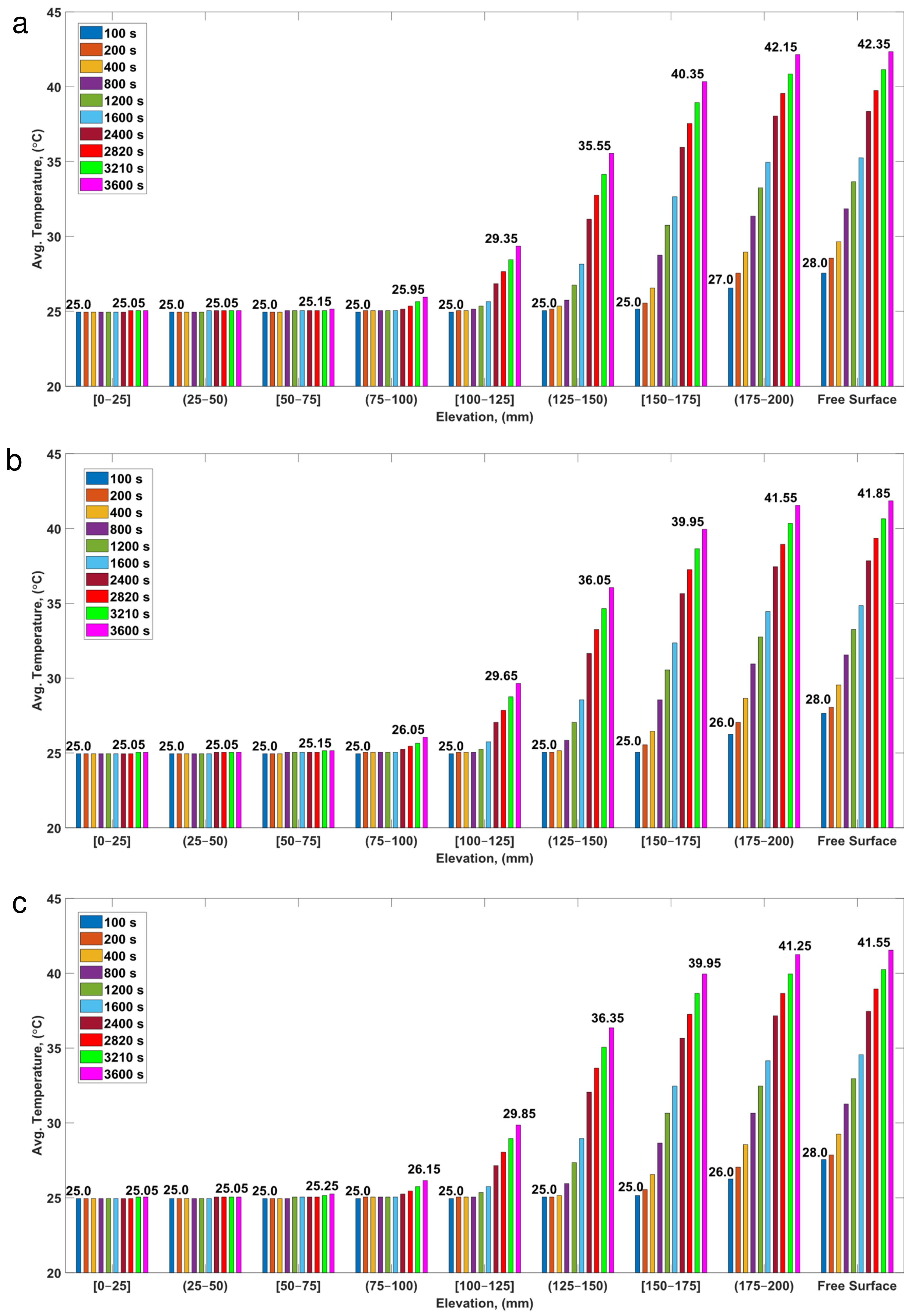
4.2.1. Average Temperature Distribution

Figure 9 depicts the average temperature distribution in the pool with regard to elevation at different times. Throughout the 3600 s, the bottom-most zone, i.e., from 0 to 25 mm in elevation, saw just a 0.25 °C rise. This shows that the zone is not evacuating heat during the buoyancy-induced convection process and might be deemed a stagnant zone. In the highest zone, however, the temperature fluctuation is 13.15 °C, showing that this zone actively participates in the circulation process. In addition, if the initial pool temperature of 25 °C is considered, the surface temperature rose by 13.45 °C during the same period. The dead volume can be defined in terms of the temperature rise that it has undergone. If it is defined as the zone with less than a 20% rise in temperature (ΔT = 13.45 × 0.2 ≈ 2.7 °C) relative to the highest temperature difference (seen for free surface: ΔT ≈ 13.5 °C), the dead volume may be detected up to an elevation of 0–75 mm during the allotted period. (It may be noted that 2.7 °C corresponds to about 35% of the well-mixed temperature rise and, thus, even in terms of the average amount of heating up, the dead volume constitutes a considerable thermal inertia.) This dead volume represents about 35% of the pool’s overall volume. In addition, a considerable temperature change is detected in the zones between 75 and 200 mm, suggesting mixing.

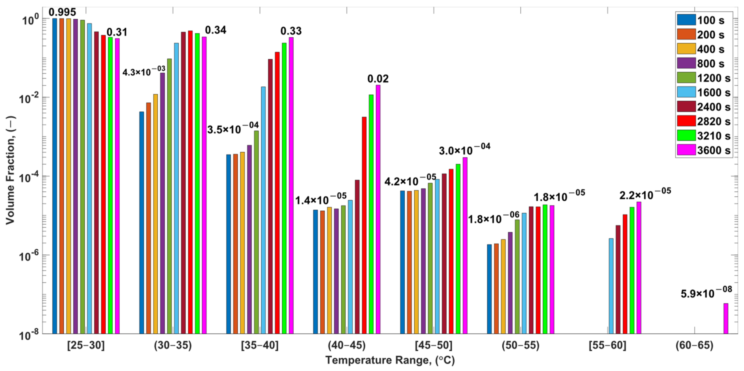
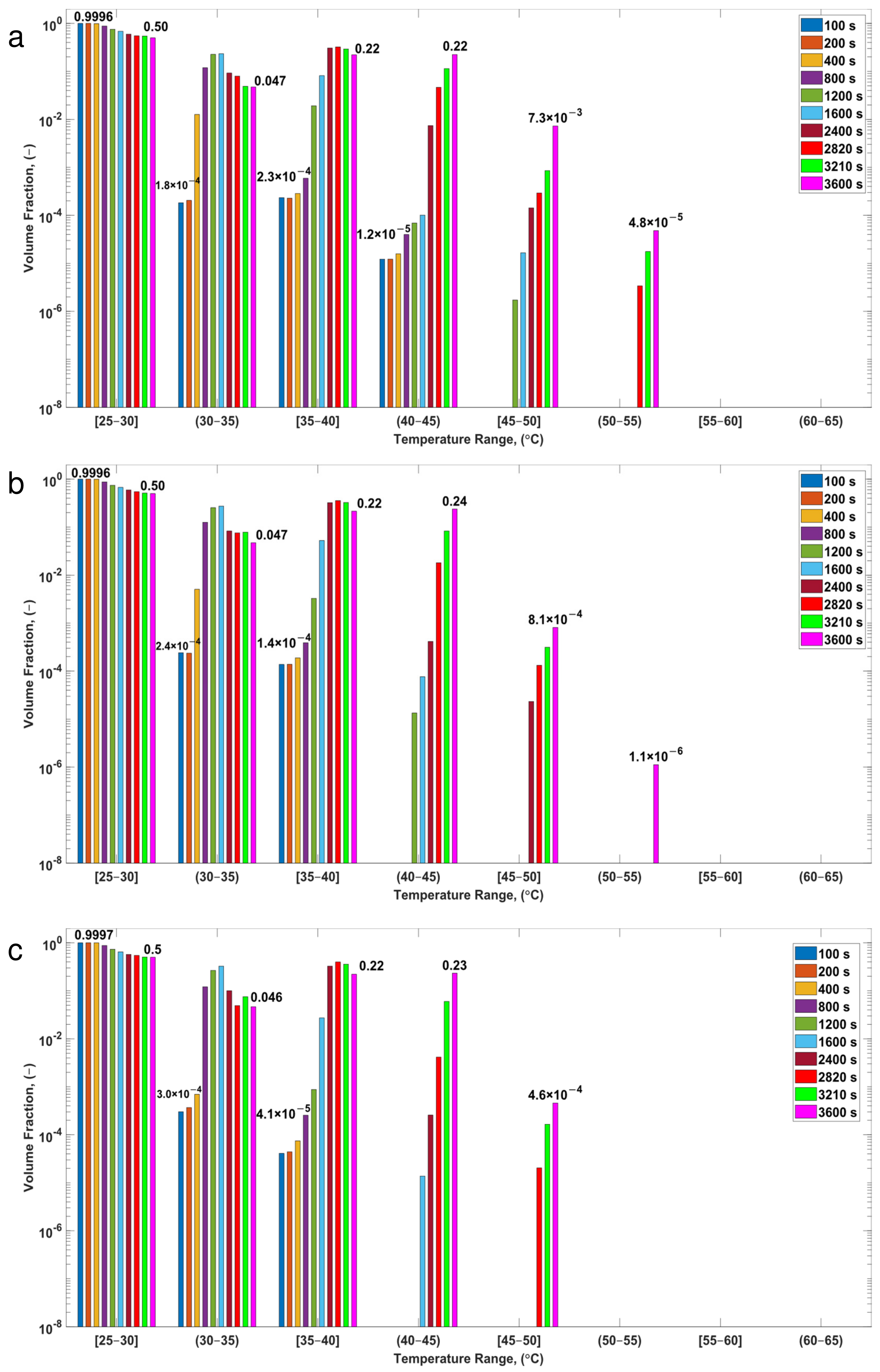
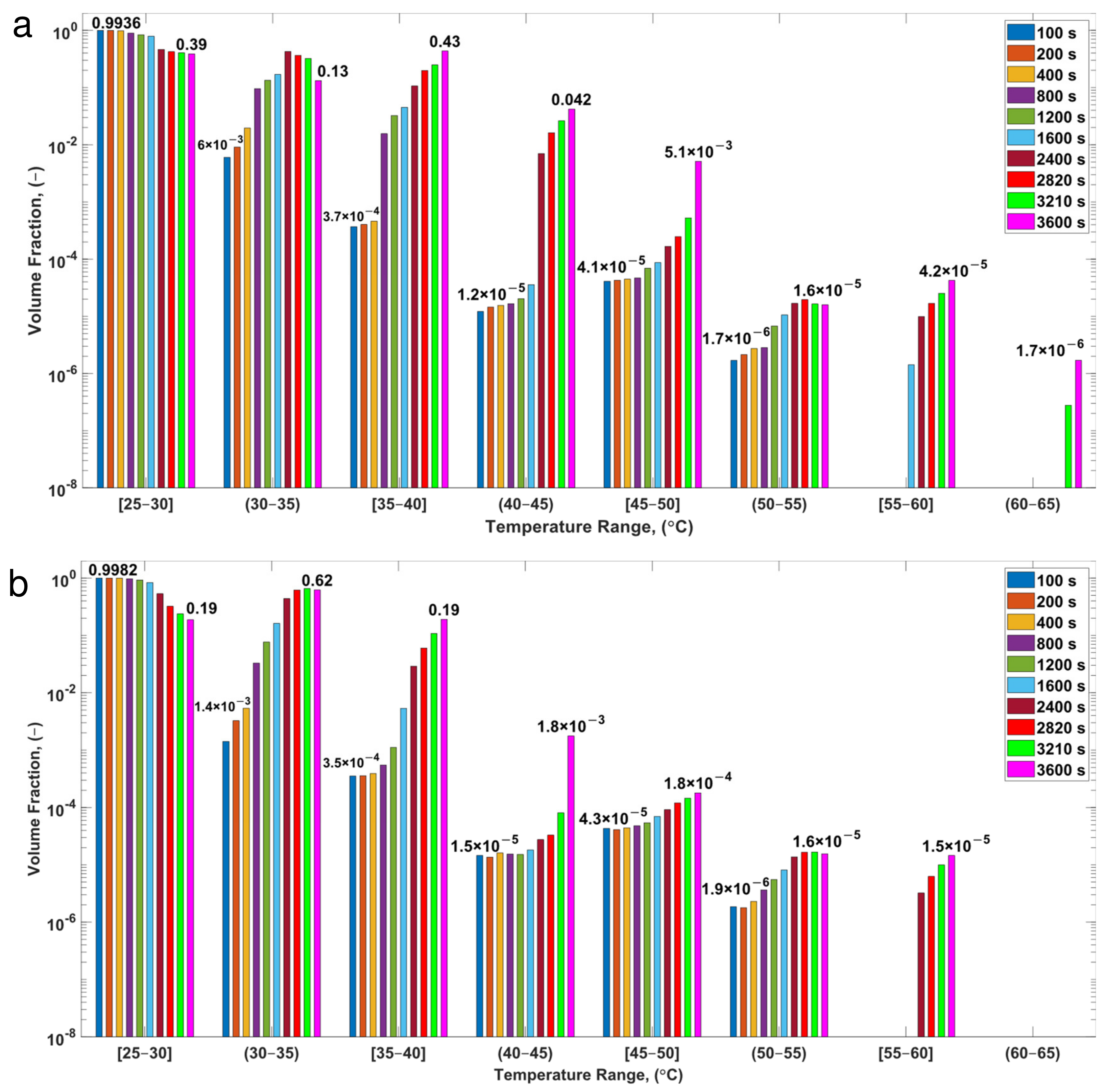
4.2.2. Volume Fraction Distribution

This section discusses volume fraction distribution histograms using the analogy of residence time distribution (RTD) in a non-ideal chemical reactor. In a perfect continuous stirred tank reactor (CSTR), the effluent concentration is identical to the concentration inside the reactor. Because of dead volumes (stagnant zones) in a realistic CSTR, certain particles remain for more prolonged periods than others. Similarly, owing to thermal stratification-induced mixing, only a portion of the pool participates in the heat removal process, while the remainder does not.
Figure 10 depicts the volume fraction distribution for a specific temperature range, from which the following conclusions may be drawn. After 3600 s, 31% of the pool water volume had a temperature increase of less than 5 °C, which is 2/3 of the volume-averaged, or well-mixed, pool temperature rise over this period. Secondly, much of the pool, or 34%, is between 30–35 °C. Similarly, at the end of the 3600 s, 30% of the water in the pool is between 35 and 40 °C, and 69% is between 30 and 45 °C. In the temperature range of 30–35 °C, a maximum volume fraction of 0.48 is found at 2820 s, falling to 0.41 after 3210 s. This decline results from the volume percentage of water in the higher temperature zones (35–40 °C) increasing with time. Additionally, water above 45 °C comprises less than 0.1% of the pool. This may be attributable to the fact that the higher temperature zones (>45 °C) are confined to SCRs with volumetric heat sources.
Significant overheating of just the top layers of the pool water is a characteristic signature of thermal stratification. Because the air in the containment vessel equilibrates with this layer of water, significant evaporation and pressure rise in the containment may thus occur as a result of thermal stratification.

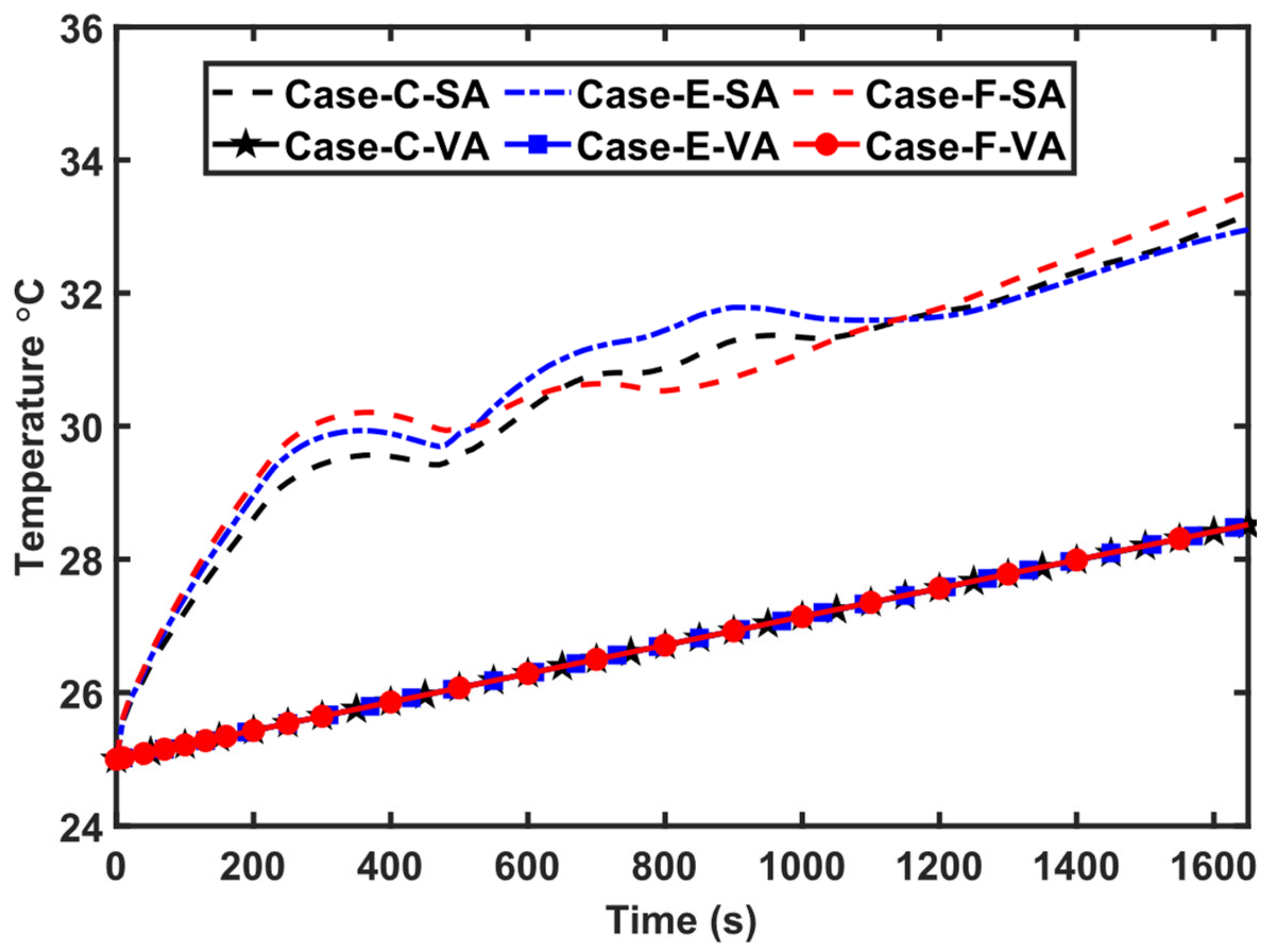
4.3. Parametric Influence

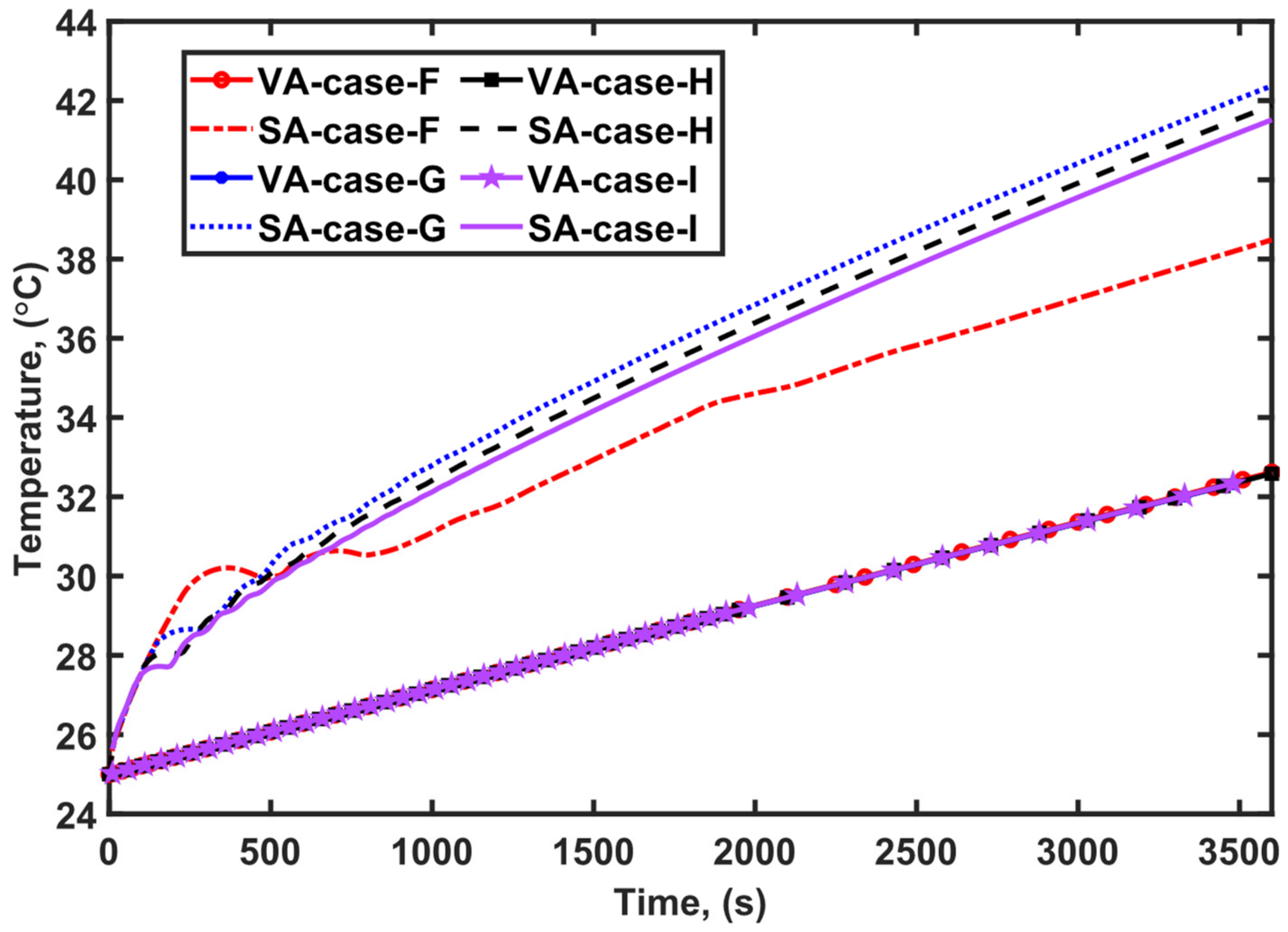
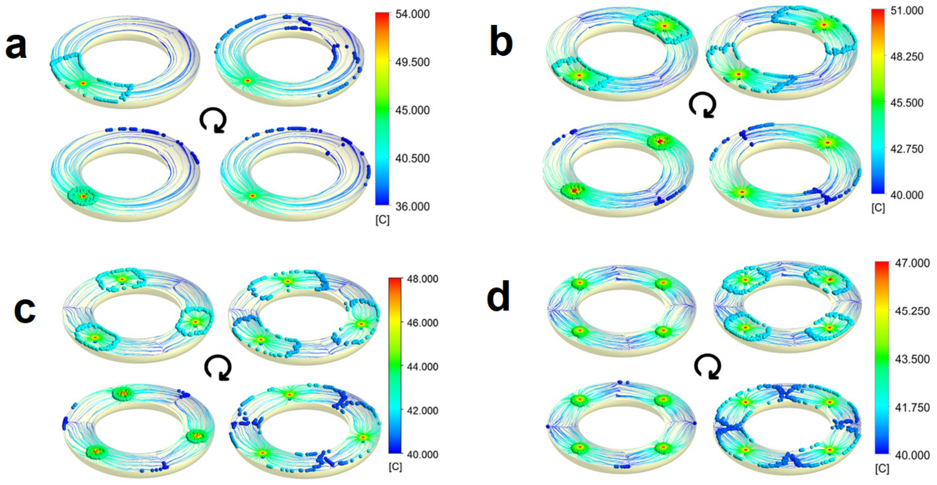
4.3.1. Effect of Number of Steam Injection Points (Heat Sources)

This part explores the influence of the multiple injection points on the condensing steam, which is modelled in the present study as multiple heat sources or steam condensing regions spread around the torus. In the case of multiple heat sources, they are assumed to be evenly spaced apart, and the total volumetric heat flux is conserved by dividing it among the number of sources. Consequently, two balancing processes co-occur: first, a drop in buoyant flux for a source, and second, a decrease in the per-capita volume of water available to dissipate heat before colliding with an incoming thermal front.
Figure 11 compares the surface temperature (averaged for the entire gas–liquid interface) evolution with time for the four cases, viz., F, G, H, and I, having one, two, three, and four steam injection points, respectively. It can be seen from Figure 11 that, typically, the surface temperature rises rapidly, plateaus for a brief period, starts decreasing, again plateaus, and starts increasing again. In case F, one can clearly see a few cycles of this behaviour before a pattern of linear increase occurs. In the other three cases with more injection points and thus smaller source strength, this cyclical pattern can still be seen, though with more rapidity as the number of sources increases. This pattern can be readily attributed to the tunnelling effect and the consequent pattern of convective transport of heat to the surface layer from the SCR. The initial rapid rise of the surface temperature occurs as the freshly heated water rises to the surface and spreads circumferentially. As it spreads, it also starts to lose heat by conduction to the lower layers. This eventually leads to the plateauing. This continues as the surface fronts collide, dive deeper, and circulate in the cooler waters to reach the SCR. Once the circulating water reaches the SCR, it can again pick up heat and appear at the surface hotter than before. This process continues with diminished strength due to the heating up of the top layers of the pool; after this, the temperature rise follows a linear path corresponding to the case where the water up to some depth (see the thermocline in Figure 4) reaches a fairly constant value.
The surface temperature rise pattern in cases G, H, and I needs to be seen in the above context. Close examination of the curves in Figure 11 shows that each case follows a similar pattern consistent with the above picture in two respects: decreasing source strength with increasing number of sources leading to more muted effect (i.e., smaller amplitude) of temperature oscillations, and shorter time of circulation with increasing number of sources as the distance of traverse lessens. It is also evident from Figure 11 that, with multiple heat sources, the surface temperature, after the initial tunnelling phase, decreases marginally with an increased number of heat sources. The surface temperatures at the end of 3600 s observed for the cases of one, two, three, and four heat sources (cases F, G, H and I) are 38.45, 42.35, 41.85, and 41.55 °C, respectively.
Figure 12a–d shows the streamlines emanating from the heat source at 3600 s, and the temperature difference between the hottest (above the heat source) and coldest (farthest location at the time of collision) points decreases with an increase in the number of sources. The maximum temperature declined from 51 °C to 47 °C as the number of sources increased, which is directly attributable to the reduction in the volumetric heat flow per source. The temperature difference ( Δ T s u r f ) decreased from 11 °C to 7 °C when the sources were increased from two to four as the buoyant plume’s temperature decreased to about 40 °C by the time of collision with an approaching front. Hence, this could be the reason for lower surface temperatures with heat sources increased from two to four. However, when it comes to a single source, though the maximum temperature on the surface is 54 °C as seen in Figure 12a, it has a longer traversing length until collision and, therefore, can dissipate more heat in the process, thereby reaching a substantially lower temperature of 36 °C. This could be the reason for the lower surface temperature for a single source compared to multiple heat sources.
Comparing the average temperatures with respect to elevation ranges (Figure 13), we see that, for a single-heat-source case, the stagnant zone not participating in the heat evacuation process is up to 75 mm elevation, whereas, for multiple heat sources, the stagnant zone is up to 100 mm. Further, when the volume fraction distributions are assessed at the end of 3600 s (Figure 14) for cases with multiple sources, about 50% of the pool volume is with a <5 °C increase in temperature, compared to 31% of the pool volume in the single-source case, indicating a steeper thermal stratification in case of multiple sources. About 34% of the pool is between 30 and 35 °C for a single heat source, whereas less than 5% is in the same range for multiple heat sources. Similarly, by the end of the 3600 s, 35% and 49% are in the temperature range of 35 to 45 °C for a single source and multiple sources, respectively.

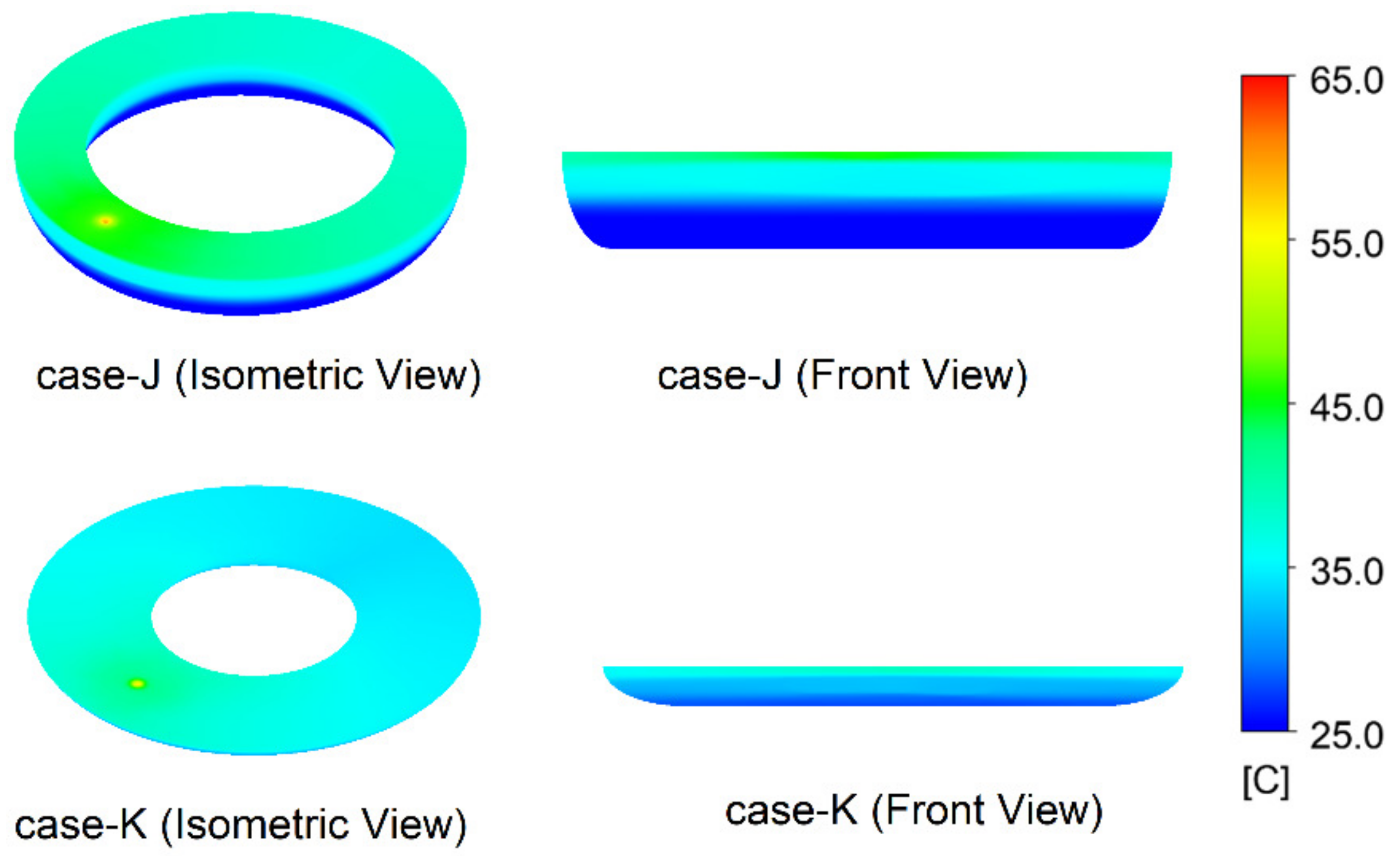
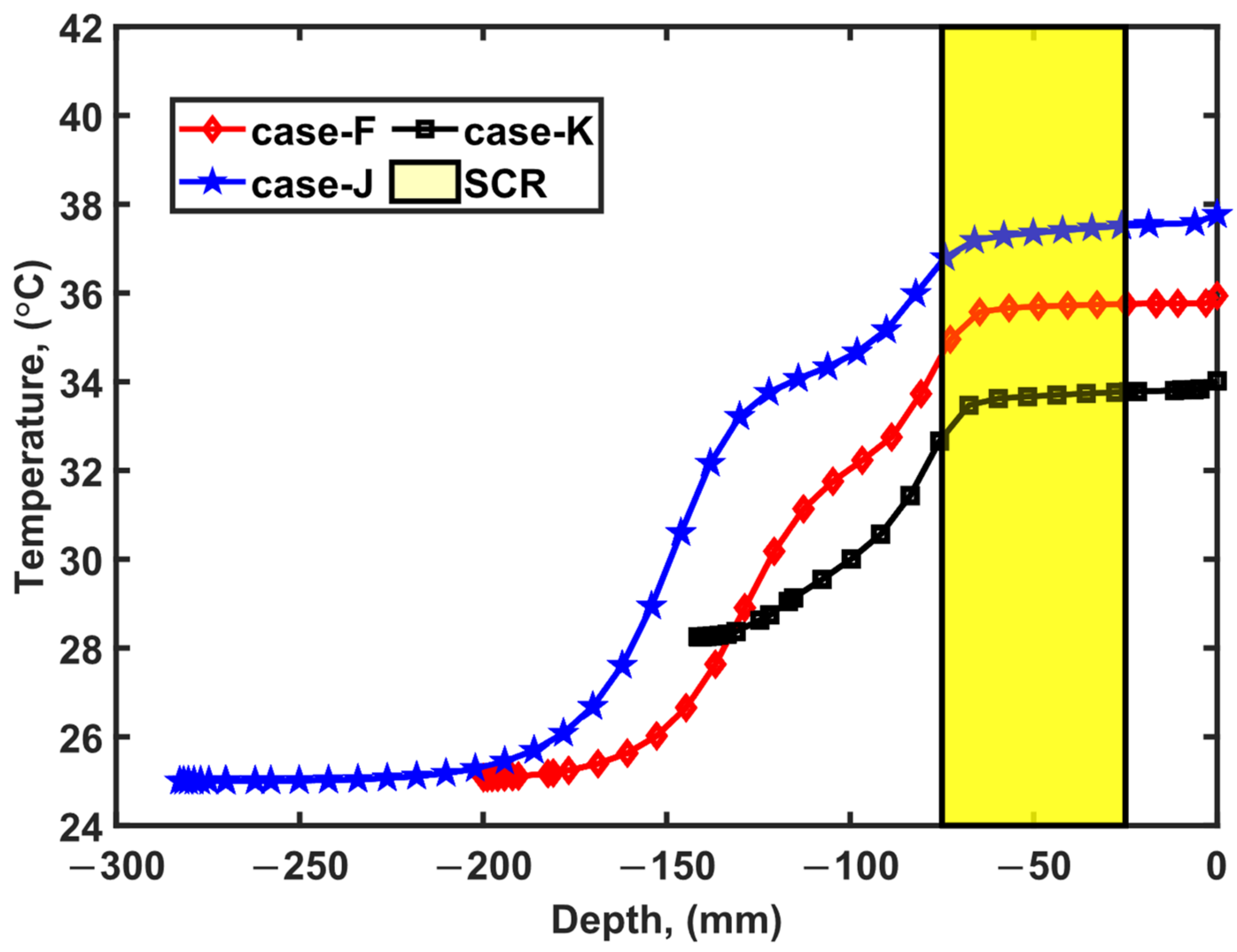
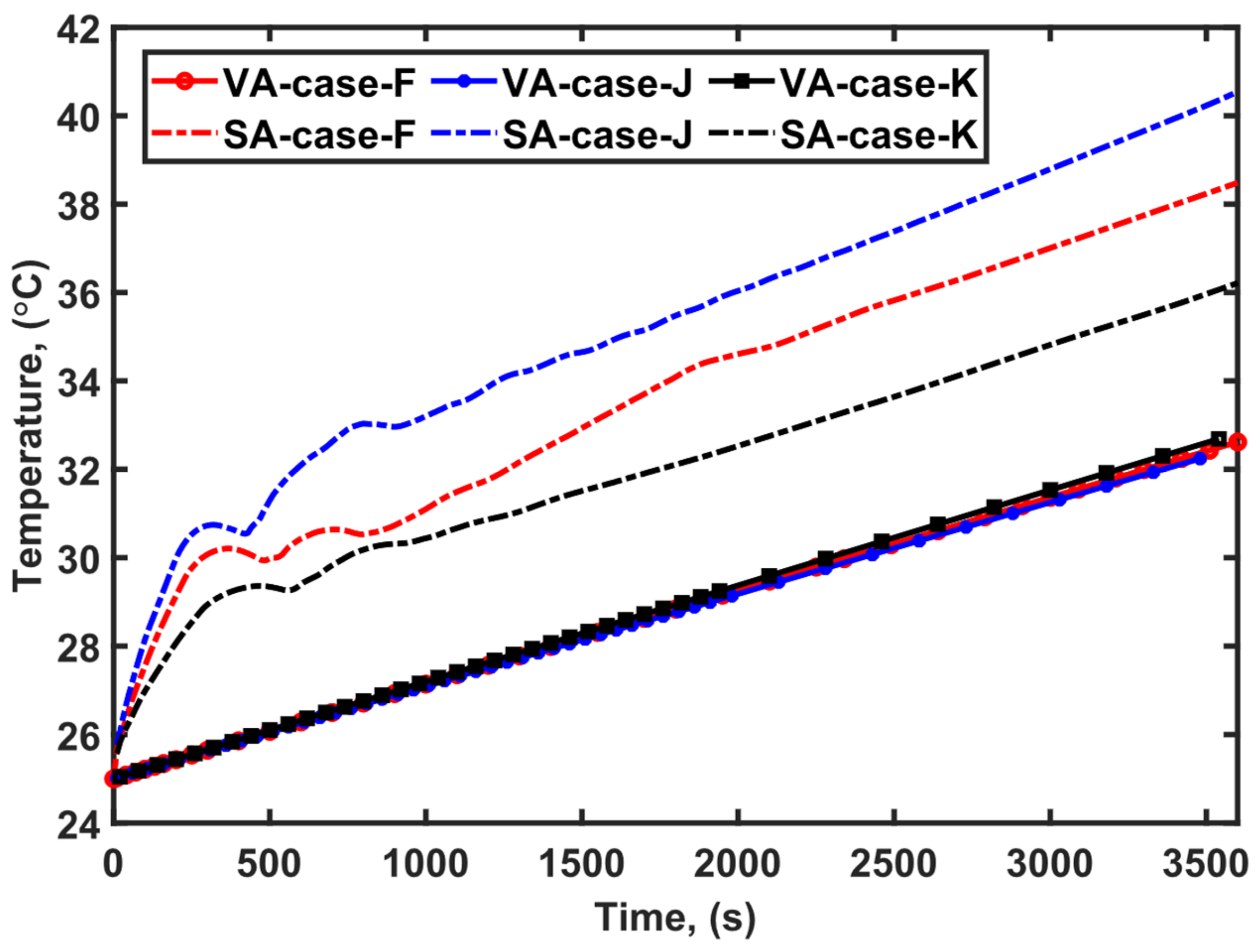
4.3.2. Effect of Aspect Ratio or Pool Cross-Section

The effect of aspect ratio is brought out in this section by varying the cross-sectional width to the depth of the pool for the same amount of water volume in the pool. The aspect ratio is the ratio of cross-sectional width to depth. For an aspect ratio of 0.5, the cross-sectional width is reduced, and the depth is increased to preserve volume resulting in a deeper and narrower pool. For an aspect ratio of 2.0, it is the depth that is reduced at the expense of width resulting in a shallower and wider pool. The dimensions for different cases are given in Table 4. Figure 15 displays the form of the geometry, as well as temperature contours for these scenarios; Figure 16 shows the thermocline for the three cases. It may be noted that, in all the three cases (F, J, and K), the same volumetric heat source and submergence depth are maintained along with other simulation parameters. Figure 15 shows that the quantity of water not participating in the heat evacuation process is more significant in the case of a deeper pool or lower aspect ratio (case J) than in the situation with a shallower pool (case K). It can be seen in Figure 15 and Figure 16 that case K’s lowest temperature is around 28 °C with a negligible dead zone, whereas case J’s temperature rise is almost stagnant between 175 and datum level depths. Thus, the effect of stratification is more pronounced in a deeper pool.
Figure 17 shows the time variation in the surface temperature for these three cases dealing with the effect of the aspect ratio of the pool. Consistent with the above observation of a stronger thermal stratification effect in a deeper pool, we find that the average surface temperature is substantially higher in case J than in case K. From the variation in the initial temperature associated with the thermocline formation, one can infer from Figure 17 that a stronger circulation is induced in the deeper pool leading to a faster rise in the surface temperature. However, since the dead pool volume is higher, a lesser fraction of the pool water participates in heat evacuation leading to substantially higher increases in surface temperature, and thus eventually to a greater increase in containment pressure.
The maximum average surface temperature for aspect ratios 0.5 and 2.0 is just above 40 °C and 36 °C, respectively. Although much of the pool is at less than 40 °C in both circumstances, as seen in Figure 18, it is crucial to note that 43% of the water is between 35–40 °C and 52% is between 25–35 °C in the deeper and narrower pool (lower aspect ratio) scenario, whereas 81% of the water in the higher-aspect-ratio case is between 25–35 °C. This implies that much of the pool contributes to the heat evacuation process for cases with a higher aspect ratio. It can also be noted from Figure 19 that the average temperatures for a given depth/height are lower by 4–5 °C for a high-aspect-ratio case (K) compared with one with a lower-aspect-ratio case (J).

5. Conclusions

In the present work, the buoyancy-induced circulation consequent to steam condensation in a reduced-scale, toroidal pool of water was studied using computational fluid dynamics (CFD) simulations with a view to understanding role of important design parameters of the suppression pool system. To this end, simulations of thermal stratification have been conducted using the effective heat source (EHS) approach for low steam flow rates, assuming the steam entirely condenses instantly in the proximity of the sparger. The EHS model has been applied by introducing a volumetric heat source equal to the latent heat of steam condensation for a given flow rate. The development of thermal stratification, its characteristics and the parametric influence of the pool shape, and the number of steam injection points have been studied numerically using CFD simulations. The results are discussed in terms of volume fraction and temperature distribution histograms using the analogy of residence time distribution (RTD) in a non-ideal chemical reactor. Additionally, the results have been interpreted in terms of the induced circulation pattern, establishment of a thermocline, and convective and diffusive dissipation of heat of condensation of steam. The following conclusions can be drawn from this study:
  • The tunnelling effect reported in the literature [34,36,37] encountered during the development of buoyancy-induced thermal stratification in a toroidal suppression pool has been delineated.
  • Due to the tunnelling effect, a persistent thermal stratification always develops, resulting in a higher surface average temperature than the bulk average temperature.
  • The surface temperature is shown to be significantly impacted significantly by the aspect ratio of the pool and moderately by the number of steam injection points.
  • For cases with multiple injections, about 50% of the pool volume is has a <5 °C increase in temperature, compared to 31% of the pool volume in a single-injection case, indicating a steeper thermal stratification in the case of multiple injections, reflected in a higher average surface temperature.
  • Observations based on the parametric influence of aspect ratio suggest that the baseline pool temperature rose by a maximum of 10 °C for 81% and 52% of the pool volume for aspect ratios of 2 and 0.5, respectively, demonstrating that a large portion of the pool participates in the heat evacuation process in cases with a larger aspect ratio.

Author Contributions

Conceptualization, S.B.K., S.M.A., and S.J.; methodology, S.B.K.; validation, S.B.K.; formal analysis, S.B.K. and S.J.; investigation, S.B.K.; resources, S.J.; data curation, S.B.K. and S.J.; writing—original draft preparation, S.B.K.; writing—review and editing, S.B.K., S.M.A., and S.J.; supervision, S.J. All authors have read and agreed to the published version of the manuscript.

Funding

This research received no external funding.

Conflicts of Interest

The authors declare no conflict of interest.

References

  1. Pellegrini, M.; Dolganov, K.; Herranz, L.E.; Bonneville, H.; Luxat, D.; Sonnenkalb, M.; Ishikawa, J.; Song, J.H.; Gauntt, R.O.; Fernandez Moguel, L.; et al. Benchmark Study of the Accident at the Fukushima Daiichi NPS: Best-Estimate Case Comparison. Nucl. Technol. 2016, 196, 198–210. [Google Scholar] [CrossRef]
  2. Mizokami, S.; Yamada, D.; Honda, T.; Yamauchi, D.; Yamanaka, Y. Unsolved Issues Related to Thermal-Hydraulics in the Suppression Chamber during Fukushima Daiichi Accident Progressions. J. Nucl. Sci. Technol. 2016, 53, 630–638. [Google Scholar] [CrossRef] [Green Version]
  3. Pellegrini, M.; Araneo, L.; Ninokata, H.; Ricotti, M.; Naitoh, M.; Achilli, A. Suppression Pool Testing at the SIET Laboratory: Experimental Investigation of Critical Phenomena Expected in the Fukushima Daiichi Suppression Chamber. J. Nucl. Sci. Technol. 2016, 53, 614–629. [Google Scholar] [CrossRef] [Green Version]
  4. Jo, B.; Erkan, N.; Takahashi, S.; Song, D.; Sagawa, W.; Okamoto, K. Thermal Stratification in a Scaled-down Suppression Pool of the Fukushima Daiichi Nuclear Power Plants. Nucl. Eng. Des. 2016, 305, 39–50. [Google Scholar] [CrossRef]
  5. Solom, M.; Vierow Kirkland, K. Experimental Investigation of BWR Suppression Pool Stratification during RCIC System Operation. Nucl. Eng. Des. 2016, 310, 564–569. [Google Scholar] [CrossRef]
  6. Cavaluzzi, J.; Andrs, D.; Vierow Kirkland, K. Two-Zone Stratified Wetwell Model Development and Implementation for RELAP-7. Ann. Nucl. Energy 2021, 164, 108592. [Google Scholar] [CrossRef]
  7. Li, H.; Villanueva, W.; Kudinov, P. Approach and Development of Effective Models for Simulation of Thermal Stratification and Mixing Induced by Steam Injection into a Large Pool of Water. Sci. Technol. Nucl. Install. 2014, 2014, 108782. [Google Scholar] [CrossRef] [Green Version]
  8. Gallego-marcos, I.; Villanueva, W.; Kudinov, P. Modelling of Pool Stratification and Mixing Induced by Steam Injection through Blowdown Pipes. Ann. Nucl. Energy 2018, 112, 624–639. [Google Scholar] [CrossRef]
  9. Villanueva, W.; Li, H.; Puustinen, M.; Kudinov, P. Generalization of Experimental Data on Amplitude and Frequency of Oscillations Induced by Steam Injection into a Subcooled Pool. Nucl. Eng. Des. 2015, 295, 155–161. [Google Scholar] [CrossRef]
  10. Zhang, Y.; Lu, D.; Wang, Z.; Fu, X.; Cao, Q.; Yang, Y.; Wu, G. Experimental Research on the Thermal Stratification Criteria and Heat Transfer Model for the Multi-Holes Steam Ejection in IRWST of AP1000 Plant. Appl. Therm. Eng. 2016, 107, 1046–1056. [Google Scholar] [CrossRef]
  11. Qu, X.; Revankar, S.T.; Tian, M. Numerical Investigation on Thermal Status of a Scaled-down Suppression Pool. Nucl. Eng. Des. 2018, 340, 183–192. [Google Scholar] [CrossRef]
  12. Gamble, R.E.; Nguyen, T.T.; Shiralkar, B.S.; Peterson, P.F.; Greif, R.; Tabata, H. Pressure Suppression Pool Mixing in Passive Advanced BWR Plants. Nucl. Eng. Des. 2001, 204, 321–336. [Google Scholar] [CrossRef]
  13. Kang, H.S.; Song, C.H. CFD Analysis for Thermal Mixing in a Subcooled Water Tank under a High Steam Mass Flux Discharge Condition. Nucl. Eng. Des. 2008, 238, 492–501. [Google Scholar] [CrossRef]
  14. Moon, Y.T.; Lee, H.D.; Park, G.C. CFD Simulation of Steam Jet-Induced Thermal Mixing in Subcooled Water Pool. Nucl. Eng. Des. 2009, 239, 2849–2863. [Google Scholar] [CrossRef]
  15. Song, C.H.; Kim, Y.S. Direct Contact Condensation of Steam Jet in a Pool. In Advances in Heat Transfer; Elsevier Inc.: Amsterdam, The Netherlands, 2011; Volume 43, pp. 227–288. ISBN 9780123815293. [Google Scholar]
  16. Wang, X.; Grishchenko, D.; Kudinov, P. Pre-Test Analysis for Definition of Steam Injection Tests through Multi-Hole Sparger in PANDA Facility. Nucl. Eng. Des. 2022, 386, 111573. [Google Scholar] [CrossRef]
  17. Song, D.; Erkan, N.; Jo, B.; Okamoto, K. Dimensional Analysis of Thermal Stratification in a Suppression Pool. Int. J. Multiph. Flow 2014, 66, 92–100. [Google Scholar] [CrossRef]
  18. Song, D.; Erkan, N.; Jo, B.; Okamoto, K. Relationship between Thermal Stratification and Flow Patterns in Steam-Quenching Suppression Pool. Int. J. Heat Fluid Flow 2015, 56, 209–217. [Google Scholar] [CrossRef]
  19. Gallego-Marcos, I.; Kudinov, P.; Villanueva, W.; Puustinen, M.; Räsänen, A.; Tielinen, K.; Kotro, E. Effective Momentum Induced by Steam Condensation in the Oscillatory Bubble Regime. Nucl. Eng. Des. 2019, 350, 259–274. [Google Scholar] [CrossRef]
  20. Liu, X.; Xie, X.; Meng, Z.; Zhang, N.; Sun, Z. Characteristics of Pool Thermal Stratification Induced by Steam Injected through a Vertical Blow down Pipe under Different Vessel Pressures. Appl. Therm. Eng. 2021, 195, 117169. [Google Scholar] [CrossRef]
  21. Cai, J.; Jo, B.; Erkan, N.; Okamoto, K. Effect of Non-Condensable Gas on Thermal Stratification and Flow Patterns in Suppression Pool. Nucl. Eng. Des. 2016, 300, 117–126. [Google Scholar] [CrossRef]
  22. Kumar, S.; Grover, R.B.; Vijayan, P.K.; Kannan, U. Numerical Investigation on the Effect of Shrouds around an Immersed Isolation Condenser on the Thermal Stratification in Large Pools. Ann. Nucl. Energy 2017, 110, 109–125. [Google Scholar] [CrossRef]
  23. De Walsche, C.; de Cachard, F. Experimental Investigation of Condensation and Mixing during Venting of a Steam/Non-Condensable Gas Mixture into a Pressure Suppression Pool. In IAEA Rep: INIS-CH--022; Paul Scherrer Institute Scientific: Villigen, Switzerland, 2000; Volume 4, pp. 53–61. [Google Scholar]
  24. Li, H.; Kudinov, P.; Villanueva, W. Modeling of Condensation, Stratification, and Mixing Phenomena in a Pool of Water; Technical Report number NKS-225; Nordisk Kernesikkerhedsforskning, Roskilde: Stockholm, Sweden, 2010. [Google Scholar]
  25. Patel, G.; Tanskanen, V.; Kyrki-Rajamäki, R. Numerical Modelling of Low-Reynolds Number Direct Contact Condensation in a Suppression Pool Test Facility. Ann. Nucl. Energy 2014, 71, 376–387. [Google Scholar] [CrossRef]
  26. Patel, G. Computational Fluid Dynamics Analysis of Steam Condensation in Nuclear Power. Ph.D. Thesis, Lappeenranta University of Technology, Lappeenranta, Finland, 4 April 2017. [Google Scholar]
  27. Choi, S.W. PUMA-PCCS Separate Effect Tests and RELAP5 Code Evaluation in PUMA. Ph.D. Thesis, Purdue University, West Lafayette, IN, USA, 2009. [Google Scholar]
  28. Jo, B.; Erkan, N.; Okamoto, K. Richardson Number Criteria for Direct-Contact-Condensation-Induced Thermal Stratification Using Visualization. Prog. Nucl. Energy 2020, 118, 103095. [Google Scholar] [CrossRef]
  29. Li, H.; Villanueva, W.; Puustinen, M.; Laine, J.; Kudinov, P. Thermal Stratification and Mixing in a Suppression Pool Induced by Direct Steam Injection. Ann. Nucl. Energy 2018, 111, 487–498. [Google Scholar] [CrossRef]
  30. Youn, D.H.; Ko, K.B.; Lee, Y.Y.; Kim, M.H.; Bae, Y.Y.; Park, J.K. The Direct Contact Condensation of Steam in a Pool at Low Mass Flux. J. Nucl. Sci. Technol. 2003, 40, 881–885. [Google Scholar] [CrossRef]
  31. Yang, Q.; Qiu, B.; Chen, W.; Zhang, D.; Chong, D.; Liu, J.; Yan, J. Experimental Study on the Influence of Buoyancy on Steam Bubble Condensation at Low Steam Mass Flux. Exp. Therm. Fluid Sci. 2021, 129, 110467. [Google Scholar] [CrossRef]
  32. Gallego-Marcos, I.; Kudinov, P.; Villanueva, W.; Kapulla, R.; Paranjape, S.; Paladino, D.; Laine, J.; Puustinen, M.; Räsänen, A.; Pyy, L.; et al. Pool Stratification and Mixing Induced by Steam Injection through Spargers: CFD Modelling of the PPOOLEX and PANDA Experiments. Nucl. Eng. Des. 2019, 347, 67–85. [Google Scholar] [CrossRef]
  33. Li, W.; Wang, J.; Sun, Z.; Zhou, Y.; Liu, J.; Meng, Z. Experimental Investigation on Thermal Stratification Induced by Steam Direct Contact Condensation with Non-Condensable Gas. Appl. Therm. Eng. 2019, 154, 628–636. [Google Scholar] [CrossRef]
  34. Filich, L. Modeling and Simulation of Thermal Stratification and Mixing Induced by Steam Injection through Spargers into Large Water Pool. Master’s Thesis, Royal Institute of Technology, Stockholm, Sweden, 2015. [Google Scholar]
  35. ANSYS, Inc. ANSYS Fluent User’s Guide; ANSYS, Inc.: Canonsburg, PA, USA, 2021. [Google Scholar]
  36. Hoshi, H.; Kawabe, R. Accident Sequence Analysis of Unit 1 to 3 Using MELCOR Code. In Proceedings of the Technical Workshop on the Accident of TEPCO’s Fukushima Dai-ichi NPS Handouts, 23 July 2012. [Google Scholar]
  37. Krepper, E.; Hicken, E.F.; Jaegers, H. Investigation of Natural Convection in Large Pools. Int. J. Heat Fluid Flow 2002, 23, 359–365. [Google Scholar] [CrossRef]
  38. Kota, S.B.; Ali, S.M.; Jayanti, S. Thermal Stratification Characteristics in a Reduced Scale Toroidal Suppression Pool. In Proceedings of the 8th International Conference on Advances in Energy Research (ICAER-2022), Mumbai, India, 7–9 July 2022; IIT Bombay: Mumbai, India, 2022; pp. 1–10. [Google Scholar]
Figure 1. A schematic of the torus and the steam condensation region where the volumetric heat flux is imposed.
Fluids 08 00020 g001
Figure 2. Various grids employed in the current study for mesh sensitivity, showing top views and sectional view of the mesh.
Fluids 08 00020 g002
Figure 3. (a) Space (grid) and time-step sensitivity study showing the temporal variation in temperature at three points at different heights, viz. 10 mm, 150 mm, and 200 mm along with the volume-averaged (VA) bulk temperature of the pool. (b) Non-dimensional temperature fluctuation in various grids relative to the finest grid (case D) at three points for different heights viz. 10 mm, 150 mm, and 200 mm.
Fluids 08 00020 g003
Figure 4. At 1600 s, a mesh sensitivity investigation shows thermocline variation at a position opposed to the steam condensation zone. Cases A, B, and C represent various meshes employed in the present work with decreasing coarseness. The shaded region shows the depth over which steam condensation takes place and heat is generated to drive the buoyancy current.
Fluids 08 00020 g004
Figure 5. Sensitivity study for the penetration length for the steam condensation region. The figure shows the temporal variation in surface average and bulk average temperatures. Cases C, E and F represent penetration lengths of 25 mm, 15 mm, and 10 mm, respectively.
Fluids 08 00020 g005
Figure 6. Validation of the present work by comparing temporal variation in temperature at location TT1 [4]. As seen in the above torus image, the graph’s markers reflect the positions of the points in the suppression pool relative to the SCR plane.
Fluids 08 00020 g006
Figure 7. Temporal variation in temperature at points located circumferentially: (a) on the surface of the pool, (b) at a depth of 50 mm from the surface.
Fluids 08 00020 g007
Figure 8. Streamlines in a torus emanating from the steam condensation zone, which is coloured with respect to temperature. The facets of the tunnelling phenomenon consist of (a) a heated plume rising from the region of the sparger, (b,c) expanding circumferentially, (d) sinking at the opposite ends of the sparger, and (ej) returning to the sparger at a lower height.
Fluids 08 00020 g008
Figure 9. Temporal variation in bulk average temperature with respect to the elevation ranges in the pool for the base case (Case F).
Fluids 08 00020 g009
Figure 10. Temporal variation in volume fractions on a logarithmic scale with respect to the temperature range in the suppression pool for the base case (Case F). It can be seen that, at a time of 3600 s, about 97% (or 0.31 + 0.34 + 0.33) of the pool volume is at a temperature lower than 40 °C.
Fluids 08 00020 g010
Figure 11. Temporal variation in average pool temperature and average surface temperature for one, two, three, and four heat sources (cases F, G, H, and I), respectively.
Fluids 08 00020 g011
Figure 12. Streamlines with markers emanating from volumetric heat sources at 3600 s for multiple heat sources: (a) case F, (b) case G, (c) case H and (d) case I. Each case has four sub-figures in a clockwise direction illustrating the makers travelling along the lines.
Fluids 08 00020 g012
Figure 13. Temporal variation in bulk average temperature with respect to the elevation ranges in the pool for number of heat sources: (a) two (Case G), (b) three (Case H), and (c) four (Case I), which are separated by 180°, 120°, and 90° respectively. Free surface temperature is area-averaged temperature.
Fluids 08 00020 g013
Figure 14. Temporal variation in volume fractions on a logarithmic scale with respect to the temperature range in the suppression pool for number of heat sources: (a) two (Case G), (b) three (Case H), and (c) four (Case I) which are separated by 180°, 120°, and 90° respectively.
Fluids 08 00020 g014
Figure 15. Temperature variation by the end of 3600 s for cases with an aspect ratio of 0.5 (Case J) and 2.0 (Case K).
Fluids 08 00020 g015
Figure 16. Thermocline at diametrically opposed ends of the SCR illustrating the influence of aspect ratio.
Fluids 08 00020 g016
Figure 17. Temporal variation in pool average temperature and surface average temperature for various aspect ratios.
Fluids 08 00020 g017
Figure 18. Temporal variation in volume fractions on a logarithmic scale with respect to the temperature range in the suppression pool for aspect ratios of (a) 0.5 (Case J) and (b) 2.0 (Case K).
Fluids 08 00020 g018
Figure 19. Temporal variation in bulk average temperature with respect to the elevation ranges in the pool for aspect ratios of (a) 0.5 (Case J) and (b) 2.0 (Case K); free surface temperature is area-averaged temperature.
Fluids 08 00020 g019
Table 1. Simulation matrix employed in the current study.
CaseRemarks and Simulation Inputs
AMesh 1; Penetration length = 25 mm
BMesh 2; Penetration length = 25 mm
CMesh 3; Penetration length = 25 mm
DMesh 3; Time step sensitivity; Penetration length = 25 mm
EPenetration length = 15 mm; Penetration length sensitivity.
VHF = X = 16.7 MW/m3; A = 1.0
FPenetration length = 10 mm; Penetration length sensitivity.
Base Case; VHF = X = 42.2 MW/m3; A = 1.0
Parametric Influence (No. of heat sources)
G2-heat sources
H3-heat sources
I4-heat sources
Parametric Influence (Aspect Ratio)
J A J = 0.5 A F
K A K = 2.0 A F
Table 2. Properties of water employed in the simulation.
PropertyValue
ρ , [ kg / m 3 ] 997.1
C p , [ J / ( k g . K ) ] 4182
k , [ W / ( m . K ) ] 0.6
μ , [ k g / ( m . s ) ] 0.001003
β , [ K 1 ] 0.0002594
Table 3. Comparison of experimental and simulated temperature increase rates at different locations.
Point Height, (mm) d T d t | e x p ,   ( ° C / s ) [4] d T d t | s i m ,   ( ° C / s )
1500.00220.0026
1000.00210.0022
105.2 × 10−45.5 × 10−5
Table 4. Dimensions of the torus for aspect ratios of 1 (case F), 0.5 (case J), and 2.0 (case K).
Aspect   Ratio ,   ( a / d )10.52
Volume (mm3)1.89 × 1081.89 × 1081.89 × 108
a ,   m m 200.00141.42282.84
d ,   m m 200.00282.84141.42
Disclaimer/Publisher’s Note: The statements, opinions and data contained in all publications are solely those of the individual author(s) and contributor(s) and not of MDPI and/or the editor(s). MDPI and/or the editor(s) disclaim responsibility for any injury to people or property resulting from any ideas, methods, instructions or products referred to in the content.

