Article

Modification of Poiseuille Flow to a Pulsating Flow Using a Periodically Expanding-Contracting Balloon

by
Iosif Moulinos
,
Christos Manopoulos
* and
Sokrates Tsangaris
Biofluid Mechanics & Biomedical Engineering Laboratory, School of Mechanical Engineering, National Technical University of Athens, 15780 Athens, Greece
*
Author to whom correspondence should be addressed.
Fluids 2023, 8(4), 129; https://doi.org/10.3390/fluids8040129
Submission received: 19 February 2023 / Revised: 1 April 2023 / Accepted: 7 April 2023 / Published: 12 April 2023
(This article belongs to the Section Mathematical and Computational Fluid Mechanics)

Abstract

:
Balloon pumps are employed to assist cardiac function in cases of acute myocardial infarction, ventricular arrhythmias, cardiogenic shock, unstable angina, refractory ventricular failure, or cardiac surgery. Counterpulsation, through increasing the diastolic pressure and reducing the systolic pressure, increases coronary perfusion and assists the heart to pump more blood at each contraction. An expanding-contracting balloon, modifying the Poiseuille flow in a straight circular duct, is examined in this study. The balloon is spheroid-shaped, with the length of its minor axis, which is perpendicular to the flow direction, changing in time following a sinusoidal law. The inlet flow volume rate is steady while the rate that the fluid volume leaves the duct varies in time due to the presence of the balloon. For a pulsation frequency of 60 pulses/min, the pressure difference across the pulsating balloon exhibits significant phase lagging behind the outflow volume waveform. The outlet pressure depends on the balloon radius oscillation amplitude and is computed for a range of such. The flow field around the spheroid, periodically expanding-contracting balloon in the steady flow stream is presented, in which the exact pattern of the gradual downstream intensification of the flow pulsation alongside the spheroid body is also identified.

1. Introduction

Blood flow in large arteries is pulsatile and laminar, described by a Fourier series whose zeroth harmonic is a steady Poiseuille flow, and its fundamental frequency is equal to the cardiac rhythm [1]. Womersley developed a method for calculating velocity, rate of flow, and viscous drag in arteries when the pressure gradient is known, which is commonly referred to as the “Womersley problem” [2].
Tsangaris and Stergiopulos addressed the inverse Womersley problem, which involves determining the time-varying flow field given the evolution of flow rate through a circular pipe over time [3]. They derived an equation expressing the developed flow velocity profile as a function of the time derivative of the flow rate and integrated it using finite differences. A first-order approximation was used for time derivatives, and a second-order central scheme was used for spatial derivatives.
The expanding-contracting balloon is used to contribute to the heart-driven pulsatile flow in the form of the intra-aortic balloon pump (IABP). Treatment with IABP is found to have a positive impact if received by patients facing situations such as unstable angina, acute myocardial infarction, ventricular arrhythmias, acute ischaemic mitral regurgitation, post infarct ventricular septal rupture, and percutaneous coronary intervention (PCI) [4]. Introduced by Moulopoulos et al., the IABP increases the diastolic blood flow in the arteries and lowers the end-diastolic arterial pressure, thus resulting in the amelioration of coronary blood circulation and decreased myocardial work, without taking blood out of the body [5].
In vitro experiments and clinical studies of the role of arterial stiffness in IABP therapy were presented by [6,7]. The authors found that augmentation of the arterial stiffness leads to a reduction of the systolic and the end-diastolic aortic pressure. Arterial stiffness is found to be more important than arterial pressure for the effectiveness of the IABP and is a potential additional parameter for deciding the use of IABP treatment. Applanation tonometry is proposed for compliance measurements and stiffness gain via pharmacological interventions. Using an in vitro bench, the increase of cardiac output under IABP treatment was examined by Xie et al. [8]. The placement of an aortic stent at the upstream end of the balloon gives augmented product of heart rate and stroke volume.
A rigid duct model for the thoracic aorta with cylindrical shaped IABP is examined by Bruti [9]. Pressure boundary conditions are imposed at both ends of the vessel, which are obtained by a zero-dimensional model of the arterial system. Computation of the flow field around the IABP during pulsed cardiopulmonary bypass (CPB) by Graminga et al. [10] showed increased perfusion during balloon inflation through the innominate, the left carotid, and the left subclavian arteries. It also recorded the transition from a rotational flow to an untwisted one in comparison with the case of non-pulsatile CPB. Different sizes and positions of the IABP were studied by Caruso et al. [11]. They found that flow volume through renal, mesenteric, and iliac arteries increases by decreasing the maximum balloon volume and the distance of the balloon from the left subclavian artery. The IABP therapy weaning process is calculated by Caruso et al. [12].
Using their zero-dimensional framework for the simulation of the cardiovascular system and mechanical circulatory and ventilation support [13], De Lazzari et al. verified the measured flow patterns present in the case of hemodynamic flow with an IABP for varying timing ratios [14]. The blood flow through the aorta in the presence of IABP or/and extracorporeal membrane oxygenation (ECMO) was studied by Gu et al. [15,16] using a finite element model.
In the present work, an expanding-contracting balloon modulates the steady incoming flow of a circular cross-section pipe. A numerical simulation of Poiseuille flow influenced by a spheroid shaped balloon expanding and contracting in the straight vessel is conducted using the curvilinear immersed boundary method. The Womersley number of the flow refers to 60 pulses per minute and the Reynolds number is a value corresponding to mean blood flow through the human thoracic aorta during a cardiac cycle. The output pressure wave of the configuration is presented and the correlation with the balloon volume change rate is discussed. The presentation of the time-evolving velocity and pressure fields around the prolate spheroid-shaped, sinusoidally pulsating balloon is an additional contribution of this research, clarifying the flow details of balloon pumping in this setting.

2. Materials and Methods

2.1. Governing Equations
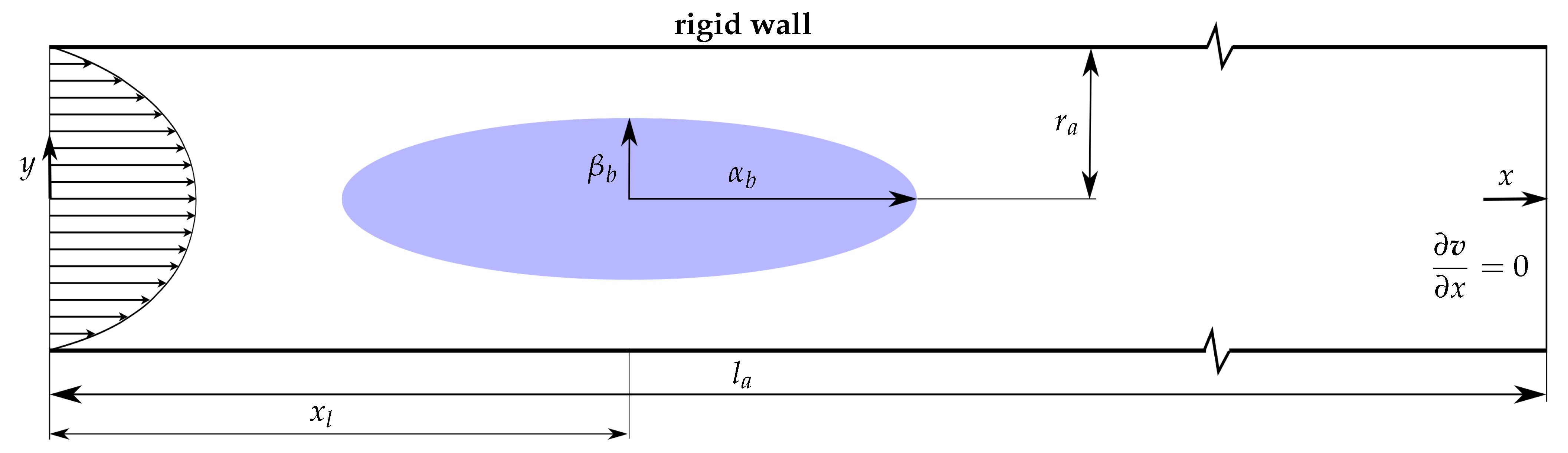
Blood perfusion in large arteries can be considered Newtonian [17] and with negligible compressibility [18] for the range of human hematocrit values. Under these assumptions, the mass conservation is expressed as
· v = 0 ,
and the conservation of momentum is expressed as
v t + · ( v v ) = 1 ρ p + ν 2 v ,
in which  v ( x , t )  is the fluid velocity,  x  is the position vector, t is time,  p ( x , t )  is the pressure field,  ρ  is the fluid density, and  ν  is the kinematic viscosity of the fluid.

2.2. Vessel Model

A schematic of the setting is shown in Figure 1. The vessel which contains the balloon is modeled as a straight tube of circular cross-section. The radius of the pipe is  r a  and its length is  l a .
The balloon shape is that of a prolate ellipsoid of revolution. The spheroid major axis identifies with the pipe axis of symmetry and its middle is at the longitudinal position  x l . The balloon surface in Cartesian coordinates follows the equation
( x x l ) 2 α b 2 + y 2 β b 2 ( t ) + z 2 γ b 2 ( t ) = 1 , | x x l | a b , β b ( t ) < r α , γ b ( t ) < r α ,
where  α b > β b = γ b  are the corresponding semi axes. The major semi axis length is steady in time whereas the median and minor semi axis vary in time following a cosine law,
β b ( t ) = γ b ( t ) = r b 0 A b c o s 2 π T t ,
where T is the period of the oscillation. Consequently, the balloon volume evolves in time as
V ( t ) = 4 3 π · α b · β b ( t ) · γ b ( t ) = 4 3 π · α b · r b 0 A b c o s 2 π T t 2 .
Hence, the fluid volume through the outlet, i.e., the pulsating flow volume rate is
Q o u t ( t ) = Q i n ( t ) + d V ( t ) d t = Q i n ( t ) + 8 3 · α b · A b π 2 T 2 · r b 0 · s i n 2 π T t A b · s i n 4 π T t .
The geometric values of the setting are presented in Table 1. The vessel radius is determined as the average value of the aorta radius at the locations corresponding to the aortic arch and the renal arteries, respectively, as reported in the work of Caruso et al. [11].
The inlet and outlet flow volume rate curves are depicted in Figure 2.
The fluid properties for the simulation are as in Table 2.
For period  T = 1  s, the non-dimensional frequency parameter (Womersley number) of the pulsating flow is
α = r α ω ν = 11.936 ,
where  ω = 2 π T  is the angular frequency of the balloon oscillation.

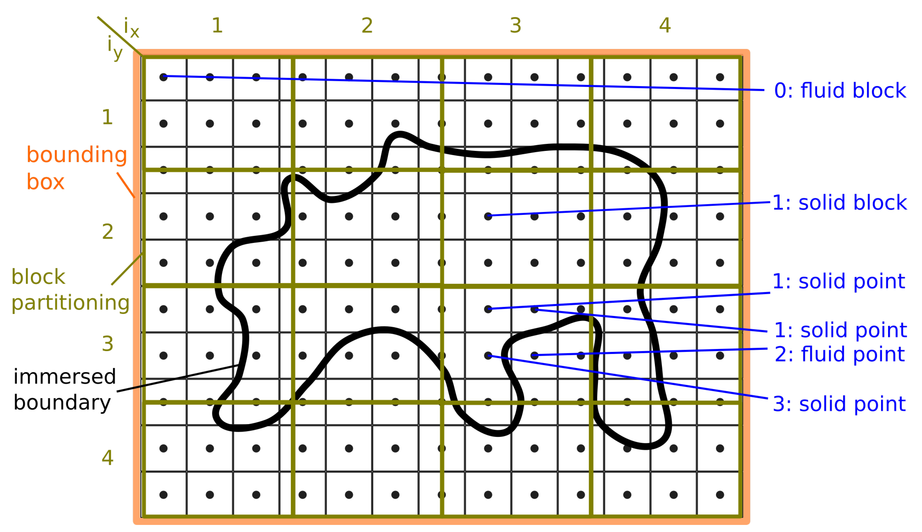
2.3. Numerical Method

The Navier–Stokes equations (Equations (1) and (2)) are handled via the curvilinear immersed boundary method [19] implemented in the Virtual Flow Simulator software [20]. The decoupling of the solution mesh from the body motion, which characterizes the immersed boundary method, ceases the need for mesh regeneration at each time step. Moreover, the curvilinear variant enables the exact imposition of the boundary conditions on the pipe surface. Application of the method for flow fields driven by deformable bodies, where fluid computational volume is not preserved in time, has provided satisfying results [21]. For the classification of the underlying mesh nodes as fluid, solid, and immersed boundary nodes, firstly a bounding box around the immersed surface is introduced. Points at the exterior of the box are marked as fluid. For points at the interior, uniform partitioning in blocks and implementation of the ray-tracing algorithm are performed. From each block or point of interest, a beam is emitted. In case the number of intersection points of the beam with the immersed boundary is congruent to 2 modulo 2, the beam source is labeled fluid, otherwise it is labeled solid (Figure 3) [22]. Finally, nodes with corresponding cells sharing a face with a solid cell are marked as immersed boundary nodes.
The immersed boundary surface is tessellated by triangles. Decision of the intersection of a ray with the immersed boundary is made by implementing the Möller–Trumbore algorithm [23]. Increased accuracy is required for the epsilon constant, used to decide whether the ray is parallel to the triangle in order to determine the relative position of a node and the immersed balloon  ϵ = 10 15 .
To comply with the solution framework, the conservation laws are converted on the basis of a curvilinear coordinate system  ξ = { ξ 1 , ξ 2 , ξ 3 } . The transformation is achieved by leveraging the curvilinear form of the derivative operators involved in Equations (1) and (2). By introducing the contravariant base,
g 1 = ξ 1 = ξ 1 x , ξ 1 y , ξ 1 z = ( ξ x 1 , ξ y 1 , ξ z 1 ) g 2 = ξ 2 = ξ 2 x , ξ 2 y , ξ 2 z = ( ξ x 2 , ξ y 2 , ξ z 2 ) g 3 = ξ 3 = ξ 3 x , ξ 3 y , ξ 3 z = ( ξ x 3 , ξ y 3 , ξ z 3 ) ,
for a scalar field  ϕ  and a vector field  Y  holds [24]
· Y = 1 J ξ j ( J g j · Y )
ϕ = g j ϕ ξ j = 1 J ξ j ( J g j ϕ )
2 ϕ = 1 J ξ j J g j · g k ϕ ξ k .
Hence, the governing equations take the form
1 J ξ j ( J U j ) = 0
J U k t + ξ x i k ξ j ( J U j u i ) = ξ x i k ξ j J ξ x i j p ρ + 1 ν ξ x i k ξ j J g j m u i ξ m ,
where
J = ( x 1 , x 2 , x 3 ) ( ξ 1 , ξ 2 , ξ 3 )
is the Jacobian determinant of the transformation from the Cartesian to the curvilinear coordinate system. The symbols  U k  are for the contravariant velocity components, and the symbols  u i  are for the Cartesian ones. The quantities
g j m = g j · g m = ξ j x 1 , ξ j x 2 , ξ j x 3 · ξ m x 1 , ξ m x 2 , ξ m x 3
are the elements of the metric tensor.
Equations (12) and (13) are solved for fluid nodes. At an immersed boundary node P, the flow field is computed by linear interpolation between two known velocity values along the normal to the immersed surface, passing through P. The first sample is the velocity of the immersed boundary and the second is the velocity of the intersection point of the closest fluid nodes triangle (Figure 4).
Flow equations are discretized via finite differences [25] and the Crank–Nicolson formulation is applied for time marching [26]. For the coupling of the momentum and continuity equations, the projection method of Chorin is employed [27]. The time step is constrained by the demand that a solid node of the underlying mesh cannot convert to a fluid node at the successive time step. Every solid node that is about to become a fluid one should necessarily convert firstly to an immersed boundary node in an intermediate step, in order to acquire valid flow variable values. Hence, the time step is bounded as
Δ t min i 1 , 2 , 3 Δ ξ i ( x ) U i ( x ) , x { solid points converting to fluid } .
The discrete momentum equations are handled by means of a Newton-based nonlinear iterative solver that uses a trust region [28]. The resulting linear systems are solved by the GMRES method [29], with the (block) Jacobi preconditioner. The discretized Poisson equation that arises for pressure is solved with the GMRES method, using the algebraic multigrid method as a preconditioner [30].

2.4. Boundary Conditions

By employing cylindrical coordinates  ( x , r , θ )  for the axial, the radial, and the tangent direction, respectively, the velocity is expressed as  ( u , U r , U θ ) , where  U r  is the radial velocity component and  U θ  is the peripheral velocity component.
On the inner boundary, namely on the surface of the balloon, fixed boundary conditions are imposed;
u x , r , θ , t ( x x l ) 2 α b 2 + r 2 β b 2 ( t ) = 1 , | x x l | a b = 0 U r x , r , θ , t ( x x l ) 2 α b 2 + r 2 β b 2 ( t ) = 1 , | x x l | a b = r ( x , t ) t = a b 2 ( x x l ) 2 · 2 π A b α b T s i n 2 π T t U θ x , r , θ , t ( x x l ) 2 α b 2 + r 2 β b 2 ( t ) = 1 , | x x l | a b = 0 .
On the outer boundary of the computational domain, mixed boundary conditions are imposed. At the inlet, only the axial velocity is non-zero with a parabolic profile,
u ( x = 0 , r , θ , t ) = Q i n π r a 2 2 1 y 2 + z 2 r a 2 U r ( x = 0 , r , θ , t ) = 0 U θ ( x = 0 , r , θ , t ) = 0 .
At the vessel wall, no slip condition is set,
u ( x , r = r a , θ , t ) = 0 U r ( x , r = r a , θ , t ) = 0 U θ ( x , r = r a , θ , t ) = 0 .
At the downstream end of the tube, zero longitudinal derivative of the velocity is demanded
u x ( x = l α , r , θ , t ) = 0 U r x ( x = l α , r , θ , t ) = 0 U θ x ( x = l α , r , θ , t ) = 0 .
Taking advantage of the symmetry of the geometry and the flow field, and taking into consideration the structure of the solution algorithm, a quarter cylinder geometry is examined. Symmetry boundary conditions are imposed at the two longitudinal section planes, i.e., steady meridional velocity with respect to the tangent direction and zero peripheral velocity,
u θ ( x , r , θ = 0 , t ) = u θ ( x , r , θ = π 2 , t ) = 0 U r θ ( x , r , θ = 0 , t ) = U r θ ( x , r , θ = π 2 , t ) = 0 U θ ( x , r , θ = 0 , t ) = U θ ( x , r , θ = π 2 , t ) = 0 .

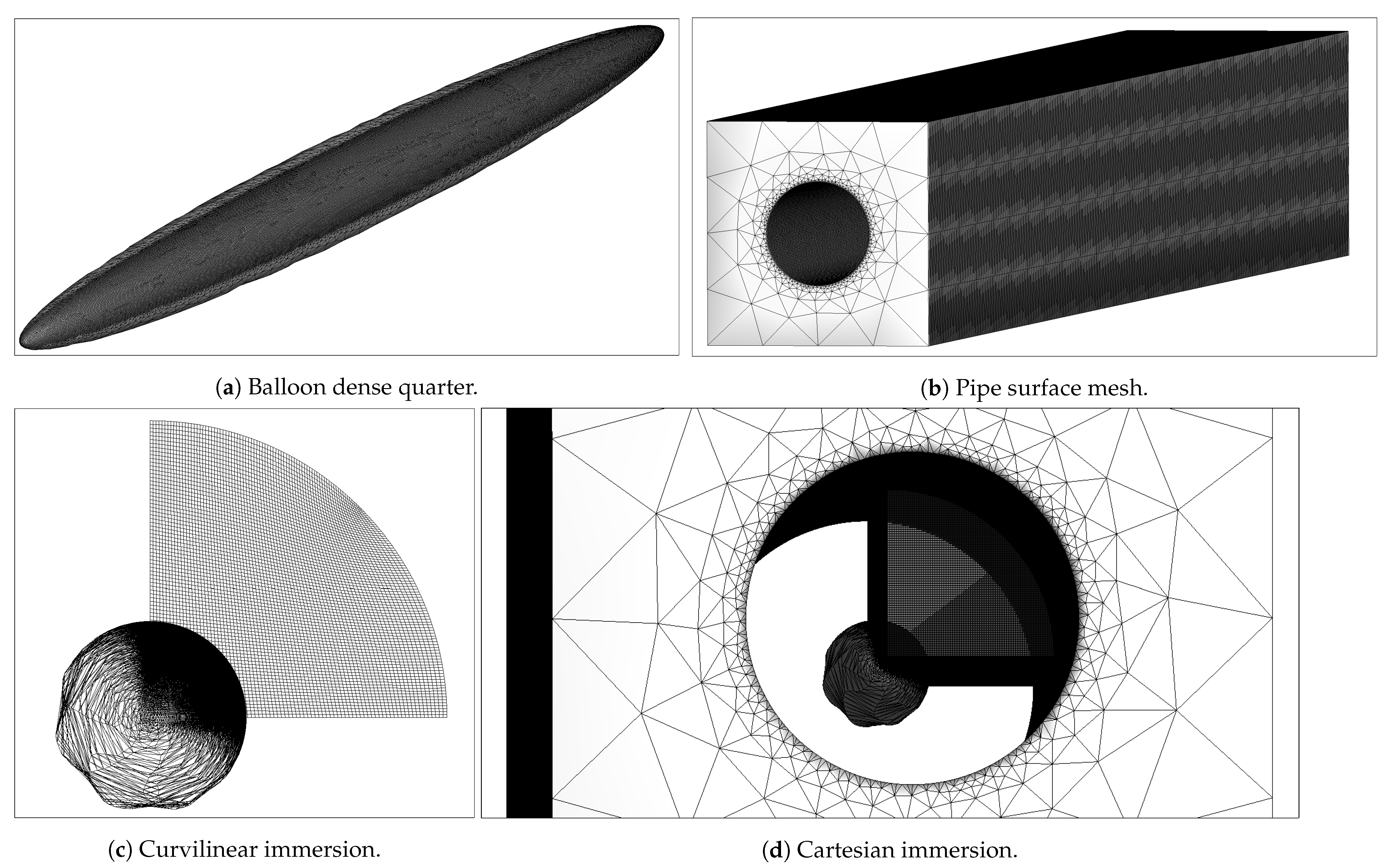
2.5. Space and Time Domain Discretization
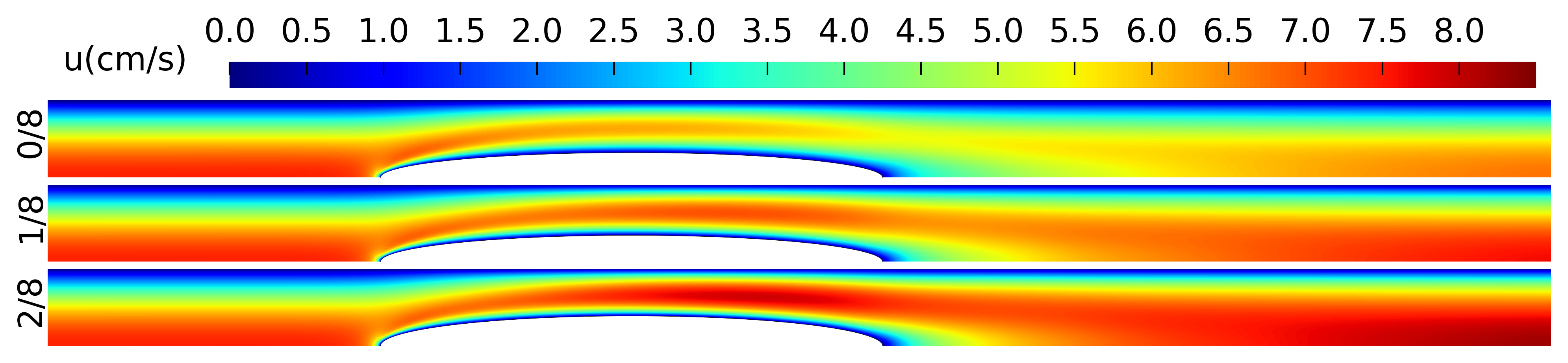
Flow Equations (12) and (13) are solved on both curvilinear and Cartesian underlying meshes. In the first case, the boundary conditions at the curved surface of the cylinder are set exactly, while in the second, they are imposed by interpolating between the closest triangle of fluid nodes and the neighboring immersed boundary nodes. To certify independence of the solution from the computational grid, meshes of increasing density are used.
The concluding, finest curvilinear, consists of  80 × 80  nodes in a parallel plane to the cylinder vessel base, while the Cartesian consists of  97 × 97  nodes. Both the curvilinear and the Cartesian grids in the flow direction in the interval  3.6 x ( c m ) 10.6  consist of cells with  δ x = 0.02  cm. In the region  0 x ( c m ) 3.6 δ x  follows a geometric sequence starting from the value  δ x = 0.08  cm and concluding to  δ x = 0.02  cm. Finally, downstream of the balloon, within the region  10.6 x ( c m ) 18 δ x  increases, following a geometric sequence with first term  δ x = 0.02  cm and last  δ x = 0.12  cm. The total number of nodes in the axial direction is 558. For a Cartesian mesh consisting of  66 × 66 × 410  nodes in the transverse plane and the flow direction, respectively, the maximum difference in outlet pressure comparing to the finest Cartesian mesh is  0.7 %. The respective difference in outflow velocity at the center of the pipe is  0.019  cm/s.
The expanding-contracting balloon is triangulated by a  31,206  nodes and  62,408  elements grid and the pipe discretization consists of  72,756  nodes and  145,508  elements as shown in Figure 5.
Time integration is performed with steps of magnitude  δ t = 0.00002  s.

3. Results

The resulting velocity vectors on a plane defined by the pipe main axis and a generator axis of the cylinder are depicted in Figure 6. Axial velocity contours are given in Figure 7.
Radial velocity contours are given in Figure 8 and pressure distribution contours are given in Figure 9. More detailed depiction of the velocity field is given in Appendix A.
The evolution of the outlet pressure,  p o u t , in time is given in Figure 10.
The outlet longitudinal velocity profiles are given in Figure 11.
The difference between the outlet and inlet axial velocity profiles is given in Figure 12.

4. Discussion

The flow around an expanding-contracting balloon is studied, where the pulsating closed surface membrane is spindle-shaped, with an oscillating equatorial radius magnitude. The Womersley number is  11.936 , which corresponds to the periodic cardiac flow in the human aorta. The mean Reynolds numbers used in the present paper are 182, 730, and 1515. The lower value corresponds to inlet flow  Q i n = 0.01  L/s, while the higher value corresponds to inlet volume  Q i n = 0.0833  L/s, which is the average resting cardiac output for both trained and sedentary individuals [12,31,32]. The flow fields, computed via (a) structured curvilinear meshes, body fitted at the vessel geometry and (b) structured Cartesian meshes, considering the vessel an immersed boundary, are in good agreement.
The inlet parabolic profile at the pipe cross section transitions to a toroid profile around the pulsating balloon’s lengthwise center, with a cross section resembling that of the oscillating flow over the cross section of an annular pipe [33]. Downstream of the balloon, the radial velocity component tends to restore the maximization of the longitudinal velocity profile on the pipe axis. The maximum, over the cross section, vectors are of a larger magnitude near the inlet and are shorter at the balloon region, as expected by mass conservation.
As shown in Figure 7, at the part of the period where the balloon volume change rate increases, the outflow volume rate increases. The maximizer of Equation (6) is
arg max t [ 0 , T ) Q o u t ( t ) = T 2 π arccos r b 0 A b r b 0 2 A b 2 + 8 4 ,
for which a dark red region emerges near the outflow. For the rest of the period, where the balloon volume change rate decreases, the outflow volume rate follows the same trend. For  t = 3 T / 4 , the longitudinal velocity near the outlet is minimal. The low velocity region near the outer wall has a smaller thickness in the region  4 x ( c m ) 10 , where the balloon is placed, due to the viscous effects in the duct between the wall and the moving surface of the balloon.
At the position where the incoming fluid velocity profile attacks the balloon, a high radial velocity region is created, as the streamlines curve in order to adjust to the geometry (Figure 8). The length of the high radial velocity component region achieves grosso modo higher values during inflation than during deflation. The radial velocity field exhibits the maximum intensity for  t = T / 4 , triggered by the maximization of the balloon surface’s oscillation velocity. The most extended intensely negative region emerges for  t = 3 T / 8  as the result of large balloon oscillation displacement and high flow volume rate.
As depicted in Figure 9, outlet pressure rises for the latest part of the balloon inflation phase and falls for the latest part of the balloon deflation phase. The outlet pressure is not in phase with outlet velocity. For the time instances  t = 3 T / 4  to  t = 5 T / 4 , the pressure distribution is non-monotonic with respect to the streamwise direction and reaches its minimum values near the lengthwise position of the balloon center of symmetry, where the cross-section area is minimized.
For identical lower extreme position of the balloon small axis length oscillation, the amplitude of the balloon oscillation and the pressure fluctuation are positively correlated, as Figure 10 suggests. For larger Reynolds numbers and for identical oscillations, the output pressure with respect to the inlet reaches lower values.
The enhanced importance of inertia results in significant lagging of the output pressure curve behind the flow volume rate curve [34]. The phase difference between the maximum flow volume rate and the maximum outlet pressure is found to be almost independent of the amplitude of oscillation and the equilibrium position and to increase slightly for larger Reynolds number cases.
The mean value of the waveform of the outlet surplus pressure with respect to the inlet is  4.319  Pa for  Q i n = 0.01  L/s,  r b 0 = 0.32  cm, and  A b = 0.02  cm.
The phase shift between the maximization of the outlet flow volume rate and the outlet pressure is
δ ϕ = 2 π arg max t [ 0 , T ) p o u t ( t ) arg max t [ 0 , T ) Q o u t ( t ) = 109 π 100 arccos 4 66 2 = 0.57025 π ,
for  Q i n = 0.01  L/s,  r b 0 = 0.32  cm and  A b = 0.02  cm. The above value of  δ ϕ  is typical for large Womersley numbers phase shifting between pressure gradient and volume flow rate [35,36].
Because of the balloon pulsation, the vessel outlet velocity profile is not parabolic as in the inlet, and the maximum axial velocity is notably lower in comparison with the corresponding Poiseuille value for the same flow rate (Figure 11). The high value of the non-dimensional frequency parameter ( 11.936 ), which results in the increased relative significance of the inertia effects, leads to flattened velocity profiles around the axis, near to the outlet [37]. Downstream of the balloon, at a sufficient distance from it, shear stresses are significant in the wall’s vicinity and are almost absent at the flow core.
Near the outlet of the pipe, where the flow is developed, the simplified form of the Navier–Stokes equations,
2 u r 2 + 1 r u r 1 ν u t = 1 μ p x ,
is linear for the velocity profile and pressure [35]. Therefore, in cases where the steady and time-dependent pressure gradient parts coexist, they satisfy independently Equation (23) [36,38]. As shown in Figure 12, the effect of the pulsation of the balloon at the outlet is more intense for radii in the middle of the narrowest duct, created by the inner and outer solid boundaries.

5. Conclusions

In this work, the curvilinear immersed boundary method is employed for the computation of the laminar flow around an ellipsoidal expanding-contracting balloon in a straight pipe with a circular cross section. The median and minor axes of the balloon are equal and the major axis is at the direction of the flow. The minor axis length is oscillating sinusoidally with a period that is that of the cardiac pulse. The inflow is considered a developed Poiseuille profile. The effect on the pressure of the evolution of the balloon volume is investigated and the corresponding pulsating flow produced is described. The flow field around the dilating-shrinking body is documented analytically.
The next step of the current study is the use of the framework presented, augmented with a fluid–structure interaction, to take into consideration the compliance of the artery [39]. Moreover, the cardiac output pulse could be substituted for the steady inlet velocity and the IABP timing could be used to simulate the three-dimensional flow around the IABP in the human aorta.

Author Contributions

I.M., C.M. and S.T. provided equal contributions to this research paper. All authors have read and agreed to the published version of the manuscript.

Funding

This research received no external funding.

Data Availability Statement

No new data were created or analyzed in this study. Data sharing is not applicable to this article.

Acknowledgments

The authors are thankful for the support from the NTUA Parallel CFD and Optimization Unit in terms of computational resources.

Conflicts of Interest

The authors declare no conflict of interest.

Abbreviations

The following abbreviations are used in this manuscript:
IABPIntra-Aortic Balloon Pump
PCIPercutaneous Coronary Intervention
CPBCardiopulmonary Bypass
ECMOExtracorporeal Membrane Oxygenation
Nomenclature
A b oscillation amplitude of the equatorial radius of the prolate balloon
g i j metric tensor element,  i = 1 , 2 , 3 j = 1 , 2 , 3
g j contravariant base vector,  j = 1 , 2 , 3
JJacobian determinant
l α length of the aorta
pflow field pressure
p i n inlet pressure
p o u t outlet pressure
Q i n ( t ) inlet flow volume rate
Q o u t ( t ) outlet flow volume rate
rradial coordinate
r α radius of the aorta
r b 0 central value in time of the equatorial radius of the prolate balloon
ttime
Tperiod of balloon oscillation
ulongitudinal Cartesian velocity component
u i Cartesian velocity component,  i = 1 , 2 , 3
U j contravariant velocity component,  j = 1 , 2 , 3
U r radial velocity component
U θ angular velocity component
v flow field velocity vector
V ( t ) balloon volume
xstreamwise coordinate
x i Cartesian coordinate,  i = 1 , 2 , 3
x l longitudinal position of prolate balloon center of symmetry
yCartesian cross-stream coordinate
zCartesian cross-stream coordinate
 
α Womersley number
α b length of ellipsoid major semi-axis
β b ( t ) length of ellipsoid median semi-axis
γ b ( t ) length of ellipsoid minor semi-axis
δ t numerical time step
δ x numerical longitudinal step
δ ϕ phase shift between outlet pressure and outlet volume rate
θ angular coordinate
μ dynamic viscosity of the fluid
ν kinematic viscosity of the fluid
ξ j curvilinear coordinate,  j = 1 , 2 , 3
ξ x i k partial derivative of  ξ k  with respect to  x i
ρ density of the fluid
ω angular frequency of balloon oscillation

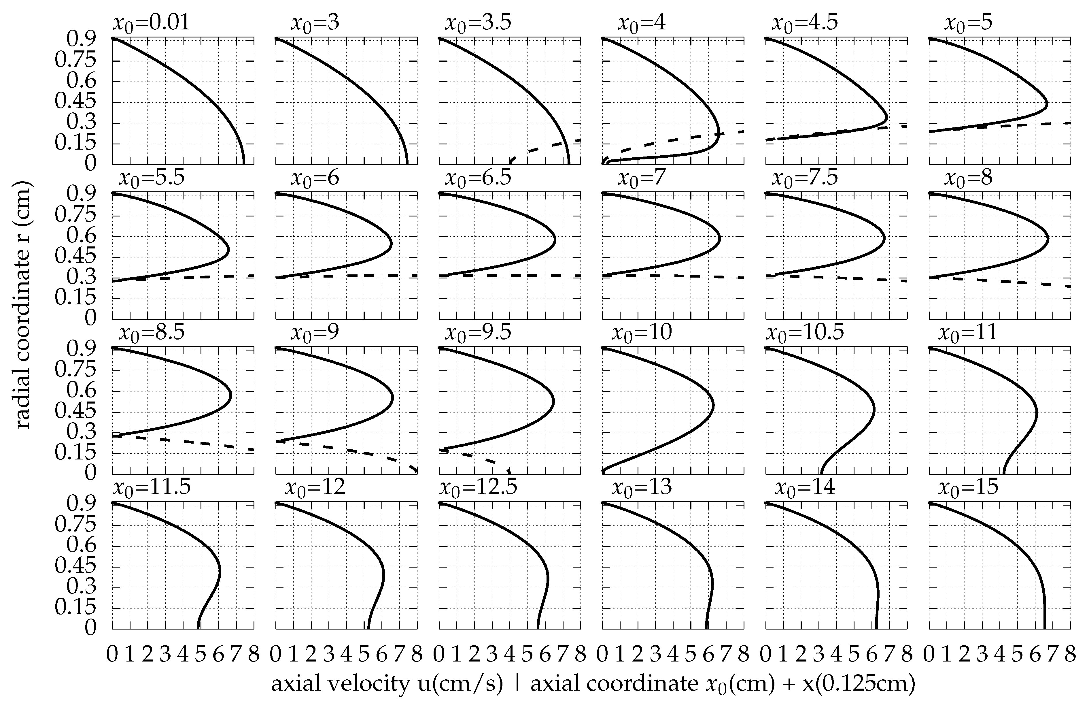
Appendix A. The Flow Field around the Balloon for Qin = 0.01 L/s, rb0 = 0.32 cm and Ab = 0.02 cm

The axial and radial velocity profiles for 4 instances in time and 24 axial positions is given in Figure A1, Figure A2, Figure A3, Figure A4, Figure A5, Figure A6, Figure A7 and Figure A8. Downstream of the intersection of the three perpendicular ellipsoid planes of symmetry, negative radial velocity component values emerge. The radial velocity component has its maximum in space at the point where the input stream attacks the balloon and in time at  t = T / 2  
max x , t U r ( x , 0 , θ , t ) = 2.17 cm / s .
The minimum in time, maximum value for the radial velocity emerges for  t = 6 T / 8  
min t max x U r ( x , 0 , θ , t ) = 1.88 cm / s .
For  x = 15  the maximum cross section axial velocity is on the pipe axis.
Figure A1. Axial velocity profiles for  t = 0 T / 8  (continuous line). The dashed line indicates the balloon profile. The inlet volume rate is  Q i n = 0.01  L/s,  r b 0 = 0.32  cm and  A b = 0.02  cm.
Fluids 08 00129 g0a1
Figure A2. Radial velocity profiles for  t = 0 T / 8  (continuous line). The dashed line indicates the balloon profile. The inlet volume rate is  Q i n = 0.01  L/s,  r b 0 = 0.32  cm and  A b = 0.02  cm.
Fluids 08 00129 g0a2
Figure A3. Axial velocity profiles for  t = 2 T / 8  (continuous line). The dashed line indicates the balloon profile. The inlet volume rate is  Q i n = 0.01  L/s,  r b 0 = 0.32  cm and  A b = 0.02  cm.
Fluids 08 00129 g0a3
Figure A4. Radial velocity profiles for  t = 2 T / 8  (continuous line). The dashed line indicates the balloon profile. The inlet volume rate is  Q i n = 0.01  L/s,  r b 0 = 0.32  cm and  A b = 0.02  cm.
Fluids 08 00129 g0a4
Figure A5. Axial velocity profiles for  t = 4 T / 8  (continuous line). The dashed line indicates the balloon profile. The inlet volume rate is  Q i n = 0.01  L/s,  r b 0 = 0.32  cm and  A b = 0.02  cm.
Fluids 08 00129 g0a5
Figure A6. Radial velocity profiles for  t = 4 T / 8  (continuous line). The dashed line indicates the balloon profile. The inlet volume rate is  Q i n = 0.01  L/s,  r b 0 = 0.32  cm and  A b = 0.02  cm.
Fluids 08 00129 g0a6
Figure A7. Axial velocity profiles for  t = 6 T / 8  (continuous line). The dashed line indicates the balloon profile. The inlet volume rate is  Q i n = 0.01  L/s,  r b 0 = 0.32  cm and  A b = 0.02  cm.
Fluids 08 00129 g0a7
Figure A8. Radial velocity profiles for  t = 6 T / 8  (continuous line). The dashed line indicates the balloon profile. The inlet volume rate is  Q i n = 0.01  L/s,  r b 0 = 0.32  cm and  A b = 0.02  cm.
Fluids 08 00129 g0a8

References

  1. McDonald, D.A. The relation of pulsatile pressure to flow in arteries. J. Physiol. 1955, 127, 533–552. [Google Scholar] [CrossRef] [PubMed]
  2. Womersley, J. Method for the calculation of velocity, rate of flow and viscous drag in arteries when the pressure gradient is known. J. Physiol. 1955, 127, 553–563. [Google Scholar] [CrossRef] [PubMed]
  3. Tsangaris, S.; Stergiopulos, N. The inverse Womersley problem for pulsatile flow in a straight rigid tube. J. Biomech. 1988, 21, 263–266. [Google Scholar] [CrossRef] [PubMed]
  4. Parissis, H.; Graham, V.; Lampridis, S.; Lau, M.; Hooks, G.; Mhandu, P. IABP: History-evolution-pathophysiology-indications: What we need to know. J. Cardiothorac. Surg. 2016, 11, 122. [Google Scholar] [CrossRef] [Green Version]
  5. Moulopoulos, S.; Topaz, S.; Kollf, W. Diastolic balloon pumping (with carbon dioxide) in the aorta—A mechanical assistance to the failing circulation. Am. Heart J. 1962, 5, 154–196. [Google Scholar] [CrossRef]
  6. Papaioannou, T.G.; Mathioulakis, D.S.; Nanas, J.N.; Tsangaris, S.G.; Stamatelopoulos, S.F.; Moulopoulos, S.D. Arterial compliance is a main variable determining the effectiveness of intra-aortic balloon counterpulsation: Quantitative data from an in vitro study. Med. Eng. Phys. 2002, 24, 279–284. [Google Scholar] [CrossRef]
  7. Papaioannou, T.; Mathioulakis, D.; Stamatelopoulos, K.; Giafalos, E.; Lekakis, J.; Nanas, J.; Stamatelopoulos, S.; Tsangaris, S. New aspects on the role of blood pressure and arterial stiffness in mechanical assistance by intra-aortic balloon pump: In-vitro data and their application in clinical practice. Artif. Organs 2004, 28, 717–727. [Google Scholar] [CrossRef]
  8. Xie, Y.; Yang, D.; Yu, H.; Wang, K.; Xie, Q. Development of Intra-Aortic Balloon Pump with Vascular Stent and Vitro Simulation Verification. In Proceedings of the 2021 IEEE 9th International Conference on Bioinformatics and Computational Biology, Taiyuan, China, 25–27 May 2021; pp. 174–179. [Google Scholar]
  9. Bruti, G. Experimental and Computational Investigations for the Development of Intra Aortic Balloon Pump Therapy. Ph.D. Thesis, Brunel University, London, UK, 2015. [Google Scholar]
  10. Gramigna, V.; Caruso, M.V.; Rossi, M.; Serraino, G.; Renzulli, A.; Fragomeni, G. A numerical analysis of the aortic blood flow pattern during pulsed cardiopulmonary bypass. Comput. Methods Biomech. Biomed. Eng. 2015, 18, 1574–1581. [Google Scholar] [CrossRef]
  11. Caruso, M.V.; Renzulli, A.; Fragomeni, G. Influence of IABP-Induced Abdominal Occlusions on Aortic Hemodynamics: A Patient-Specific Computational Evaluation. ASAIO J. 2017, 18, 161–167. [Google Scholar] [CrossRef]
  12. Caruso, M.V.; Gramigna, V.; Fragomeni, G. A CFD investigation of intra-aortic balloon pump assist ratio effects on aortic hemodynamics. Biocybernetics and Biomedical Engineering. ASAIO J. 2019, 39, 224–233. [Google Scholar]
  13. De Lazzari, B.; Badagliacca, R.; Filomena, D.; Papa, S.; Vizza, C.D.; Capoccia, M.; De Lazzari, C. CARDIOSIM: The First Italian Software Platform for Simulation of the Cardiovascular System and Mechanical Circulatory and Ventilatory Support. Bioengineering 2022, 9, 383. [Google Scholar] [CrossRef] [PubMed]
  14. De Lazzari, B.; Badagliacca, R.; Filomena, D.; Papa, S.; Vizza, C.D.; Capoccia, M.; De Lazzari, C. Intra-aortic balloon counterpulsation timing: A new numerical model for programming and training in the clinical environment. Comput. Methods Programs Biomed. 2020, 194, 150537. [Google Scholar] [CrossRef] [PubMed]
  15. Gu, K.; Guan, Z.; Lin, X.; Feng, Y.; Feng, J.; Yang, Y.; Zhang, Z.; Chang, Y.; Ling, Y.; Wan, F. Numerical analysis of aortic hemodynamics under the support of venoarterial extracorporeal membrane oxygenation and intra-aortic balloon pump. Comput. Methods Programs Biomed. 2019, 182, 105041. [Google Scholar] [CrossRef]
  16. Gu, K.; Gao, S.; Zhang, Z.; Ji, B.; Chang, Y. Hemodynamic Effect of Pulsatile on Blood Flow Distribution with VA ECMO: A Numerical Study. Bioengineering 2022, 9, 487. [Google Scholar] [CrossRef]
  17. Formaggia, L.; Quarteroni, A.; Veneziani, A. (Eds.) Cardiovascular Mathematics: Modeling and Simulation of the Circulatory System; Springer: Milan, Italy, 2009; Volume 1. [Google Scholar]
  18. Ahuja, S.; Bugliarello, G. A note on the compressibility of blood. Biorheology 1971, 7, 199–203. [Google Scholar] [CrossRef]
  19. Ge, L.; Sotiropoulos, F. A numerical method for solving the 3D unsteady incompressible Navier—Stokes equations in curvilinear domains with complex immersed boundaries. J. Comput. Phys. 2007, 225, 1782–1809. [Google Scholar] [CrossRef] [Green Version]
  20. Calderer, A.; Yang, X.; Angelidis, D.; Khosronejad, A.; Le, T.; Kang, S.; Gilmanov, A.; Ge, L.; Borazjani, I. Virtual Flow Simulator, Version 1.0; USDOE Office of Energy Efficiency and Renewable Energy (EERE): Golden, CO, USA, 2015.
  21. Moulinos, I.; Manopoulos, C.; Tsangaris, S. Computational Analysis of Active and Passive Flow Control for Backward Facing Step. Computation 2022, 10, 12. [Google Scholar] [CrossRef]
  22. Borazjani, I.; Ge, L.; Sotiropoulos, F. Curvilinear immersed boundary method for simulating fluid structure interaction with complex 3D rigid bodies. J. Comput. Phys. 2008, 227, 7587–7620. [Google Scholar] [CrossRef] [Green Version]
  23. Möller, T.; Trumbore, B. Fast, Minimum Storage Ray-Triangle Intersection. J. Graph. Tools 1997, 2, 21–28. [Google Scholar] [CrossRef]
  24. Yang, H.Q.; Habchi, S.D.; Przekwas, A.J. General strong conservation formulation of Navier-Stokes equations in nonorthogonal curvilinear coordinates. AIAA J. 1994, 32, 936–941. [Google Scholar] [CrossRef]
  25. Kang, S.K. Numerical Modeling of Turbulent Flows in Arbitrarily Complex Natural Streams. Ph.D. Thesis, University of Minnesota, Minneapolis, MN, USA, 2010. [Google Scholar]
  26. Calderer, A.; Kang, S.; Sotiropoulos, F. Level set immersed boundary method for coupled simulation of air/water interaction with complex floating structures. J. Comput. Phys. 2014, 277, 201–227. [Google Scholar] [CrossRef] [Green Version]
  27. Chorin, A.J. Numerical solutions of the Navier-Stokes equations. Math. Comput. 1968, 22, 745–762. [Google Scholar]
  28. Moré, J.J.; Sorensen, D.C.; Hillstrom, K.E.; Garbow, B.S. The MINPACK Project. In Sources and Development of Mathematical Software; Cowell, W.J., Ed.; Prentice-Hall: Hoboken, NJ, USA, 1984; pp. 88–111. [Google Scholar]
  29. Saad, Y.; Schultz, M.H. GMRES: A Generalized Minimal Residual Algorithm for Solving Nonsymmetric Linear Systems. SIAM J. Sci. Stat. Comput. 1986, 7, 856–869. [Google Scholar] [CrossRef] [Green Version]
  30. Ruge, J.W.; Stüben, K. Algebraic Multigrid. In Multigrid Methods; McCormick, S., Ed.; Society for Industrial and Applied Mathematics: Philadelphia, PA, USA, 1987; pp. 73–130. [Google Scholar]
  31. Cifu, D.X. (Ed.) Braddom’s Physical Medicine and Rehabilitation, 6th ed.; Elsevier: Amsterdam, The Netherlands, 2020. [Google Scholar]
  32. Hung, T.K. Unsteady flows with moving boundaries: Pulsating blood flows and earthquake hydrodynamics. In Advances in Engineering Mechanics—Reflections and Outlooks; World Scientific: Singapore, 2005; pp. 446–473. [Google Scholar]
  33. Tsangaris, S. Oscillatory flow of an incompressible, viscous fluid in a straight annular pipe. J. Méc.Théor. Appl. 1984, 3, 467–478. [Google Scholar]
  34. Zamir, M. The Physics of Coronary Blood Flow; AIP Press/Springer: New York, NY, USA, 2005. [Google Scholar]
  35. Nichols, W.; O’Rourke, M.; Elelman, E.; Vlachopoulos, C. (Eds.) McDonald’s Blood Flow in Arteries: Theoretical, Experimental and Clinical Principles, 7th ed.; CRC Press: Boca Raton, FL, USA, 2022. [Google Scholar]
  36. Uchida, S. The pulsating viscous flow superposed on the steady laminar motion of incompressible fluid in a circular pipe. Z. Angew. Math. Phys. 1956, 3, 403–422. [Google Scholar] [CrossRef]
  37. Westerhof, N.; Stergiopulos, N.; Noble, M.; Westerhof, B. Snapshots of Hemodynamics: An Aid for Clinical Research and Graduate Education; Springer: Cham, Switzerland, 2019. [Google Scholar]
  38. Verma, P.D. The pulsating viscous flow superposed on the steady laminar motion of incompressible fluid in a tube of elliptic section. Proc. Natl. Inst. Sci. India Part A 1960, 26, 282–297. [Google Scholar]
  39. Womersley, J.R. An Elastic Tube Theory of Pulse Transmission and Oscillatory Flow in Mammalian Arteries; TR 56-614; WADC: Fairborn, OH, USA, 1957. [Google Scholar]
Figure 1. Schematic of the prolate spheroid balloon and the coaxial to it, surrounding circular pipe.
Fluids 08 00129 g001
Figure 2. Inlet and outlet flow volume rate of the pipe for  Q i n = 0.01  L/s,  r b 0 = 0.32  cm and  A b = 0.02  cm.
Fluids 08 00129 g002
Figure 3. Decision of relative position of closed surface and underlying grid points in two-dimensional projection. A single ray is emitted from blocks ( i x , i y ) without intersection with the immersed boundary and a ray for each point of a block is emitted otherwise. The number of ray-immersed boundary intersections is noted in exemplary rays. Block (1,1): fluid, block (3,2): solid.
Fluids 08 00129 g003
Figure 4. Satisfaction of boundary condition on an immersed boundary node P. Velocity for P is estimated by linear interpolation between the velocity of the closest element C of the immersed surface and point A. Point A arises by extending the half line  C P  and finding its closest to P intersection with a triangle of fluid nodes. The example is presented in two dimensions for simplicity, i.e., the triangle of fluid nodes is represented by the line segment  B D .
Fluids 08 00129 g004
Figure 5. Surface grids of the prolate spheroid pulsating balloon and the circular pipe, along with their integration in the computational domain.
Fluids 08 00129 g005
Figure 6. Velocity vectors on a meridional plane, for a balloon pulsating according to Equation (4) with an inlet velocity profile given by Equation (18), for 8 instances during the period (left side titles refer to the fraction of the period T). The inlet volume rate is  Q i n = 0.01  L/s,  r b 0 = 0.36  cm and  A b = 0.06  cm.
Fluids 08 00129 g006
Figure 7. Velocity vectors on a meridional plane, for balloon pulsating according to Equation (4), with inlet velocity profile given by Equation (18), for 8 instances during the period (left side titles refer to the fraction of the period T). The inlet volume rate is  Q i n = 0.01  L/s,  r b 0 = 0.36  cm and  A b = 0.06  cm.
Fluids 08 00129 g007aFluids 08 00129 g007b
Figure 8. Radial velocity contours on a meridional plane, for balloon pulsating according to Equation (4) with inlet velocity profile given by Equation (18), for 8 instances during the period (left side titles refer to the fraction of the period T). The inlet volume rate is  Q i n = 0.01  L/s,  r b 0 = 0.36  cm and  A b = 0.06  cm.
Fluids 08 00129 g008aFluids 08 00129 g008b
Figure 9. Pressure on a meridional plane, for balloon pulsating according to Equation (4), with inlet velocity profile given by Equation (18), for 8 instances during the period (left side titles refer to the fraction of the period T). The inlet volume rate is  Q i n = 0.01  L/s,  r b 0 = 0.36  cm and  A b = 0.06  cm.
Fluids 08 00129 g009
Figure 10. Pressure  p o u t p i n  during a period for various values of  r b 0  and  A b .
Fluids 08 00129 g010
Figure 11. Outlet axial velocity profile  u o u t ( r )  sampled 8 times during the period. The inlet volume rate is  Q i n = 0.01  L/s,  r b 0 = 0.32  cm and  A b = 0.02  cm.
Fluids 08 00129 g011
Figure 12. Difference between outlet axial velocity profile  u o u t ( r )  and inlet axial velocity profile  u i n ( r ) , sampled 8 times during the period. The inlet volume rate is  Q i n = 0.01  L/s,  r b 0 = 0.32  cm and  A b = 0.02  cm.
Fluids 08 00129 g012
Table 1. Values of the geometric quantities of the simulation.
QuantityValue (cm)
r a 0.925
l a 18 (for  Q i n = 0.01  L/s), 40 (for  Q i n > 0.01  L/s)
α b 3
r b 0 0.32, 0.36, 0.44
A b 0.02, 0.06, 0.14
x l 7
Table 2. Values of the fluid properties in the CGS system of units.
QuantityValue
dynamic viscosity  μ 0.04 g/(cm·s)
density  ρ 1.06 g/cm3
Disclaimer/Publisher’s Note: The statements, opinions and data contained in all publications are solely those of the individual author(s) and contributor(s) and not of MDPI and/or the editor(s). MDPI and/or the editor(s) disclaim responsibility for any injury to people or property resulting from any ideas, methods, instructions or products referred to in the content.

