Artificial Neural Network Prediction of Minimum Fluidization Velocity for Mixtures of Biomass and Inert Solid Particles

Abstract

The fluidization of certain biomasses used in thermal processes, such as sawdust, is particularly difficult due to their irregular shapes, varied sizes, and low densities, causing high minimum fluidization velocities (U_mf). The addition of an inert material causes its U_mf to drop significantly. The determination of the U_mf of the binary mixture is however hard to obtain. Generally, predictive correlations are based on a small number of specific experiments, and sphericity is seldom included. In the present work, three models, i.e., an empirical correlation and two artificial neural networks (ANN) models were used to predict the U_mf of biomass-inert mixtures. An extensive bibliographical survey of more than 200 datasets was conducted with complete data about densities, particle diameters, sphericities, biomass fraction, and U_mf. With the combined application of the partial dependence plot (PDP) and the ANN models, the average effect of sphericity on U_mf was quantitatively determined (inverse relationship) together with the average impact of the biomass fraction on U_mf (direct relationship). In comparison with the empirical correlations, the results showed that both ANN models can accurately predict the U_mf of the presented binary mixtures with errors lower than 25%.

1. Introduction

The minimum fluidization velocity (U_mf) is an important hydrodynamic characteristic of gas–solid fluidized beds. It marks the transition from the fixed to the fluidized state and it is a crucial parameter in the design of reactors or other related devices based on the fluidized bed technology [1,2]. Although there is a large spectrum of correlations describing the minimum fluidization velocity for various binary mixtures of inert materials and biomass, they are empirical and only hold under certain specific conditions, reducing their applicability within narrow and defined boundary conditions. The use of these correlations in different scenarios leads to inaccuracies. A unified theoretical model could lead to predicting U_mf values more approximately. In most of the correlations developed to predict the U_mf of inert-biomass binary mixtures, the U_mf value depends on the effective density, the mean particle diameter, biomass fraction, and, in some cases, it also depends on the mean particle sphericity. In this context, a database obtained from the literature, used as a whole to be analyzed by artificial intelligence, can help to develop a comprehensive model that can be used to obtain better predictions compared to those obtained with existing correlations. Additionally, the same database can be used for the development of a general and accurate correlation.

In this context, the objectives of this work consist of, first, building a comprehensive database obtained from an extensive literature survey of the minimum fluidization velocities of inert-biomass binary mixtures. Second, using those datasets to develop an empirical correlation and train two ANN models all of which encompass and unify a large spectrum of experimental data. Then, using the developed models to determine the impact the independent variables have on the U_mf value, and, finally, to compare the accuracy of the three models.

2. Background

For binary mixtures of biomass and inert materials, the inert material generally fluidizes at a lower gas flow rate than the biomass. These systems present segregation and, in general, the inert material with a higher density than the biomass tends to descend into the bed. In systems where there is no density difference, the larger particles tend to descend. Based on the degree of mixing/segregation of binary systems, [3] they are classified as (i) complete mixing, (ii) complete segregation, and (iii) partial mixing. The first case occurs when the binary system does not have a large difference in size and density. In case (ii), two zones are clearly distinguished, one in the lower part, where the inert material is found, and the other one in the upper part, where the biomass component is located. Case (iii) is an intermediate case between the previous ones. This is the predominant behavior in biomass-inert fluidized beds of interest in this work. For each one of these cases, the determination of U_mf is based on the curve ΔP vs. U obtained during the defluidization of the system [4].

2.1. Minimum Fluidization Velocity of Binary Mixtures

Many authors have studied the fluid-dynamic behavior of inert-biomass mixtures during fluidization in recent decades. Among them, the works of [5,6,7,8,9,10,11,12,13,14,15] focus on evaluating the quality of fluidization and the accuracy of different correlations to predict the minimum fluidization velocity of mixtures at different proportions and under different operating conditions. However, the development of such correlations dates back to the early 1970s. The most relevant works on the subject are summarized below, and the corresponding correlations are presented in Table 1. The subscripts P and F used in the equations presented in Table 1 correspond to biomass and inert, respectively, and coincide with those used by [3].

Goossens et al. [16] modified the equation of Wen and Yu [17] to determine the U_mf of monodisperse systems. To employ this correlation, the authors defined equations to evaluate the average diameter and density of binary mixtures as a function of the diameters, densities, and weight fractions of each component.

Cheung, Nienow, and Rowe [18] developed a correlation to estimate U_mf in binary mixtures of particles of different diameters with the same density and shape. Its correlation allows the U_mf value of the mixture to be determined from the values of the minimum fluidization velocity of each group of particles and their composition (weight fraction of the particles with the largest diameter). This work was continued by [19] who worked with particle systems of the same density and shape, although these systems were formed by mixtures of two, three, and five different diameters. The authors presented a semi-empirical correlation also considering the pressure loss equation through a porous medium from [20], in which the value of U_mf for the mixture of solids with more than two different diameters is a function of the porosity of a bed made up of particles of a single diameter (the largest or the smallest) and the respective U_mf value.

Chiba et al. [3] developed correlations for the cases of completely mixed binary mixtures and for completely segregated mixtures. The authors measured the pressure drop in the bed after quickly (maximum mixing condition) and slowly (highest degree of segregation) defluidizing the system. In the first case, the correlation requires knowledge of the minimum fluidization velocity of the component that fluidizes at a lower superficial gas velocity (the fluid component) and of the diameter and density of the mixture. In the case of completely segregated mixtures, it is necessary to know the velocity of the fluid component and of the component that fluidizes at the highest value of superficial velocity (the packed component).

Noda et al. [21] studied the fluidization of mixtures of large particles (including wood chip particles) and small ones of different densities. The authors determined correlations for parameters A and B of the Ergun equation [22] modified by Wen and Yu [17]. The parameters depend on the composition of the binary mixture and the ratio between the diameters and the densities of the components. The diameter and density of the solid mixture were determined using the equations of Goossens [16]. Based on their results, the authors concluded that the minimum fluidization velocity of the binary mixtures studied strongly depends on the mixing conditions, determined by the pair of densities, and on the volume fraction of the component that fluidizes at the velocity value of lower gas.

Bilbao et al. [23] worked with binary mixtures of sand and straw. In their experiments, they used different diameters, both for the inert and for the biomass, evaluating in each case the maximum volume fraction of straw that would allow for maintaining the fluidization quality. In this sense, the authors developed a correlation to evaluate the minimum volumetric fraction of sand necessary to carry out fluidization. They also proposed a correlation based on the minimum fluidization velocities of the sand and straw particles and the real sand volume fraction in the bed defined (those which would correspond to zero porosity). The authors proposed the use of the correlation of Wen and Yu [17] to calculate the minimum fluidization velocity of sand, and a correlation adjusted with their data to evaluate the minimum fluidization velocity of straw from the diameter of the particles.

Rao and Bheemarasetti [24] carried out studies on the fluidization of mixtures of biomass and sands. The biomass materials used were rice husk, sawdust, and groundnut shell powder, and the sands employed were of two different densities and particle sizes. To evaluate the U_mf of the mixtures, they used the Ergun correlation [22], simplified for the special case of very small particles [25], together with an empirical correlation to evaluate the effective diameter and the equation defined by Goossens [16] to determine the mean mixing density.

Zhong et al. [26] studied the fluidization of biomass particles and binary mixtures of biomass particles with different fluidization mediums. The biomass particles used were wood chips, mung beans, millet, corn stalk, and cotton stalk, and the fluidization mediums employed were silica sand, continental flood basalt (CFB) cinder, and aluminum oxide. Based on the general expression proposed by [27] for single particle systems, the authors determined two correlations to predict the minimum fluidization velocity of binary mixtures, one of them for a low-effective density particulate system (0 < $\bar{\mathsf{\rho }}$ ≤ 1000 kg/m³), and the other one, for the high-effective density particulate system ($\bar{\mathsf{\rho }}$ > 1000 kg/m³).

Si and Guo [28] investigated the fluidization of binary mixtures in an acoustic bubbling fluidized bed. In their experiments, they used two types of biomass particles, sawdust and wheat stalk. The authors developed a correlation to predict U_mf for mixtures of biomass and sand based on effective properties determined from the equations proposed by Goosens [16]. Although the correlation developed has the form of the equation of Wen and Yu [17], an aspect to highlight in the work is that the coefficients A and B are considered as a function of the sphericity values of the particles.

Oliveira et al. [29] studied the fluidization of mixtures of biomass and sand. In their experiments, they worked with three types of biomasses (sweet sorghum bagasse, waste tobacco, and soybean hulls) and four sizes of sand particles, forming mixtures in different proportions. The authors presented a predictive correlation of the minimum fluidization velocity for mixtures of biomass and inert material from the function originally proposed by [27] for single-particle systems.

Shao et al. [30] carried out experiments with mixtures of silica sand and four types of particles differing in shapes, sizes, and densities (biomass waste and plastic materials). The pressure drop, flow pattern, and minimum fluidization velocity under different operating conditions were investigated by recording pressure differential signals and fluidization images.

Paudel and Feng [31] studied the fluidization of biomass particles (corn cobs and walnut shells), inert particles (sand, glass beads, and alumina), and biomass and sand mixtures. For the experiments with mixtures, they used biomass in mass percentages between 0–100%. Based on their experimental results, they determined a new correlation to predict the values of minimum fluidization velocity of inerts, biomass, and mixtures of both. The correlation depends on the Archimedes number, on effective properties determined from the equations of Goosens [16], and on the weight fraction of the biomass used. The zero value in the variable allows us to evaluate the minimum fluidization velocity of the inert material, and the value of the variable in one allows us to predict the minimum fluidization velocity of the pure biomass.

A relevant work on the subject is that of Kumoro et al. [32], who developed a correlation from the equation of Wen and Yu [17], considering the coefficients A and B as functions of the effective sphericity and the weight fraction of the biomass. Rice husk and corn cob particles were used as biomass along with two types of sand as inert material. In its correlation, the minimum fluidization velocity depends on the Archimedes number, evaluated from the effective properties of the mixture. The density of the sand-biomass mixtures was calculated using the equation of Rao and Bheemarasetti [24], the average particle diameter was calculated using the equation developed by [16], and the mean sphericity of the particle mixture was evaluated using the equation suggested by [33].

More recently, Reyes-Urrutia et al. [34] analyzed the influence of different definitions for evaluating the sphericity factor on the prediction of minimum fluidization velocity of different agro-industrial/forestry biomass residues and sand. Three types of biowastes (sawdust, grape marc, and grape stalk) and sand were characterized by sieving, and sphericity was calculated using images obtained by scanning electron microscopy (SEM). Sand particles, with a mean diameter of 0.33 mm, were used as inert material. Riley’s sphericity method proved to be the most suitable. Finally, a new correlation to evaluate U_mf was proposed for biomass-inert particle binary systems.

Table 1. Modeling minimum fluidization velocities of binary mixtures.

References	Correlations		Additional Equations
[16]	${\mathrm{Re}}_{\mathrm{mf}}={\left({33.7}^2+0.0408\times \mathrm{Ar}\right)}^{1/2}-33.7$	(1)	$\frac{1}{\bar{\mathsf{\rho }}}=\frac{{\mathrm{x}}_{\mathrm{F}}}{{\mathsf{\rho }}_{\mathrm{F}}}+\frac{1-{\mathrm{x}}_{\mathrm{F}}}{{\mathsf{\rho }}_{\mathrm{P}}}$	(16)
			$\bar{\mathrm{d}}={\mathrm{d}}_{\mathrm{F}}{\mathrm{d}}_{\mathrm{P}}\frac{\left(1-{\mathrm{x}}_{\mathrm{F}}\right){\mathsf{\rho }}_{\mathrm{F}}+{\mathrm{x}}_{\mathrm{F}}{\mathsf{\rho }}_{\mathrm{P}}}{\left(1-{\mathrm{x}}_{\mathrm{F}}\right){\mathsf{\rho }}_{\mathrm{F}}{\mathrm{d}}_{\mathrm{F}}+{\mathrm{x}}_{\mathrm{F}}{\mathsf{\rho }}_{\mathrm{P}}{\mathrm{d}}_{\mathrm{P}}}$	(17)
[18]	$\frac{{\mathrm{U}}_{\mathrm{mf}}}{{\mathrm{U}}_{\mathrm{S}}}={\left(\frac{{\mathrm{U}}_{\mathrm{B}}}{{\mathrm{U}}_{\mathrm{s}}}\right)}^{{{\mathrm{x}}_{\mathrm{B}}}^2}, \frac{{\mathrm{d}}_{\mathrm{B}}}{{\mathrm{d}}_{\mathrm{s}}}<3 \wedge \frac{{\mathrm{U}}_{\mathrm{B}}}{{\mathrm{U}}_{\mathrm{s}}}<10$	(2)
[3]	For the completely mixed bed ${\mathrm{U}}_{\mathrm{mf}}={\mathrm{U}}_{\mathrm{F}}\frac{\bar{\mathsf{\rho }}}{{\mathsf{\rho }}_{\mathrm{F}}}{\left(\frac{\bar{\mathrm{d}}}{{\mathrm{d}}_{\mathrm{F}}}\right)}^2$ For the completely segregated bed ${\mathrm{U}}_{\mathrm{mf}}=\frac{{\mathrm{U}}_{\mathrm{F}}}{\left(1-{\mathrm{U}}_{\mathrm{F}}/{\mathrm{U}}_{\mathrm{P}}\right){\mathrm{x}}_{\mathrm{F}}+{\mathrm{U}}_{\mathrm{F}}/{\mathrm{U}}_{\mathrm{P}}}$	(3)	$\bar{\mathsf{\rho }}={\mathrm{f}}_{\mathrm{F}}{ \mathsf{\rho }}_{\mathrm{F}}+\left(1-{\mathrm{f}}_{\mathrm{F}}\right){\mathsf{\rho }}_{\mathrm{P}}$	(18)
			$\bar{\mathrm{d}}={\left[{\mathrm{f}}_{\mathrm{N}}{\mathrm{d}}_{\mathrm{F}}^3+\left(1-{\mathrm{f}}_{\mathrm{N}}{\mathrm{d}}_{\mathrm{P}}^3\right)\right]}^{1/3}$	(19)
		(4)	${\mathrm{f}}_{\mathrm{N}}=\frac{1}{\left[1+\left(\frac{1}{{\mathrm{f}}_{\mathrm{F}}}-1\right){\left(\frac{{\mathrm{d}}_{\mathrm{F}}}{{\mathrm{d}}_{\mathrm{P}}}\right)}^3\right]}$	(20)
[21]	$\mathrm{A}\mathrm{r}=\mathrm{A} {\mathrm{R}\mathrm{e}}_{\mathrm{m}\mathrm{f}}^2+\mathrm{B} {\mathrm{R}\mathrm{e}}_{\mathrm{m}\mathrm{f}}$	(5)	$\bar{\mathsf{\rho }}$, Equation (16)
			$\bar{\mathrm{d}}$, Equation (17)
			$\mathrm{A}=36.2{\left(\frac{{\mathrm{d}}_{\mathrm{P}}}{{\mathrm{d}}_{\mathrm{F}}}\frac{{\mathsf{\rho }}_{\mathrm{F}}}{{\mathsf{\rho }}_{\mathrm{P}}}\right)}^{-0.196}$	(21)
			when the bed is completely mixed after both components are fluidized $\mathrm{B}=1397 {\left(\frac{{\mathrm{d}}_{\mathrm{P}}}{{\mathrm{d}}_{\mathrm{F}}}\frac{{\mathsf{\rho }}_{\mathrm{F}}}{{\mathsf{\rho }}_{\mathrm{P}}}\right)}^{0.296}$	(22)
			when the bed is partially mixed after both components are fluidized, and $\frac{{\mathrm{d}}_{\mathrm{P}}}{{\mathrm{d}}_{\mathrm{F}}}>3$ and $\frac{{\mathsf{\rho }}_{\mathrm{F}}}{{\mathsf{\rho }}_{\mathrm{P}}}\approx 1$ $\mathrm{B}=6443 {\left(\frac{{\mathrm{d}}_{\mathrm{P}}}{{\mathrm{d}}_{\mathrm{F}}}\frac{{\mathsf{\rho }}_{\mathrm{F}}}{{\mathsf{\rho }}_{\mathrm{P}}}\right)}^{-1.86}$	(23)
[23]	${\mathrm{U}}_{\mathrm{v},\mathrm{f}}={\mathrm{U}}_{\mathrm{P},\mathrm{f}}-\left({\mathrm{U}}_{\mathrm{P},\mathrm{f}}-{\mathrm{U}}_{\mathrm{F}}\right){\mathrm{f}}_{\mathrm{F},\mathrm{Real}}$	(6)	${\mathrm{f}}_{\mathrm{F},\mathrm{Real}}=\frac{{\mathrm{x}}_{\mathrm{F}}}{{\mathrm{x}}_{\mathrm{F}}+\frac{{\mathsf{\rho }}_{\mathrm{F}}}{{\mathsf{\rho }}_{\mathrm{P}}}\left(1-{\mathrm{x}}_{\mathrm{F}}\right)}$	(24)
			${\mathrm{U}}_{\mathrm{P},\mathrm{f}}=50{\mathrm{d}}_{\mathrm{P}}^{0.84}$	(25)
			For determinate UF ${\mathrm{Re}}_{\mathrm{mf}}=\sqrt{{\mathrm{A}}^2+\mathrm{B} \mathrm{Ar}}-\mathrm{A}$	(26)
[24]	${\mathrm{U}}_{\mathrm{mf}}=\frac{{\bar{\mathrm{d}}}^2\left(\bar{\mathsf{\rho }}-{\mathsf{\rho }}_{\mathrm{g}}\right)\mathrm{g}}{1650{\mu }_{\mathrm{g}}}$	(7)	$\bar{\mathsf{\rho }}={\mathrm{x}}_{\mathrm{F}}{\mathsf{\rho }}_{\mathrm{F}}+{\mathrm{x}}_{\mathrm{P}}{\mathsf{\rho }}_{\mathrm{P}}$	(27)
			${\bar{\mathrm{d}}}^2={\mathrm{k}}^{\prime }{\left\{{\mathrm{d}}_{\mathrm{F}}{\left[\left(\frac{{\mathsf{\rho }}_{\mathrm{F}}}{{\mathsf{\rho }}_{\mathrm{P}}}\right)\left(\frac{{\mathrm{d}}_{\mathrm{P}}}{{\mathrm{d}}_{\mathrm{F}}}\right)\right]}^{{\mathrm{w}}_{\mathrm{P}}/{\mathrm{w}}_{\mathrm{F}}}\right\}}^2$	(28)
			${\mathrm{k}}^{\prime }=20{\mathrm{d}}_{\mathrm{F}}+0.36$	(29)
[26]	${\mathrm{U}}_{\mathrm{mf}}=1.2\times {10}^{-4}{\left[\frac{{\bar{\mathrm{d}}}^2\left(\bar{\mathsf{\rho }}-{\mathsf{\rho }}_{\mathrm{g}}\right)}{{\mu }_{\mathrm{g}}}{\left(\frac{\bar{\mathsf{\rho }}}{{\mathsf{\rho }}_{\mathrm{g}}}\right)}^{1.23}\right]}^{0.633}$ for $0<\bar{\mathsf{\rho }}\le 1000 \mathrm{kg}/{\mathrm{cm}}^3$	(8)	$\bar{\mathsf{\rho }}$, Equation (27)
	${\mathrm{U}}_{\mathrm{mf}}=1.45\times {10}^{-3}{\left[\frac{{\bar{\mathrm{d}}}^2\left(\bar{\mathsf{\rho }}-{\mathsf{\rho }}_{\mathrm{g}}\right)}{{\mu }_{\mathrm{g}}}{\left(\frac{\bar{\mathsf{\rho }}}{{\mathsf{\rho }}_{\mathrm{g}}}\right)}^{1.23}\right]}^{0.363}$ for $\bar{\mathsf{\rho }}\ge 1000\mathrm{kg}/{\mathrm{cm}}^3$	(9)	$\bar{\mathrm{d}}={\mathrm{d}}_1{\left[\left(\frac{{\mathsf{\rho }}_1}{{\mathsf{\rho }}_2}\right)\left(\frac{{\mathrm{d}}_2}{{\mathrm{d}}_1}\right)\right]}^{{\mathrm{x}}_2/{\mathrm{x}}_1}$ $1$ correspond to the particle that is in less mass fraction of the mixture	(30)
[28]	${\mathrm{Re}}_{\mathrm{mf}}={\left({\mathrm{A}}^2+\mathrm{B} \mathrm{Ar}\right)}^{1/2}-\mathrm{A}$	(10)	$\mathrm{A}=25.65\left({\mathsf{\varphi }}_{\mathrm{P}}^{0.21}{\mathsf{\varphi }}_{\mathrm{F}}^{0.15}\right)$	(31)
			$\mathrm{B}=0.056\left({\mathsf{\varphi }}_{\mathrm{P}}^{-0.045}{\mathsf{\varphi }}_{\mathrm{F}}^{0.015}\right)$	(32)
[30]	${\mathrm{U}}_{\mathrm{mf}}=1.28\times {10}^{-3}{\left[\frac{{\bar{\mathrm{d}}}^2\left(\bar{\mathsf{\rho }}-{\mathsf{\rho }}_{\mathrm{g}}\right)\mathrm{g}}{{\mu }_{\mathrm{g}}}{\left(\frac{\bar{\mathsf{\rho }}}{{\mathsf{\rho }}_{\mathrm{g}}}\right)}^{1.2}\right]}^{0.356}$	(11)	$\bar{\mathsf{\rho }}$, Equation (27)
			$\bar{\mathrm{d}}={\mathrm{d}}_{\mathrm{F}}{\left[\left(\frac{{\mathsf{\rho }}_{\mathrm{F}}}{{\mathsf{\rho }}_{\mathrm{P}}}\right)\left(\frac{{\mathrm{d}}_{\mathrm{P}}}{{\mathrm{d}}_{\mathrm{F}}}\right)\right]}^{{\mathrm{x}}_{\mathrm{P}}/{\mathrm{x}}_{\mathrm{F}}}$	(33)
[31]	${\mathrm{Re}}_{\mathrm{mf}}={\left\{{30.28}^2+\left[0.046\left(1-{\mathrm{x}}_{\mathrm{P}}\right)+0.108{\mathrm{x}}_{\mathrm{P}}^{1/2}\right]\mathrm{Ar}\right\}}^{1/2}-30.28$	(12)	$\stackrel{-}{\mathsf{\rho }}$, Equation (16)
			$\stackrel{-}{\mathrm{d}}$, Equation (17)
[29]	${\mathrm{U}}_{\mathrm{mf}}=\left(1.17\times {10}^{-4}\pm 6\times {10}^{-5}\right){\left[\frac{{\bar{\mathrm{d}}}^2\left(\bar{\mathsf{\rho }}-{\mathsf{\rho }}_{\mathrm{g}}\right)\mathrm{g}}{{\mu }_{\mathrm{g}}}{\left(\frac{\bar{\mathsf{\rho }}}{{\mathsf{\rho }}_{\mathrm{g}}}\right)}^{1.23}\right]}^{0.4916\pm 0.032}$	(13)	$\bar{\mathsf{\rho }}$, Equation (27)
			$\bar{\mathrm{d}}$, Equation (33)
[32]	$\mathrm{Ar}=1176 \left(1-{\mathrm{x}}_{\mathrm{P}}\right){\bar{\mathsf{\varphi }}}^2{\mathrm{Re}}_{\mathrm{mf}}+22.432 {\mathrm{x}}_{\mathrm{P}}^{1/2}{\mathrm{Re}}_{\mathrm{mf}}^2$	(14)	$\bar{\mathsf{\rho }}$, Equation (27)
			$\stackrel{-}{\mathrm{d}}$, Equation (17)
			$\bar{\mathsf{\varphi }}={\mathrm{x}}_{\mathrm{F}}{\mathsf{\varphi }}_{\mathrm{F}}+{\mathrm{x}}_{\mathrm{P}}{\mathsf{\varphi }}_{\mathrm{P}}$	(34)
[34]	${\mathrm{Re}}_{\mathrm{mf}}=0.1(1-\bar{\mathsf{\varphi }}){\mathrm{Ar}}^{0.616}$	(15)	$\stackrel{-}{\mathsf{\rho }}$, Equation (16)
			$\stackrel{-}{\mathrm{d}}$, Equation (17)
			$\stackrel{-}{\mathsf{\varphi }}$, Equation (34)

Table 1. Modeling minimum fluidization velocities of binary mixtures.

References	Correlations		Additional Equations
[16]	${\mathrm{Re}}_{\mathrm{mf}}={\left({33.7}^2+0.0408\times \mathrm{Ar}\right)}^{1/2}-33.7$	(1)	$\frac{1}{\bar{\mathsf{\rho }}}=\frac{{\mathrm{x}}_{\mathrm{F}}}{{\mathsf{\rho }}_{\mathrm{F}}}+\frac{1-{\mathrm{x}}_{\mathrm{F}}}{{\mathsf{\rho }}_{\mathrm{P}}}$	(16)
			$\bar{\mathrm{d}}={\mathrm{d}}_{\mathrm{F}}{\mathrm{d}}_{\mathrm{P}}\frac{\left(1-{\mathrm{x}}_{\mathrm{F}}\right){\mathsf{\rho }}_{\mathrm{F}}+{\mathrm{x}}_{\mathrm{F}}{\mathsf{\rho }}_{\mathrm{P}}}{\left(1-{\mathrm{x}}_{\mathrm{F}}\right){\mathsf{\rho }}_{\mathrm{F}}{\mathrm{d}}_{\mathrm{F}}+{\mathrm{x}}_{\mathrm{F}}{\mathsf{\rho }}_{\mathrm{P}}{\mathrm{d}}_{\mathrm{P}}}$	(17)
[18]	$\frac{{\mathrm{U}}_{\mathrm{mf}}}{{\mathrm{U}}_{\mathrm{S}}}={\left(\frac{{\mathrm{U}}_{\mathrm{B}}}{{\mathrm{U}}_{\mathrm{s}}}\right)}^{{{\mathrm{x}}_{\mathrm{B}}}^2}, \frac{{\mathrm{d}}_{\mathrm{B}}}{{\mathrm{d}}_{\mathrm{s}}}<3 \wedge \frac{{\mathrm{U}}_{\mathrm{B}}}{{\mathrm{U}}_{\mathrm{s}}}<10$	(2)
[3]	For the completely mixed bed ${\mathrm{U}}_{\mathrm{mf}}={\mathrm{U}}_{\mathrm{F}}\frac{\bar{\mathsf{\rho }}}{{\mathsf{\rho }}_{\mathrm{F}}}{\left(\frac{\bar{\mathrm{d}}}{{\mathrm{d}}_{\mathrm{F}}}\right)}^2$ For the completely segregated bed ${\mathrm{U}}_{\mathrm{mf}}=\frac{{\mathrm{U}}_{\mathrm{F}}}{\left(1-{\mathrm{U}}_{\mathrm{F}}/{\mathrm{U}}_{\mathrm{P}}\right){\mathrm{x}}_{\mathrm{F}}+{\mathrm{U}}_{\mathrm{F}}/{\mathrm{U}}_{\mathrm{P}}}$	(3)	$\bar{\mathsf{\rho }}={\mathrm{f}}_{\mathrm{F}}{ \mathsf{\rho }}_{\mathrm{F}}+\left(1-{\mathrm{f}}_{\mathrm{F}}\right){\mathsf{\rho }}_{\mathrm{P}}$	(18)
			$\bar{\mathrm{d}}={\left[{\mathrm{f}}_{\mathrm{N}}{\mathrm{d}}_{\mathrm{F}}^3+\left(1-{\mathrm{f}}_{\mathrm{N}}{\mathrm{d}}_{\mathrm{P}}^3\right)\right]}^{1/3}$	(19)
		(4)	${\mathrm{f}}_{\mathrm{N}}=\frac{1}{\left[1+\left(\frac{1}{{\mathrm{f}}_{\mathrm{F}}}-1\right){\left(\frac{{\mathrm{d}}_{\mathrm{F}}}{{\mathrm{d}}_{\mathrm{P}}}\right)}^3\right]}$	(20)
[21]	$\mathrm{A}\mathrm{r}=\mathrm{A} {\mathrm{R}\mathrm{e}}_{\mathrm{m}\mathrm{f}}^2+\mathrm{B} {\mathrm{R}\mathrm{e}}_{\mathrm{m}\mathrm{f}}$	(5)	$\bar{\mathsf{\rho }}$, Equation (16)
			$\bar{\mathrm{d}}$, Equation (17)
			$\mathrm{A}=36.2{\left(\frac{{\mathrm{d}}_{\mathrm{P}}}{{\mathrm{d}}_{\mathrm{F}}}\frac{{\mathsf{\rho }}_{\mathrm{F}}}{{\mathsf{\rho }}_{\mathrm{P}}}\right)}^{-0.196}$	(21)
			when the bed is completely mixed after both components are fluidized $\mathrm{B}=1397 {\left(\frac{{\mathrm{d}}_{\mathrm{P}}}{{\mathrm{d}}_{\mathrm{F}}}\frac{{\mathsf{\rho }}_{\mathrm{F}}}{{\mathsf{\rho }}_{\mathrm{P}}}\right)}^{0.296}$	(22)
			when the bed is partially mixed after both components are fluidized, and $\frac{{\mathrm{d}}_{\mathrm{P}}}{{\mathrm{d}}_{\mathrm{F}}}>3$ and $\frac{{\mathsf{\rho }}_{\mathrm{F}}}{{\mathsf{\rho }}_{\mathrm{P}}}\approx 1$ $\mathrm{B}=6443 {\left(\frac{{\mathrm{d}}_{\mathrm{P}}}{{\mathrm{d}}_{\mathrm{F}}}\frac{{\mathsf{\rho }}_{\mathrm{F}}}{{\mathsf{\rho }}_{\mathrm{P}}}\right)}^{-1.86}$	(23)
[23]	${\mathrm{U}}_{\mathrm{v},\mathrm{f}}={\mathrm{U}}_{\mathrm{P},\mathrm{f}}-\left({\mathrm{U}}_{\mathrm{P},\mathrm{f}}-{\mathrm{U}}_{\mathrm{F}}\right){\mathrm{f}}_{\mathrm{F},\mathrm{Real}}$	(6)	${\mathrm{f}}_{\mathrm{F},\mathrm{Real}}=\frac{{\mathrm{x}}_{\mathrm{F}}}{{\mathrm{x}}_{\mathrm{F}}+\frac{{\mathsf{\rho }}_{\mathrm{F}}}{{\mathsf{\rho }}_{\mathrm{P}}}\left(1-{\mathrm{x}}_{\mathrm{F}}\right)}$	(24)
			${\mathrm{U}}_{\mathrm{P},\mathrm{f}}=50{\mathrm{d}}_{\mathrm{P}}^{0.84}$	(25)
			For determinate UF ${\mathrm{Re}}_{\mathrm{mf}}=\sqrt{{\mathrm{A}}^2+\mathrm{B} \mathrm{Ar}}-\mathrm{A}$	(26)
[24]	${\mathrm{U}}_{\mathrm{mf}}=\frac{{\bar{\mathrm{d}}}^2\left(\bar{\mathsf{\rho }}-{\mathsf{\rho }}_{\mathrm{g}}\right)\mathrm{g}}{1650{\mu }_{\mathrm{g}}}$	(7)	$\bar{\mathsf{\rho }}={\mathrm{x}}_{\mathrm{F}}{\mathsf{\rho }}_{\mathrm{F}}+{\mathrm{x}}_{\mathrm{P}}{\mathsf{\rho }}_{\mathrm{P}}$	(27)
			${\bar{\mathrm{d}}}^2={\mathrm{k}}^{\prime }{\left\{{\mathrm{d}}_{\mathrm{F}}{\left[\left(\frac{{\mathsf{\rho }}_{\mathrm{F}}}{{\mathsf{\rho }}_{\mathrm{P}}}\right)\left(\frac{{\mathrm{d}}_{\mathrm{P}}}{{\mathrm{d}}_{\mathrm{F}}}\right)\right]}^{{\mathrm{w}}_{\mathrm{P}}/{\mathrm{w}}_{\mathrm{F}}}\right\}}^2$	(28)
			${\mathrm{k}}^{\prime }=20{\mathrm{d}}_{\mathrm{F}}+0.36$	(29)
[26]	${\mathrm{U}}_{\mathrm{mf}}=1.2\times {10}^{-4}{\left[\frac{{\bar{\mathrm{d}}}^2\left(\bar{\mathsf{\rho }}-{\mathsf{\rho }}_{\mathrm{g}}\right)}{{\mu }_{\mathrm{g}}}{\left(\frac{\bar{\mathsf{\rho }}}{{\mathsf{\rho }}_{\mathrm{g}}}\right)}^{1.23}\right]}^{0.633}$ for $0<\bar{\mathsf{\rho }}\le 1000 \mathrm{kg}/{\mathrm{cm}}^3$	(8)	$\bar{\mathsf{\rho }}$, Equation (27)
	${\mathrm{U}}_{\mathrm{mf}}=1.45\times {10}^{-3}{\left[\frac{{\bar{\mathrm{d}}}^2\left(\bar{\mathsf{\rho }}-{\mathsf{\rho }}_{\mathrm{g}}\right)}{{\mu }_{\mathrm{g}}}{\left(\frac{\bar{\mathsf{\rho }}}{{\mathsf{\rho }}_{\mathrm{g}}}\right)}^{1.23}\right]}^{0.363}$ for $\bar{\mathsf{\rho }}\ge 1000\mathrm{kg}/{\mathrm{cm}}^3$	(9)	$\bar{\mathrm{d}}={\mathrm{d}}_1{\left[\left(\frac{{\mathsf{\rho }}_1}{{\mathsf{\rho }}_2}\right)\left(\frac{{\mathrm{d}}_2}{{\mathrm{d}}_1}\right)\right]}^{{\mathrm{x}}_2/{\mathrm{x}}_1}$ $1$ correspond to the particle that is in less mass fraction of the mixture	(30)
[28]	${\mathrm{Re}}_{\mathrm{mf}}={\left({\mathrm{A}}^2+\mathrm{B} \mathrm{Ar}\right)}^{1/2}-\mathrm{A}$	(10)	$\mathrm{A}=25.65\left({\mathsf{\varphi }}_{\mathrm{P}}^{0.21}{\mathsf{\varphi }}_{\mathrm{F}}^{0.15}\right)$	(31)
			$\mathrm{B}=0.056\left({\mathsf{\varphi }}_{\mathrm{P}}^{-0.045}{\mathsf{\varphi }}_{\mathrm{F}}^{0.015}\right)$	(32)
[30]	${\mathrm{U}}_{\mathrm{mf}}=1.28\times {10}^{-3}{\left[\frac{{\bar{\mathrm{d}}}^2\left(\bar{\mathsf{\rho }}-{\mathsf{\rho }}_{\mathrm{g}}\right)\mathrm{g}}{{\mu }_{\mathrm{g}}}{\left(\frac{\bar{\mathsf{\rho }}}{{\mathsf{\rho }}_{\mathrm{g}}}\right)}^{1.2}\right]}^{0.356}$	(11)	$\bar{\mathsf{\rho }}$, Equation (27)
			$\bar{\mathrm{d}}={\mathrm{d}}_{\mathrm{F}}{\left[\left(\frac{{\mathsf{\rho }}_{\mathrm{F}}}{{\mathsf{\rho }}_{\mathrm{P}}}\right)\left(\frac{{\mathrm{d}}_{\mathrm{P}}}{{\mathrm{d}}_{\mathrm{F}}}\right)\right]}^{{\mathrm{x}}_{\mathrm{P}}/{\mathrm{x}}_{\mathrm{F}}}$	(33)
[31]	${\mathrm{Re}}_{\mathrm{mf}}={\left\{{30.28}^2+\left[0.046\left(1-{\mathrm{x}}_{\mathrm{P}}\right)+0.108{\mathrm{x}}_{\mathrm{P}}^{1/2}\right]\mathrm{Ar}\right\}}^{1/2}-30.28$	(12)	$\stackrel{-}{\mathsf{\rho }}$, Equation (16)
			$\stackrel{-}{\mathrm{d}}$, Equation (17)
[29]	${\mathrm{U}}_{\mathrm{mf}}=\left(1.17\times {10}^{-4}\pm 6\times {10}^{-5}\right){\left[\frac{{\bar{\mathrm{d}}}^2\left(\bar{\mathsf{\rho }}-{\mathsf{\rho }}_{\mathrm{g}}\right)\mathrm{g}}{{\mu }_{\mathrm{g}}}{\left(\frac{\bar{\mathsf{\rho }}}{{\mathsf{\rho }}_{\mathrm{g}}}\right)}^{1.23}\right]}^{0.4916\pm 0.032}$	(13)	$\bar{\mathsf{\rho }}$, Equation (27)
			$\bar{\mathrm{d}}$, Equation (33)
[32]	$\mathrm{Ar}=1176 \left(1-{\mathrm{x}}_{\mathrm{P}}\right){\bar{\mathsf{\varphi }}}^2{\mathrm{Re}}_{\mathrm{mf}}+22.432 {\mathrm{x}}_{\mathrm{P}}^{1/2}{\mathrm{Re}}_{\mathrm{mf}}^2$	(14)	$\bar{\mathsf{\rho }}$, Equation (27)
			$\stackrel{-}{\mathrm{d}}$, Equation (17)
			$\bar{\mathsf{\varphi }}={\mathrm{x}}_{\mathrm{F}}{\mathsf{\varphi }}_{\mathrm{F}}+{\mathrm{x}}_{\mathrm{P}}{\mathsf{\varphi }}_{\mathrm{P}}$	(34)
[34]	${\mathrm{Re}}_{\mathrm{mf}}=0.1(1-\bar{\mathsf{\varphi }}){\mathrm{Ar}}^{0.616}$	(15)	$\stackrel{-}{\mathsf{\rho }}$, Equation (16)
			$\stackrel{-}{\mathrm{d}}$, Equation (17)
			$\stackrel{-}{\mathsf{\varphi }}$, Equation (34)

2.2. ANN for Predicting the Minimum Fluidization Velocity

Modern systems of importance, such as the fluidized bed, are highly non-linear, and even though their governing equations are known (Navier–Stokes), they are highly difficult to apply due to their scale and complexity, and researchers frequently tend to use less descriptive forms of it [35]. ANNs are, in essence, malleable computational structures capable of adapting to model any type of system without having explicit knowledge of the principles which govern it. That is the reason why they are considered universal approximators [36,37], meaning that given at least one hidden layer with sufficient neurons and a non-linear activation function, they are capable of mapping any input-output data effectively, regardless of the linear or non-linear nature of the relationship [38,39,40,41]. Regarding the application of ANN for modeling a fluidized system, there are several examples in the literature.

Larachi et al. [42] developed two correlations for predicting the minimum fluidization liquid velocity in a three-phase fluidized bed using multi-layered perceptron ANN. For that purpose, they built and used a comprehensive database obtained from open literature. Such a model consisted of a single hidden layer of 6 neurons and 7 inputs and it was trained based on over 500 data sets. Then, the minimum fluidization velocity was linked to solid sphericity, liquid and solid density, and gas velocity, among others. They concluded that ANNs allow the development of powerful models with fewer simplifications than first principle models. Moreover, applying ANN models for simulating the minimum fluidization liquid velocity estimation avoids the use of time and computational resource-intensive CFD simulations.

Zhong et al. [43] studied the complex relationship between the minimum spouting velocity (U_ms) and several geometric and operational parameters of gas–solid spouted beds. Since such a relationship is not yet fully explained by the several empirical equations available, they developed an ANN model (MLP) which included five dimensionless variables as inputs such as column diameter, base angle, particle and gas densities, among others. The ANN was trained based on 164 datasets taken from open literature and the single hidden layer was formed by 9 neurons. They compared predictions based on the ANN with the values obtained from four commonly used empirical equations. They concluded that the ANN’s predictions were slightly better, but more work still needs to be performed in order to better explain the complexities of the system.

Maiti et al. [44] investigated the minimum fluidization velocity of non-spherical sand particles with a non-Newtonian fluid. Since in liquid fluidization the minimum fluidization velocity of a non-Newtonian medium is difficult to estimate, they developed an ANN model (MLP) based on their own experimental data. Such a model consisted of a single hidden layer of 7 neurons, and 6 inputs and was trained based on 54 data sets. Then, the minimum fluidization velocity was linked to solid sphericity and diameter, and liquid density, among others. They concluded that the minimum fluidization velocity decreases with a decrease in the sphericity of sand particles. Lastly, the ANN was able to fit the data with greater accuracy than a multi-linear regression.

Karimi et al. [45], devised an ANN in order to accurately estimate the main hydrodynamic parameters to properly design and operate a gas–solid tapered fluidized bed (conical vessel). Those parameters included the minimum fluidization velocity, minimum velocity of complete fluidization (U_cf), and maximum pressure drop, which were estimated based on five dimensionless groups as inputs: the Archimedes number, the Bond number, bed voidage over sphericity (ε/ϕ), static bed height over bed bottom diameter (H₀/D₀) and tapered angle of the bed. The network architecture also consisted of a single hidden layer with 10 perceptrons. The ANN was trained with 192 data sets obtained from [46], and then its capability was assessed by comparison (benchmarked) with other available correlations and experimental data. The results of this comparative study were very favorable to the ANN model. Finally, it was found that the Archimedes number had the strongest linear dependency with U_mf and U_cf; while ΔP_max had the strongest linear dependency with ε/ϕ.

In [47], a multi-layer perceptron was trained with the Levenberg–Marquardt backpropagation algorithm to predict the minimum spouting velocity (U_ms) of conical spouted beds with a draft tube as internal. Inputs included six key dimensionless design variables such as the Archimedes number and the geometry of the vessel and internals. The motivation of this work includes the lack of specific correlations for this kind of spouted bed which has a complex relationship between U_ms and several independent variables. Moreover, the fact that correlations (empirical equations) are based on the least-squares fitting method, which is linear, while any fluidized bed has a highly non-linear behavior. The ANN was trained with more than 1000 data sets obtained from the literature, and then its capability was assessed by comparison with the few empirical equations available and the experimental data. A total of 21 neurons constituted the single hidden layer of the network. They concluded that the data-based ANN model predicted the results with better accuracy than the few existing correlations. In a subsequent work [48], they studied and compared five different intelligent models to estimate the minimum spouting velocity. The best of them featured a self-organizing map (SOM) and the Bayesian regularization backpropagation training algorithm. Such a model enabled them to improve the performance indicators both in the training and testing stage of the ANN.

Targino et al. [49] used an ANN model to predict the minimum fluidization velocity of acai berry residues. The model was comprised of two inputs, one output, and six neurons in the hidden layer. The authors developed their ANN model by using data on the minimum fluidization velocity, which they obtained under various fixed bed heights and fluidizing agent temperatures. During experimentation, they used particles with and without external fibers. Additionally, the authors conducted a comprehensive characterization of the residues, determining various shape factors, as well as their thermal and physical properties.

All the aforementioned works are in good agreement with the current state of the art in ANN development [37], meaning that, most likely, a one hidden layer ANN will be able to properly fit any polynomial and only in some cases will a two hidden layer ANN perform better. Adding more than two hidden layers to the ANN will only add more computational workload and no fitting improvement.

Frequently, new ANN models are assessed by comparison with one or more correlations and/or other ANN models. In other words, the best model is the one that best fits the experimental data. However, these researchers’ experience shows that a fundamental step is to simulate the ANN generalization capability with previously unseen data (neither in training nor in testing stages). The generalization capability of the ANN cannot be properly verified only based on the testing lot of datasets, it is also needed to simulate the model with inputs different from the data obtained from experimentation, and the corresponding outputs have to be evaluated based on the researcher’s knowledge of the system under study. Then, if the researcher is satisfied with the results, the ANN model can be considered reliable for use. Later, when new experimental data is available, the model can be validated, and its database can be enlarged. In the present work, several simulation examples will be presented to illustrate this point.

3. Materials and Methods

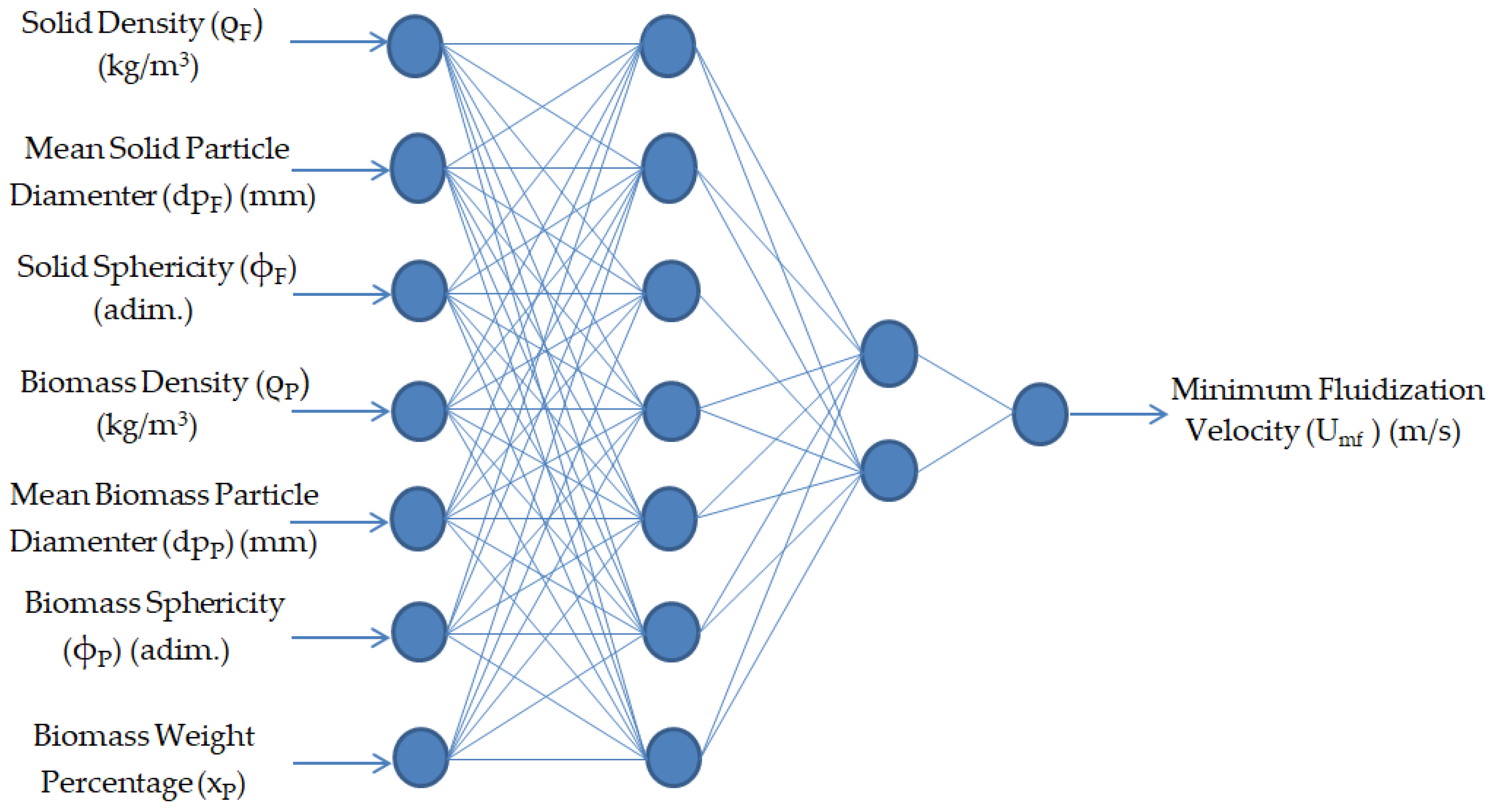
3.1. ANN Models

Two data-based models were developed in order to determine the minimum fluidization velocity of inert-biomass particle mixtures inside a gas–solid fluidized bed using a feed-forward multi-layer perceptron network. This was necessary due to the fact that only a smaller subset of the training data contained sphericity values for both the solid and the biomass inside the FB. Therefore, Model 1 was trained with the full data set (219 sets) and did not contain sphericity as input, and Model 2 was trained only with the subset (114 sets) which contained sphericity values (Figure 1) and, therefore, sphericity was included as an input. The rest of the inputs included densities, particle diameters, and the biomass fraction of the mixture. Both datasets were augmented with information about the minimum fluidization velocity when the biomass fraction was null, that is, regardless of what biomass was entered as input, if the biomass fraction was null, U_mf equaled that of the solid material. Therefore, each model had about 250 datasets in total for training and testing. All datasets are included in the Supplementary Material (Table S1). MATLAB^® Neural Fitting Tool was the software used to develop both ANN models.

Two non-linear activation functions were tried: ReLU and sigmoid. Ultimately, the ReLU was discarded due to poor performance. In addition, the two backpropagation training algorithms were tested, and the Bayesian regularization was chosen instead of the Levenberg–Marquardt which showed worse performance. Both the number of hidden layers and the number of neurons in each one were decided based on a trial and error process. No need was found to apply any other more complex search method for the optimization of those parameters. All the details regarding the ANN models are synthesized in

Table 2. Complete set of Artificial neural networks (ANN) parameters.

Parameter	Model 1 (Without Sphericity)	Model 2
Network Type	Multi-Layer Feed-Forward (MLFF)	Multi-Layer Feed-Forward (MLFF)
Neuron Type	Perceptron	Perceptron
Inputs	5	7
Output	1	1
Normalization Type	Min–Max (−1 to +1)	Min-Max (−1 to +1)
Activation Function	sigmoid (hidden) and linear (output)	sigmoid (hidden) and linear (output)
Training Algorithm	Bayesian Regularization Backpropagation	Bayesian Regularization Backpropagation
Training Sets	252	257
Number of Hidden Layers	2	2
Num. Of Neurons per Layer	7 and 2	7 and 2
Train Ratio	85%	75%
Validation Ratio	N/A	N/A
Test Ratio	15%	25%

.

The procedure to evaluate the ANN’s generalization capability was based on the work of [50]. Once the number of hidden layers (1 or 2 most likely) and the number of neurons in each were established, several candidate networks had to be trained and the best models have to be selected based on their R² value, for instance. Those few best models will be used for simulations with input sets different from those of the training and testing sets in order to assess their generalization capabilities. Among the lot of best R² ANN models, the one having a better generalization may not necessarily be the one showing the best fitting of the training data (higher R²). Additionally, if none of those ANN models has acceptable generalization capacity based on the researcher’s knowledge, retraining the lot may solve the issue. If not, the hyperparameters have to be reset. Both model 1 and model 2 were developed based on the described iterative procedure.

3.2. Data-Based Model Interpretability

Neural networks are black box models in the sense that they are not interpretable. This is because a causal relationship between the inputs and outputs cannot be established. The interpretability of a model is fundamental to the user’s confidence in it, so the user can be able to trust the model’s predictions [51]. In the case presented here, the interpretability of the model will be established with a model-agnostic methodology and a post hoc analysis where, if a certain input is changed and that change modifies the output, then a causal relationship between both exists. A model agnostic analysis involves separating interpretations or explanations and the predictions of the model itself. In other words, it is a model abstraction.

According to [52], a successful causal interpretation must have at least three characteristics: first, a good predictive model; second, some domain or field knowledge; and third, the application of a visualization tool such as the partial dependence plot (PDP [53]). The data-based model’s predictive goodness will be established not only by the experimental or field data fitting performance (training and testing data) and not showing overfit in between but also by its capacity to generalize in the presence of new inputs previously unknown. Moreover, domain knowledge is important for establishing what kind of causal relationships exist between the model’s inputs. These relationships, in particular, might affect the measurement of causal relationships between individual inputs and the output with the PDP.

PDPs show the marginal effect that one or more inputs have over the predicted output of a machine learning model. Generally, the set of inputs of interest is named X_S and the rest of the inputs will be grouped in the set X_C or complement. Then, the PDP of a black box model will estimate the causal effect of X_S on the output Y only if none of the variables on the complementary set X_C is a causal descendant of X_S. Otherwise, there will be no clear causal interpretation obtained with the PDP.

The PDP may be calculated with Equation (35) and consists of averaging all the training and testing sets (n data points) for the inputs in X_C while leaving the inputs in X_S unchanged. Moreover, $\mathrm{g}$ represents the data-based model which, in turn, is an approximation of the real model f, which is not known.

$$\bar{\mathrm{g}}\left({\mathrm{X}}_{\mathrm{S}}\right)=\frac{1}{\mathrm{n}}{\sum }_{\mathrm{i}=1}^{\mathrm{n}}\mathrm{g}({\mathrm{X}}_{\mathrm{S}},{\mathrm{X}}_{\mathrm{C}}^{\mathrm{i}})$$

(35)

3.3. Predictive Correlation

The predictive correlation presented in this work is based on Equation (14), which is the expression also utilized in the work of [32], allowing the inclusion of the biomass fraction. The mean values of density, diameter, and sphericity were determined with Equations (16), (17), and (34), respectively:

$$\mathrm{Ar}=\mathrm{A} \left(1-{\mathrm{x}}_{\mathrm{b}}\right){\bar{\mathsf{\varphi }}}^{\mathrm{C}}{\mathrm{Re}}_{\mathrm{mf}}+\mathrm{B} {\mathrm{x}}_{\mathrm{b}}^{1/2}{\bar{\mathsf{\varphi }}}^{\mathrm{D}}{\mathrm{Re}}_{\mathrm{mf}}^2,$$

(36)

where

$$\mathrm{Ar}=\frac{{\mathsf{\rho }}_{\mathrm{g}}\left(\bar{\mathsf{\rho }}-{\mathsf{\rho }}_{\mathrm{g}}\right)\mathrm{g}{\bar{\mathrm{d}}}^3}{{\mathsf{\mu }}_{\mathrm{g}}^2},$$

(37)

and

$${\mathrm{Re}}_{\mathrm{mf}}=\frac{{\mathsf{\rho }}_{\mathrm{g}}{\mathrm{U}}_{\mathrm{mf} }\bar{\mathrm{d}}}{{\mathsf{\mu }}_{\mathrm{g}}}$$

(38)

The correlation’s parameter optimization was based on the pure random search (PRS) method [54] which is an algorithm that is independent of the gradient of the problem to be maximized or minimized. A total of 112 minimum fluidization values obtained from the literature were used. In this particular case, the goal was to maximize R2. This is based on generating many sets of the parameters A, B, C, and D from a given probability distribution, for example, a normal distribution or, in this particular case, a uniform distribution. Then, every different correlation coefficient set is tested to determine how well it fits the experimental data set.

3.4. Fitting Performance Assessment

As mentioned previously, the coefficient of determination, R², of the predicted and experimental values was the statistical indicator used to show the goodness of fit of the ANN models and the new correlation. R² was calculated with Equation (39).

$${\mathrm{R}}^2=1-\left[\frac{\sum _{\mathrm{i}=1}^{\mathrm{N}}{\left({\mathrm{U}}_{\mathrm{mf} \mathrm{pred},\mathrm{i}}-{\mathrm{U}}_{\mathrm{mf} \exp ,\mathrm{i}}\right)}^2}{{\sum }_{\mathrm{i}=1}^{\mathrm{N}}{\left({\bar{\mathrm{U}}}_{\mathrm{mf} \mathrm{pred}, \mathrm{i}}-{\mathrm{U}}_{\mathrm{mf} \exp ,\mathrm{i}}\right)}^2}\right]$$

(39)

4. Results

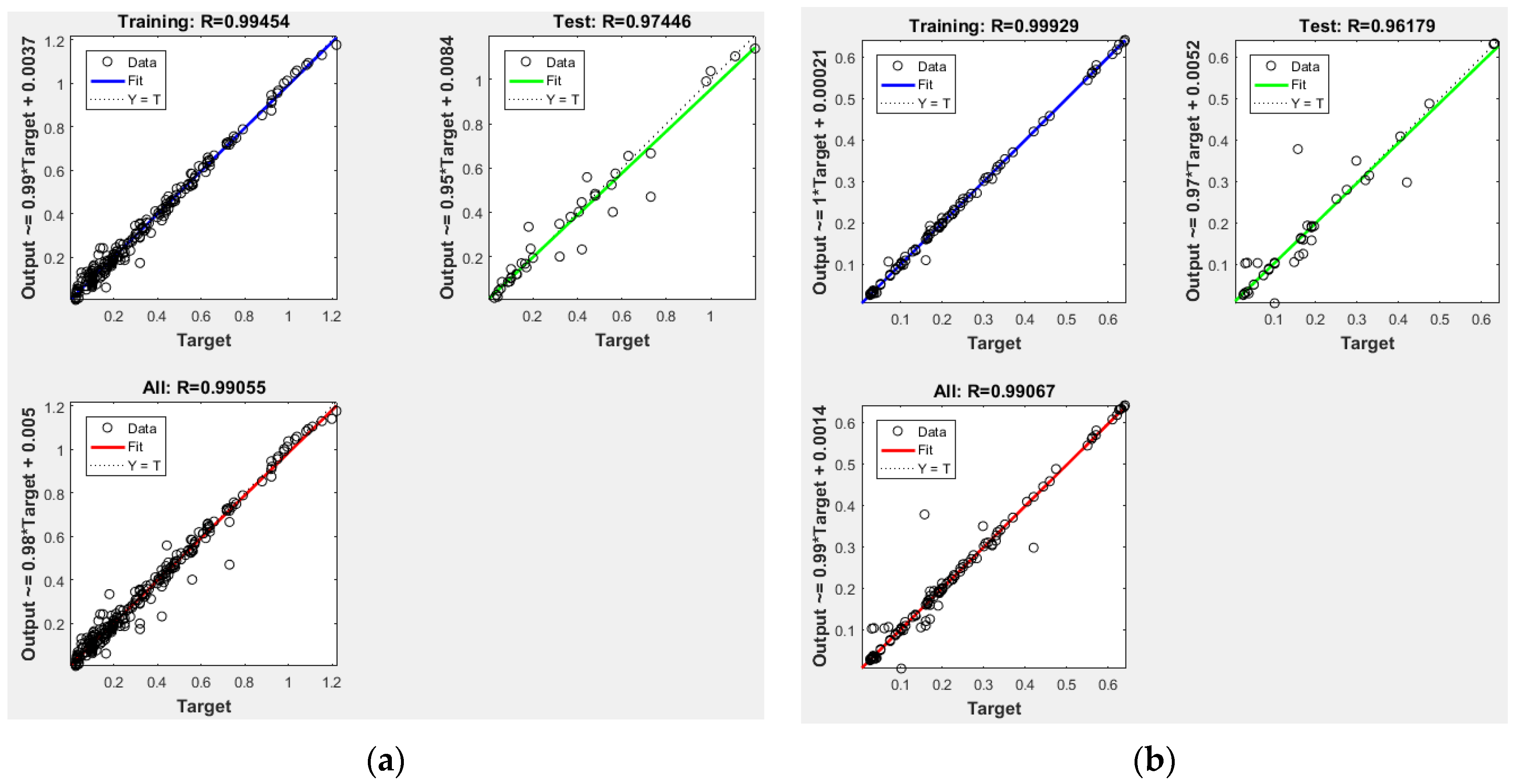
4.1. Models 1 and 2 Training, Testing, and Overall Coefficients of Determination

In this section, the coefficient of determination, R², will be applied in order to assess Models 1 and 2′s fitting performance. The ANN training algorithm randomly divides the complete dataset into two separate subsets: the training set and the testing set. The training set is used for the ANN training process itself (weights and biases) and the testing set is used as a measure of how the ANN is expected to perform in the presence of previously unseen inputs. Generally, the testing set has lower fitting performance when compared to the training set in terms of its coefficient of determination, as can be observed in Figure 2 for both models. Broadly speaking, both models fitted the data well. Moreover, Model 2 had a slightly better fitting performance (0.9906 to 0.9905) when compared to Model 1. Regarding the training set, Model 2 (with more inputs) presented a better fitting performance than Model 1 (0.999 to 0.994).

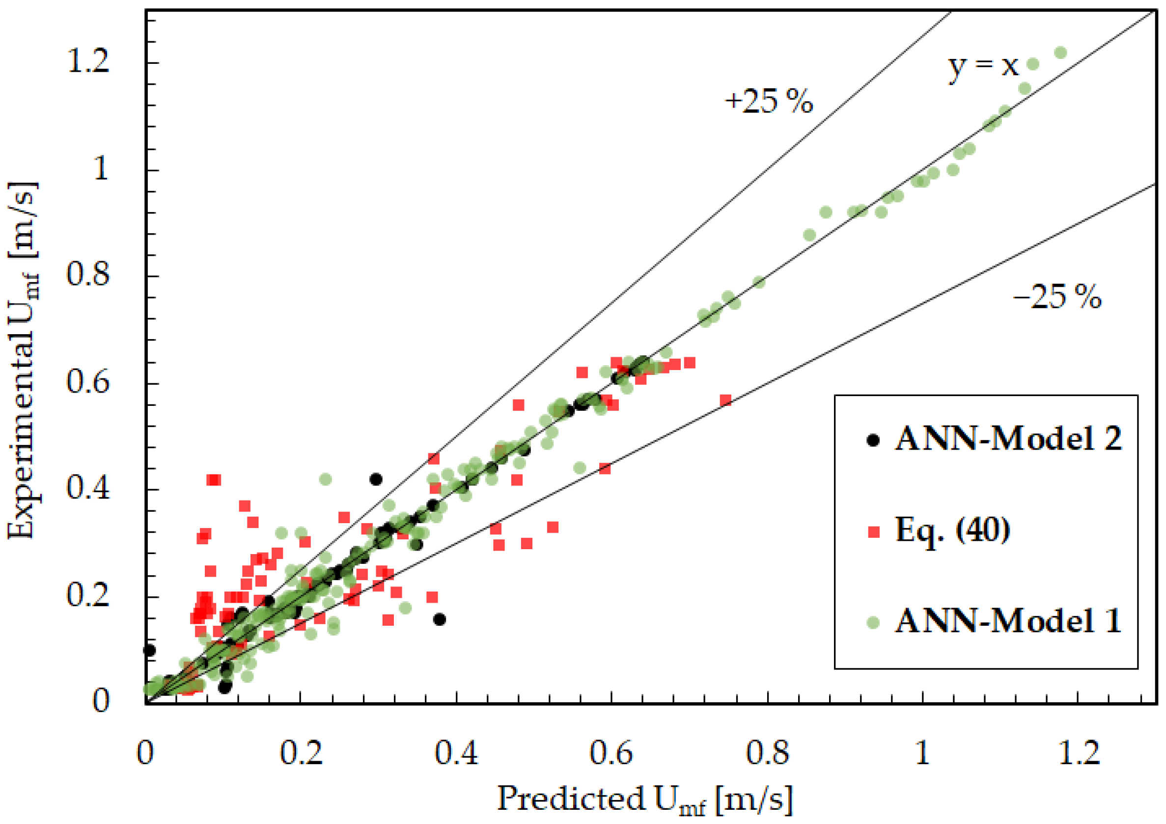
4.2. Accuracy of the ANN-Based Models and Empirical Correlations

The coefficients of Equation (36) were determined as described in Section 3.3, using 112 minimum fluidization velocity data of binary mixtures. From the adjustment, the following correlation was determined:

$$\mathrm{Ar}=1923.384 \left(1-{\mathrm{x}}_{\mathrm{b}}\right){\bar{\mathsf{\varphi }}}^{2.051}{\mathrm{Re}}_{\mathrm{mf}}+24.357 {\mathrm{x}}_{\mathrm{b}}^{1/2}{\bar{\mathsf{\varphi }}}^{0.229}{\mathrm{Re}}_{\mathrm{mf}}^2$$

(40)

Figure 3 shows the experimental values of U_mf compared to the predictions of Equation (40) and ANN models. There are 112 points used in the comparisons using the ANN-Model 2 and 214 points for the ANN-Model 1. It is observed that most of the points of the ANN models are located on the 45° line, so it can be concluded that both models accurately predict the variable of interest. On the other hand, the proposed correlation presents inaccuracies in the prediction of U_mf for low values of the variable. Nevertheless, the prediction improves with errors of less than 25% for higher velocities.

In Figure 4, the results of the predictions were compared with a particular set of U_mf values. In this case, the experimental data was taken from the work of [32], for mixtures of sand (ρ_F = 2450 kg/m³, d_F = 350 μm, ϕ_F = 0.94) and rice husk particles (ρ_P = 635 kg/m³, d_P = 1560 μm, ϕ_P = 0.18). The proposed correlation shows limitations in the accuracy of the U_mf prediction. Regarding the ANN models, ANN-Model 1 accurately reproduces the values of the variable, with an overfit for values of x_b greater than 0.6, and ANN-Model 2 turns out to be accurate for all solid-biomass mixtures.

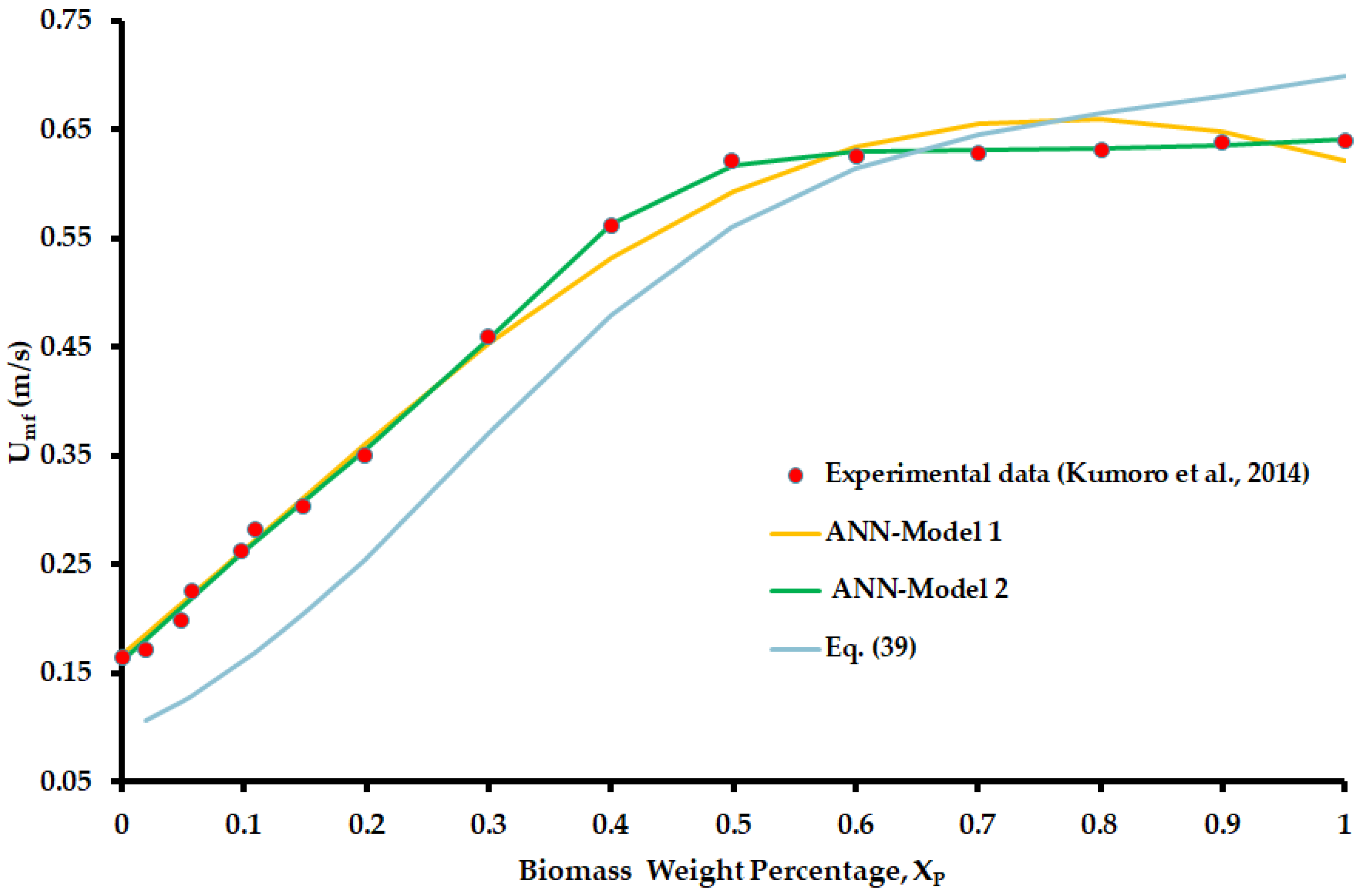
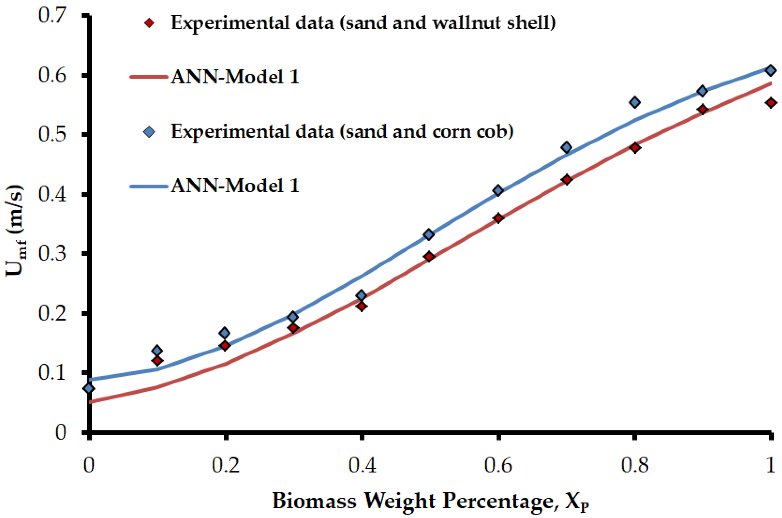
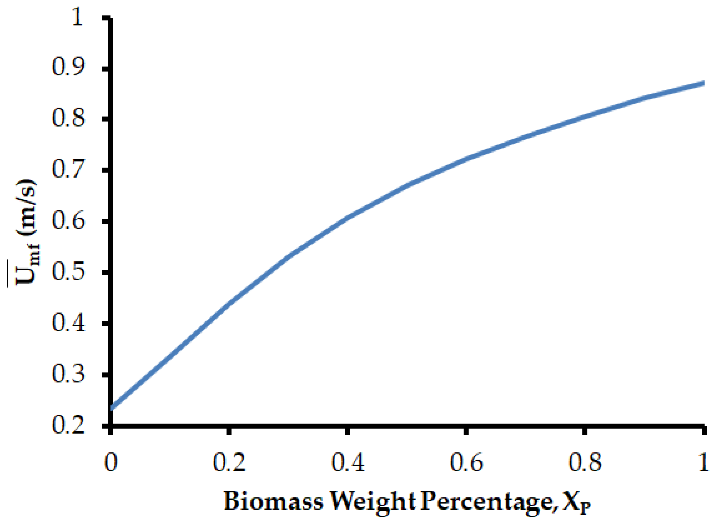
4.3. Effect of the Biomass Fraction on the Minimum Fluidization Velocity U_mf

Simulations were performed with ANN-Model 1 in order to evaluate the effect of the biomass fraction on the minimum fluidization velocity by applying the PDP as a visualization and interpretation tool. In Figure 5, the prediction of U_mf as a function of x_b is presented for the case of [31]. The experimental values are shown in dots and the ANN predictions are shown in continuous lines. As can be seen in Figure 5, there is a direct relationship between U_mf and x_b. This is explained because, in contrast to inert materials, biomass is difficult to fluidize. So, as expected, an increase in the presence of biomass in the binary mixture is followed by an increase in U_mf.

Furthermore, in Figure 6, the PDP confirms the results previously obtained for the Paudel and Feng data [31] by extending it for all data: the average effect of x_b on U_mf is a direct relationship and this is the expected general behavior of the system. The PDP was calculated using Equation (41).

$${\bar{\mathrm{U}}}_{\mathrm{mf}}\left({\mathrm{x}}_{\mathrm{b}}\right)=\frac{1}{\mathrm{n}}{\sum }_{\mathrm{i}=1}^{\mathrm{n}}\mathrm{g}({\mathrm{x}}_{\mathrm{b}},{\mathrm{X}}_{\mathrm{C}}^{\mathrm{i}})$$

(41)

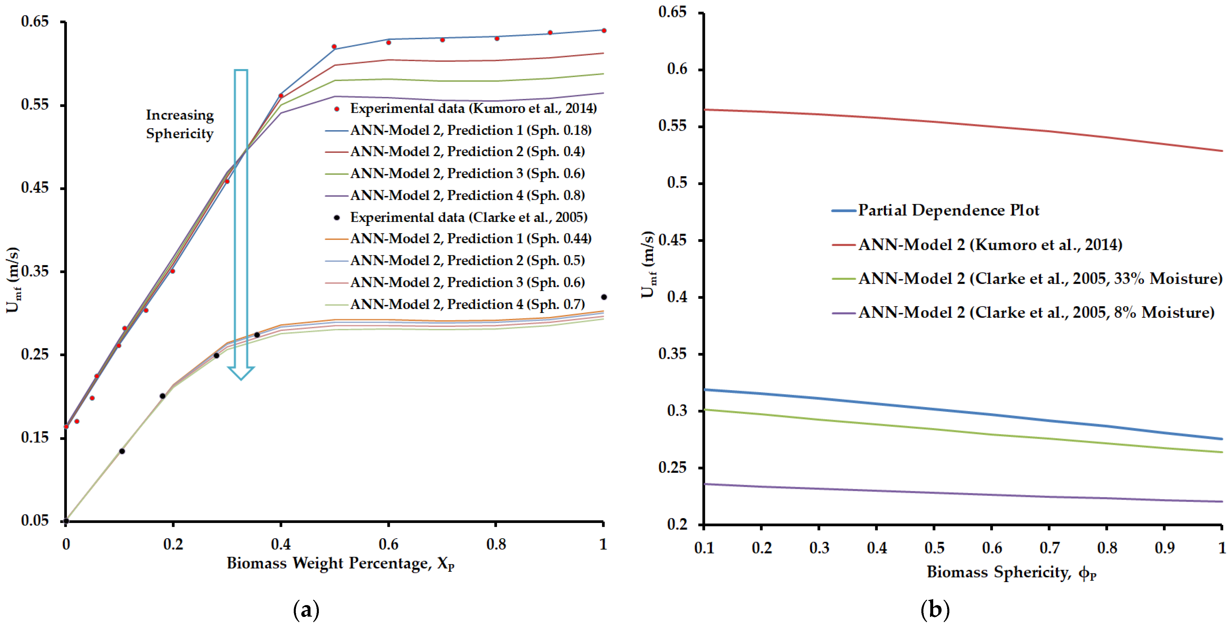
4.4. Effect of Biomass Sphericity on the Minimum Fluidization Velocity

As explained before, ANN-Model 2 incorporates sphericity as an input, so simulations were performed in order to evaluate the effect of the biomass sphericity on the minimum fluidization velocity applying the PDP as a visualization and interpretation tool. In Figure 7a, the prediction of U_mf as a function of x_b is presented for the cases of [32,55]. The last author studied the fluidization of mixtures of glass spheres (ρ_F = 2484 kg/m³, d_F = 322 μm, ϕ_F = 1) and sawdust particles (ρ_P = 433 kg/m³, d_P = 625 μm, ϕ_P = 0.44). The experimental values are shown in dots and the ANN predictions are shown in continuous lines. Several prediction curves are plotted for biomass sphericity values ranging from 0.18 to 0.8 [31] and 0.44 to 0.7 [15]. The results show that U_mf decreases with increasing sphericity. This result is in agreement with the one observed by [29,55]. The last author attributes this behavior to the lower settling velocity of a particle with lower sphericity for solid/Newtonian fluid systems. Additionally, in Figure 7b, the PDP confirms the results obtained previously for the two cases mentioned by extending it for all data: the average effect of sphericity on U_mf is an inverse relationship and this is the expected general behavior of the system. The PDP was calculated using Equation (42).

$${\bar{\mathrm{U}}}_{\mathrm{mf}}\left({\mathrm{x}}_{\mathrm{b}},{\mathsf{\varphi }}_{\mathrm{b}}\right)=\frac{1}{\mathrm{n}}{\sum }_{\mathrm{i}=1}^{\mathrm{n}}\mathrm{g}({\mathrm{x}}_{\mathrm{b}},{\mathsf{\varphi }}_{\mathrm{b}},{\mathrm{X}}_{\mathrm{C}}^{\mathrm{i}})$$

(42)

5. Conclusions

This work is based on the development of three predictive tools for determining the minimum fluidization velocity of biomass and inert particle binary mixtures. In order to do so, an extensive bibliographical survey was conducted and a database of more than 200 datasets was put together. The first predictive model was a correlation based on the biomass fraction, the mean particle diameter, the mean density of the mixture, and the mean particles’ sphericity. Moreover, two ANN models were developed, one considering the particles’ sphericity and another one without this parameter.

In general, both ANN models accurately predict the minimum fluidization velocity of the presented biomass-inert binary mixtures better than the developed correlation, with errors mostly lower than 25%. Specifically, for the data presented in the work of [31], ANN-Model 1 was applied with biomass fraction inputs ranging from 0 to 1. Even though the model follows the tendency well along the domain, fitting performance improved for x_b ≥ 0.5. Similar behavior can be observed for ANN-Model 2.

Additionally, the ANN models allowed predicting U_mf values different from those obtained from the literature by varying, for instance, one or more of the inputs while leaving the rest unchanged. This allowed determining quantitatively how U_mf diminished with an increase in particle sphericity for the cases of [15,32] confirming the observations made by other authors. Then, with the aid of the PDP, these two case-specific results were broadened to the whole domain of data surveyed, thus confirming the trend. Moreover, the PDP was applied to measure the effect of the biomass fraction on U_mf.

In summation, the ANN is a data-based model that can be trained relatively fast, integrating data from many experiments. It is also accurate to fit the training data, allowing us to obtain fast simulations and, together with the PDP, it can be applied to determine the average impact one or more input variables have on the output of the system. On the other hand, due to the limited experimental data available, it is still challenging to develop a model that fits the data well and, at the same time, is able to provide reliable predictions for every possible scenario. Finally, the results of the present work confirm the value of ANN models as low-cost predictive tools for analyzing binary mixture fluidization processes.

References

1. Hilal, N.; Ghannam, M.T.; Anabtawi, M.Z. Effect of bed diameter, distributor and inserts on minimum fluidization velocity. Chem. Eng. Technol. 2001, 24, 161–165. [Google Scholar] [CrossRef]
2. Tang, J.; Chen, X.N.; Lu, C.X.; Zhang, Y.M. Minimum fluidization velocity of binary particles with different Geldart classification. Adv. Mater. Res. 2012, 482, 655–662. [Google Scholar] [CrossRef]
3. Chiba, S.; Chiba, T.; Nienow, A.W.; Kobayashi, H. The minimum fluidisation velocity, bed expansion and pressure-drop profile of binary particle mixtures. Powder Technol. 1979, 22, 255–269. [Google Scholar] [CrossRef]
4. ASTM. Standard Test Method for Measuring the Minimum Fluidization Velocity of Free Flow Powders; ASTM International: Philadelphia, PA, USA, 2012. [Google Scholar]
5. Cáceres-Martínez, L.E.; Guío-Pérez, D.C.; Rincón-Prat, S.L. Significance of the particle physical properties and the Geldart group in the use of correlations for the prediction of minimum fluidization velocity of biomass–sand binary mixtures. Biomass Convers. Biorefin. 2023, 13, 935–951. [Google Scholar] [CrossRef]
6. Soanuch, C.; Korkerd, K.; Piumsomboon, P.; Chalermsinsuwan, B. Minimum fluidization velocities of binary and ternary biomass mixtures with silica sand. Energy Rep. 2020, 6, 67–72. [Google Scholar] [CrossRef]
7. Toschi, F.; Zambon, M.T.; Sandoval, J.; Reyes-Urrutia, A.; Mazza, G.D. Fluidization of forest biomass-sand mixtures: Experimental evaluation of minimum fluidization velocity and CFD modeling. Part. Sci. Technol. 2021, 39, 549–561. [Google Scholar] [CrossRef]
8. Gao, X.; Yu, J.; Li, C.; Panday, R.; Xu, Y.; Li, T.; Ashfaq, H.; Hughes, B.; Rogers, W.A. Comprehensive experimental investigation on biomass-glass beads binary fluidization: A data set for CFD model validation. AIChE J. 2020, 66, e16843. [Google Scholar] [CrossRef]
9. Pérez, N.P.; Pedroso, D.T.; Machin, E.B.; Antunes, J.S.; Ramos, R.A.V.; Silveira, J.L. Fluid dynamic study of mixtures of sugarcane bagasse and sand particles: Minimum fluidization velocity. Biomass Bioenergy 2017, 107, 135–149. [Google Scholar] [CrossRef] [Green Version]
10. Wu, X.; Li, K.; Song, F.; Zhu, X. Fluidization behavior of biomass particles and its improvement in a cold visualized fluidized bed. BioResources 2017, 12, 3546–3559. [Google Scholar] [CrossRef] [Green Version]
11. Pécora, A.A.; Ávila, I.; Lira, C.S.; Cruz, G.; Crnkovic, P.M. Prediction of the combustion process in fluidized bed based on physical–chemical properties of biomass particles and their hydrodynamic behaviors. Fuel Process. Technol. 2014, 124, 188–197. [Google Scholar] [CrossRef]
12. Fotovat, F.; Chaouki, J.; Bergthorson, J. The effect of biomass particles on the gas distribution and dilute phase characteristics of sand–biomass mixtures fluidized in the bubbling regime. Chem. Eng. Sci. 2013, 102, 129–138. [Google Scholar] [CrossRef]
13. Chok, V.S.; Gorin, A.; Chua, H.B. Minimum and complete fluidization velocity for sand-palm shell mixtures, Part I: Fluidization behavior and characteristic velocities. Am. J. Appl. Sci. 2010, 7, 763–772. [Google Scholar] [CrossRef] [Green Version]
14. Gorin, A.; Chok, V.; Wee, S.; Chua, H. Hydrodynamics of binary mixture fluidization in a compartmented fluidized bed. In Proceedings of the 18th International Congress of Chemical and Process Engineering. Chemical Engineering, Chemical Equipment Design and Automation “CHISA”, Prague, Czech Republic, 24–28 August 2008. [Google Scholar]
15. Clarke, K.L.; Pugsley, T.; Hill, G.A. Fluidization of moist sawdust in binary particle systems in a gas–solid fluidized bed. Chem. Eng. Sci. 2005, 60, 6909–6918. [Google Scholar] [CrossRef]
16. Goossens, W.R.A.; Dumont, G.L.; Spaepen, G.L. Fluidization of binary mixtures in the laminar flow region. Chem. Eng. Prog. Symp. Ser. 1971, 67, 38. [Google Scholar]
17. Wen, C.Y.; Yu, Y.-H. Mechanics of fluidization. Chem. Eng. Prog. Symp. Ser. 1966, 62, 100–111. [Google Scholar]
18. Cheung, L.; Nienow, A.W.; Rowe, P.N. Minimum fluidization velocity of a binary mixture of different sized particles. Chem. Eng. Sci. 1974, 29, 1301–1303. [Google Scholar]
19. Rowe, P.N.; Nienow, A.W. Minimum fluidisation velocity of multi-component particle mixtures. Chem. Eng. Sci. 1975, 30, 1365–1369. [Google Scholar] [CrossRef]
20. Hatch, L.P.J. Flow through granular media. Appl. Mech. 1940, 7, 109. [Google Scholar] [CrossRef]
21. Noda, K.; Uchida, S.; Makino, T.; Kamo, H. Minimum fluidization velocity of binary mixture of particles with large size ratio. Powder Technol. 1986, 46, 149–154. [Google Scholar] [CrossRef]
22. Ergun, S. Fluid flow through packed columns. Chem. Eng. Prog. 1952, 48, 89–94. [Google Scholar]
23. Bilbao, R.; Lezaun, J.; Abanades, J.C. Fluidization velocities of sand/straw binary mixtures. Powder Technol. 1987, 52, 1–6. [Google Scholar] [CrossRef]
24. Rao, T.R.; Bheemarasetti, J.R. Minimum fluidization velocities of mixtures of biomass and sands. Energy 2001, 26, 633–644. [Google Scholar] [CrossRef]
25. Kunii, D.; Levenspiel, O. Fluidization Engineering; Butterworth-Heinemann: Oxford, UK, 1991. [Google Scholar]
26. Zhong, W.; Jin, B.; Zhang, Y.; Wang, X.; Xiao, R. Fluidization of biomass particles in a gas−solid fluidized bed. Energy Fuels 2008, 22, 4170–4176. [Google Scholar] [CrossRef]
27. Coltters, R.; Rivas, A.L. Minimum fluidation velocity correlations in particulate systems. Powder Technol. 2004, 147, 34–48. [Google Scholar] [CrossRef]
28. Si, C.; Guo, Q. Fluidization characteristics of binary mixtures of biomass and quartz sand in an acoustic fluidized bed. Ind. Eng. Chem. Res. 2008, 47, 9773–9782. [Google Scholar] [CrossRef]
29. Oliveira, T.J.P.; Cardoso, C.R.; Ataíde, C.H. Bubbling fluidization of biomass and sand binary mixtures: Minimum fluidization velocity and particle segregation. Chem. Eng. Process. Process Intensif. 2013, 72, 113–121. [Google Scholar] [CrossRef]
30. Shao, Y.; Ren, B.; Jin, B.; Zhong, W.; Hu, H.; Chen, X.; Sha, C. Experimental flow behaviors of irregular particles with silica sand in solid waste fluidized bed. Powder Technol. 2013, 234, 67–75. [Google Scholar] [CrossRef]
31. Paudel, B.; Feng, Z.G. Prediction of minimum fluidization velocity for binary mixtures of biomass and inert particles. Powder Technol. 2013, 237, 134–140. [Google Scholar] [CrossRef]
32. Kumoro, A.; Nasution, D.; Cifriadi, A.; Purbasari, A.; Falaah, A. A new correlation for the prediction of minimum fluidization of sand and irregularly shape biomass mixtures in a bubbling fluidized bed. Int. J. Appl. Eng. Res. 2014, 9, 21561–21573. [Google Scholar]
33. Jena, H.M.; Roy, G.K.; Biswal, K.C. Studies on pressure drop and minimum fluidization velocity of gas–solid fluidization of homogeneous well-mixed ternary mixtures in un-promoted and promoted square bed. J. Chem. Eng. 2008, 145, 16–24. [Google Scholar] [CrossRef]
34. Reyes-Urrutia, A.; Soria, J.; Saffe, A.; Zambon, M.; Echegaray, M.; Suárez, S.G.; Rodriguez, R.; Mazza, G. Fluidization of biomass: A correlation to assess the minimum fluidization velocity considering the influence of the sphericity factor. Part. Sci. Technol. 2021, 39, 1020–1040. [Google Scholar] [CrossRef]
35. Brunton, S.L.; Noack, B.R.; Koumoutsakos, P. Machine learning for fluid mechanics. Annu. Rev. Fluid Mech. 2020, 52, 477–508. [Google Scholar] [CrossRef] [Green Version]
36. Hornik, K.; Stinchcombe, M.; White, H. Multilayer feedforward networks are universal approximators. Neural Netw. 1989, 2, 359–366. [Google Scholar] [CrossRef]
37. Pinkus, A. Approximation theory of the MLP model in neural networks. Acta Numer. 1999, 8, 143–195. [Google Scholar] [CrossRef]
38. Hoskins, J.C.; Himmelblau, D.M. Artificial neural network models of knowledge representation in chemical engineering. Comput. Chem. Eng. 1988, 12, 881–890. [Google Scholar] [CrossRef]
39. Himmelblau, D.M. Applications of artificial neural networks in chemical engineering. Korean J. Chem. Eng. 2000, 17, 373–392. [Google Scholar] [CrossRef]
40. Pirdashti, M.; Curteanu, S.; Kamangar, M.H.; Hassim, M.H.; Khatami, M.A. Artificial neural networks: Applications in chemical engineering. Rev. Chem. Eng. 2013, 29, 205–239. [Google Scholar] [CrossRef]
41. Andrejević Stošović, M.; Litovski, V. Applications of artificial neural networks in electronics. Electronics 2017, 21, 87–94. [Google Scholar] [CrossRef]
42. Larachi, F.; Iliuta, I.; Rival, O.; Grandjean, B.P. Prediction of minimum fluidization velocity in three-phase fluidized-bed reactors. Ind. Eng. Chem. Res. 2000, 39, 563–572. [Google Scholar] [CrossRef]
43. Zhong, W.; Chen, X.; Grace, J.R.; Epstein, N.; Jin, B. Intelligent prediction of minimum spouting velocity of spouted bed by back propagation neural network. Powder Technol. 2013, 247, 197–203. [Google Scholar] [CrossRef]
44. Maiti, S.B.; Let, S.; Bar, N.; and Das, S.K. Non-spherical solid-non-Newtonian liquid fluidization and ANN modelling: Minimum fluidization velocity. Chem. Eng. Sci. 2018, 176, 233–241. [Google Scholar] [CrossRef]
45. Karimi, M.; Vaferi, B.; Hosseini, S.H.; Rasteh, M. Designing an efficient artificial intelligent approach for estimation of hydrodynamic characteristics of tapered fluidized bed from its design and operating parameters. Ind. Eng. Chem. Res. 2018, 57, 259–267. [Google Scholar] [CrossRef]
46. Rasteh, M.; Farhadi, F.; Bahramian, A. Hydrodynamic characteristics of gas–solid tapered fluidized beds: Experimental studies and empirical models. Powder Technol. 2015, 283, 355–367. [Google Scholar] [CrossRef]
47. Hosseini, S.H.; Valizadeh, M.; Olazar, M.; Altzibar, H. Minimum spouting velocity of draft tube conical spouted beds using the neural network approach. Chem. Eng. Technol. 2017, 40, 1132–1139. [Google Scholar] [CrossRef]
48. Hosseini, S.H.; Rezaei, M.J.; Bag-Mohammadi, M.; Altzibar, H.; Olazar, M. Smart models to predict the minimum spouting velocity of conical spouted beds with non-porous draft tube. Chem. Eng. Res. Des. 2018, 138, 331–340. [Google Scholar] [CrossRef]
49. Targino, T.G.; Freire, J.T.; Perazzini, M.T.B.; Perazzini, H. Fluidization design parameters of agroindustrial residues for biomass applications: Experimental, theoretical, and neural networks approach. Biomass Convers. Biorefin. 2021, 13, 4213–4228. [Google Scholar] [CrossRef]
50. Fabani, M.P.; Capossio, J.P.; Román, M.C.; Zhu, W.; Rodriguez, R.; Mazza, G. Producing non-traditional flour from watermelon rind pomace: Artificial neural network (ANN) modeling of the drying process. J. Environ. Manag. 2021, 281, 111915. [Google Scholar] [CrossRef] [PubMed]
51. Ribeiro, M.T.; Singh, S.; Guestrin, C. Model-agnostic interpretability of machine learning. arXiv 2016, arXiv:1606.05386. [Google Scholar]
52. Zhao, Q.; Hastie, T. Causal interpretations of black-box models. J. Bus. Econ. Stat. 2021, 39, 272–281. [Google Scholar] [CrossRef]
53. Friedman, J.H. Greedy function approximation: A gradient boosting machine. Ann. Stat. 2001, 29, 1189–1232. [Google Scholar] [CrossRef]
54. Zabinsky, Z.B. Pure random search and pure adaptive search. In Stochastic Adaptive Search for Global Optimization; Springer: Boston, MA, USA, 2003; pp. 25–54. [Google Scholar]
55. Let, S.; Bar, N.; Basu, R.K.; Das, S.K. Minimum Fluidization Velocities of Binary Solid Mixtures: Empirical Correlation and Genetic Algorithm-Artificial Neural Network Modeling. Chem. Eng. Technol. 2022, 45, 73–82. [Google Scholar] [CrossRef]
Figure 1. ANN-Model 2 (bias inputs are omitted from the figure for clarity). Model 1 has the same architecture but without the two sphericities as inputs.
Fluids 08 00128 g001
Figure 2. (a) Model 1 training and testing results; (b) Model 2 training and testing results (both from MATLAB® Neural Fitting Tool).
Fluids 08 00128 g002
Figure 3. Comparison among experimental and predicted values of Umf to the mixtures.
Fluids 08 00128 g003
Figure 4. Prediction vs. experimental values of Umf for mixtures of sand-rice husk particles. Experimental data extracted from [32].
Fluids 08 00128 g004
Figure 5. Simulations using ANN-Model 1 for the experimental data of case [31]. Match between experimental data and model’s predictions. ρF = 2630 kg/m3, dF = 240 μm (sand), ρP =1200 kg/m3, dP = 856 μm (walnut shell), ρP =1080 kg/m3, dP = 1040 μm (corn cob).
Fluids 08 00128 g005
Figure 6. Simulations using Model 1. Average effect of biomass fraction calculated with the PDP.
Fluids 08 00128 g006
Figure 7. Simulations using Model 2 varying the sphericity values: (a) Cases of [15,32]; (b) average effect of sphericity calculated with the PDP (xb = 0.4).
Fluids 08 00128 g007