Laboratory Models of Planetary Core-Style Convective Turbulence

Abstract

The connection between the heat transfer and characteristic flow velocities of planetary core-style convection remains poorly understood. To address this, we present novel laboratory models of rotating Rayleigh–Bénard convection in which heat and momentum transfer are simultaneously measured. Using water (Prandtl number, $Pr\simeq 6$) and cylindrical containers of diameter-to-height aspect ratios of $\Gamma \simeq 3,1.5,0.75$, the non-dimensional rotation period (Ekman number, E) is varied between ${10}^{-7}\lesssim E\lesssim 3\times {10}^{-5}$ and the non-dimensional convective forcing (Rayleigh number, $Ra$) ranges from ${10}^7\lesssim Ra\lesssim {10}^{12}$. Our heat transfer data agree with those of previous studies and are largely controlled by boundary layer dynamics. We utilize laser Doppler velocimetry (LDV) to obtain experimental point measurements of bulk axial velocities, resulting in estimates of the non-dimensional momentum transfer (Reynolds number, $Re$) with values between $4\times {10}^2\lesssim Re\lesssim 5\times {10}^4$. Behavioral transitions in the velocity data do not exist where transitions in heat transfer behaviors occur, indicating that bulk dynamics are not controlled by the boundary layers of the system. Instead, the LDV data agree well with the diffusion-free Coriolis–Inertia–Archimedian (CIA) scaling over the range of $Ra$ explored. Furthermore, the CIA scaling approximately co-scales with the Viscous–Archimedian–Coriolis (VAC) scaling over the parameter space studied. We explain this observation by demonstrating that the VAC and CIA relations will co-scale when the local Reynolds number in the fluid bulk is of order unity. We conclude that in our experiments and similar laboratory and numerical investigations with $E\gtrsim {10}^{-7}$, $Ra\lesssim {10}^{12}$, $Pr\simeq 7$, heat transfer is controlled by boundary layer physics while quasi-geostrophically turbulent dynamics relevant to core flows robustly exist in the fluid bulk.

1. Introduction

The rotating convective turbulence of electrically conducting liquid metal layers within planets is responsible for the generation of their global-scale magnetic fields [1,2]. The details of core-style turbulence, particularly the connection between heat and momentum transfer, remain elusive. These turbulent flows that exist at planetary conditions and are remote from direct measurement are difficult to directly model due to their complex and extreme nature. Laboratory experiments, direct numerical simulations (DNS), and theoretical models use various simplified approaches to understand the turbulent fluid physics of dynamo-generating mechanisms (e.g., [3,4,5]). The goal of these reduced models is to develop accurate scaling laws characterizing fundamental system behaviors that can be extrapolated to the extreme settings at which planetary dynamos exist.

One of the most common models used to study this problem is that of rotating Rayleigh–Bénard convection (RRBC), where a layer of fluid is heated from below while simultaneously cooled from above and rotated about a vertical axis. The laboratory experiments in this RRBC study implement a right cylindrical geometry, thus removing any effects of spherical curvature. A number of recent studies have focused on characterizing the effects of cylindrical sidewalls on rotating heat transfer (e.g., [6,7,8,9,10,11,12]). These studies show that sidewall effects are most pronounced very close to the onset of convection. Overall, bulk cylindrical laboratory heat transfer data agree with those of unconfined periodic DNS. Furthermore, the recent study by Gastine and Aurnou [13] directly compares the heat transfer of the spherical shell DNS to that of the local Cartesian DNS and concludes that local, non-spherical models can be used to understand spherical systems (see also Wang et al. [14]). The results of these recent studies demonstrate that laboratory cylinders are a useful and relevant tool for studying spherical shell-core dynamics.

To illustrate our model system, Figure 1 displays a schematic of the northern hemisphere of Earth’s core region. The cylinder located at a high latitude and aligned with the rotation axis represents one of the laboratory containers used in this work. Our experiments simulate a local, polar parcel of planetary core fluid convecting under the influence of axial rotation and buoyancy forcing. The interior of the cylinder is filled with an illustrative subset of the visualization of a geostrophically turbulent laboratory experiment. The bottom (top) boundaries of the cell are red (blue) to represent the warm (cold) fluid in parallel with the warmer/red inner core boundary (cooler/blue core–mantle boundary).

The outer core region in Figure 1 shows a meridional slice of the instantaneous radial velocity of a dynamo simulation adapted from Sheyko et al. [15]. From this meridional slice, we see that fluid motions are largely aligned with the rotation axis. Furthermore, these fluid motions, which are generated in the presence of a magnetic field and a spherical shell geometry, compare qualitatively to the visualization of the purely hydrodynamic cylindrical laboratory experiment shown in Figure 1. Thus, Figure 1 highlights the ability to compare a hydrodynamic laboratory experiment with a cylindrical geometry to a spherical shell DNS model that uses a magnetohydrodynamic description.

Numerous studies have found that the stabilizing effect of rotation on turbulent convection acts to vertically align motion in the fluid bulk along the rotation axis, regardless of geometry [16,17,18,19,20,21,22,23,24,25,26]. In addition, many dynamo studies have also found that the large-scale dynamics of core-style flows are largely governed, at leading order, by the non-magnetic dynamics of rapidly rotating, so-called quasi-geostrophic turbulence [27,28,29,30,31,32,33,34,35,36,37]. These results motivate further exploration of rotating convective turbulence, which is carried out in this work. Thus, the use of a purely hydrodynamic fluid (water) in this study can be used to explore relevant non-magnetic quasi-geostrophic turbulent dynamics.

Heat transfer is the most common diagnostic used to characterize convective dynamics in studies of RRBC (e.g., [37,38,39,40,41,42,43,44,45]). RRBC studies typically assume that global heat transfer will agree with and correspond to bulk velocity dynamics. Furthermore, many studies have found that convective heat transport is controlled by the dynamics occurring in the boundary layers of the system (cf. [21,37,46,47]). Contrastingly, the theory for the dynamics of the quasi-geostrophic turbulence thought to exist in planetary dynamo systems is independent of boundary physics and system diffusivities [48,49,50,51,52,53]. Thus, it remains unclear as to whether or not flow regimes indicated by the study of heat transfer alone are indeed representative of the bulk dynamical behavior of convection systems. Therefore, simultaneous measurements of heat transfer and bulk system velocities are needed.

The experiments in this study display heat transfer that is controlled by the boundary layer physics, while bulk velocities follow a diffusion-free scaling related to a balance between the Coriolis force, inertia, and buoyancy in the system (cf. [25,53,54,55]). We show this by simultaneously measuring convective velocities and heat transfer and directly comparing these measurements to results from DNS. As the velocity data appear to robustly follow a diffusion-free scaling, our results indicate that quasi-geostrophic bulk turbulence is reached even when heat transfer still depends on diffusive processes occurring in the boundary layers.

In Section 2, we detail the system parameters and scaling behaviors relevant to this work. In Section 3, we describe our experimental and numerical methods. The non-rotating convection results are described in Section 4.1 and the rotating convection results are presented in Section 4.2. The co-scaling of the two velocity predictions in this study, the Viscous–Archimedian–Coriolis (VAC) and Coriolis–Inertia–Archimedian (CIA) scalings, is discussed in Section 4.2.1. An analysis of local flow estimates and their comparison to asymptotic theory is provided in Section 4.2.2. Lastly, a discussion of this work and its implications for planetary dynamo systems is given in Section 5.

2. System Parameters and Scaling Behaviors

2.1. Rayleigh–Bénard Convection (RBC)

2.1.1. System Parameters

The consideration of non-rotating Rayleigh–Bénard convection (RBC) is an important precursor for the study of analogous rotating systems. The control parameters for an RBC system are the dimensionless Rayleigh and Prandtl numbers. The Rayleigh number, $Ra$, describes the ratio of thermal buoyancy to viscous and thermal diffusion and is given as:

$$Ra=\frac{\mathrm{thermal}\mathrm{buoyancy}}{\mathrm{thermal} \& \mathrm{viscous} \mathrm{diffusion}}=\frac{\alpha g\Delta T{H}^3}{\nu \kappa },$$

(1)

where $\alpha$ (1/K) is the thermal expansivity of the fluid, g (m/s${}^2$) is the gravitational acceleration, $\Delta T$ (K) is the temperature difference across the fluid layer, H (m) is the height of the fluid layer, $\nu$ (m${}^2$/s) is the kinematic viscosity of the fluid, and $\kappa$ (m${}^2$/s) is the thermal diffusivity of the fluid. The Prandtl number, $Pr$, is the ratio between viscous and thermal diffusion and is given as:

$$Pr=\frac{\mathrm{viscous}\mathrm{diffusion}}{\mathrm{thermal}\mathrm{diffusion}}=\frac{\nu }{\kappa }.$$

(2)

Lastly, $\Gamma$ is the aspect ratio of the cylindrical container:

$$\Gamma =\frac{D}{H},$$

(3)

where $D=2R$ is the diameter of the fluid layer.

2.1.2. RBC Heat Transfer Scaling Behavior

In RBC, the non-dimensional heat transfer is described by the Nusselt number, $Nu$, which is the ratio of the total heat flux through the system relative to the conductive heat flux in the absence of convection:

$$Nu=\frac{\mathrm{total}\mathrm{heat}\mathrm{flux}}{\mathrm{conductive}\mathrm{heat}\mathrm{flux}}=\frac{qH}{k\Delta T},$$

(4)

where q (W/m${}^2$) is the total heat flux through the system and k (W/mK) is the thermal conductivity of the fluid. The Nusselt number describes the efficiency of global heat transport, and trends in the Nusselt number are related to fundamental convective behaviors (e.g., [35,56,57,58,59]).

In $Pr\sim \mathcal{O}\left(1\right)$ RBC systems that are far past convective onset, a scaling relationship between $Nu$ and the input parameter $Ra$ exists of the form:

$$Nu=cR{a}^{\alpha },$$

(5)

where c is the pre-factor and $\alpha$ is the scaling exponent. Over the accessible range of parameter space covered to date by $Pr\sim \mathcal{O}\left(1\right)$ laboratory experiments and DNS (i.e., ${10}^3\lesssim Ra\lesssim {10}^{15}$), the scaling exponent, $\alpha$, in (5) is found to vary between $\alpha \simeq 2/7$ and $\alpha \simeq 1/3$ [38,40,60,61,62,63,64,65,66]. The $\alpha \simeq 1/3$ scaling relation arises when the fluid bulk becomes approximately isothermal and the boundary layers do not interact due to vigorous bulk convective mixing [45,67,68,69,70,71,72,73,74]. We illustrate the RBC heat transfer behavior we test in this study in Figure 2a, where the partially faded fuchsia line, $N{u}_0^{*}$, corresponds to the empirical best fit of the experimental data in Cheng et al. [45], with a pre-factor of $c=0.11$ and an exponent of $\alpha =0.308$.

2.1.3. RBC Momentum Transfer Scaling Behavior

The Reynolds number, $Re$, describes the momentum transfer in RBC systems and is the ratio of inertial advection to viscous diffusion, which is given as:

$$Re=\frac{\mathrm{inertial}\mathrm{advection}}{\mathrm{viscous}\mathrm{diffusion}}=\frac{uH}{\nu },$$

(6)

where u (m/s) is a characteristic system velocity. Using a free-fall velocity, $u_{\mathrm{ff}}\sim \sqrt{\alpha g\Delta TH}$, to estimate the system scale velocity, u, in (6), a relationship between $Re$ and $Ra$ exists of the form:

$$Re=bR{a}^{\gamma }\sim R{a}^{1/2}$$

(7)

when $Pr\sim \mathcal{O}\left(1\right)$ [56,63,78,79,80]. A best fit exponent of $\gamma \simeq 0.45$ has been found experimentally by Qiu and Tong [77]. The faded black line in Figure 2b shows $Re$ as a function of $Ra$ according to (7), with the best fitfit pre-factor, $b=0.102$, and exponent, $\gamma =0.447$, from [77]. This line serves as an upper-bounding estimate of the RRBC momentum transfer discussed in Section 2.2.3 below.

2.2. Rotating Convection (RRBC)

2.2.1. System Parameters

Two new non-dimensional control parameters are introduced to an RBC system with rotation: the Ekman number, E, and the Froude number, $Fr$. The Ekman number describes the ratio of viscous diffusion to the Coriolis force and is given as:

$$E=\frac{\mathrm{viscous}\mathrm{diffusion}}{\mathrm{Coriolis}}=\frac{\nu }{2\Omega H^2},$$

(8)

where $\Omega$ (rad/s) is the angular rotation rate of the container. The Froude number characterizes the ratio of centrifugal buoyancy to gravitational buoyancy in the system and is given as:

$$Fr=\frac{\mathrm{centrifugal}\mathrm{buoyancy}}{\mathrm{gravitational}\mathrm{buoyancy}}=\frac{{\Omega }^{2}R}{g},$$

(9)

where R (m) is the radius of the cylindrical container.

Centrifugal buoyancy is argued to play a weak role in planetary core convection as estimates of the Froude number remain small, i.e., $Fr\lesssim {10}^{-2}$, in planetary dynamo systems. Thus, the DNS herein do not include centrifugal buoyancy effects. However, in our laboratory experiments, centrifugal buoyancy cannot be removed. According to Horn and Aurnou [81], heat transfer measurements are not significantly altered by centrifugal buoyancy until $Fr\gtrsim \Gamma /2$, i.e., when the Froude number exceeds half the aspect ratio of the container used. This constraint is only exceeded in our most extreme dataset, where $E\simeq 1.27\times {10}^{-7}$ and $\Gamma \simeq 0.74$. The potential effect of the large centrifugal buoyancy force in this dataset is discussed in Section 4.2.

2.2.2. RRBC Heat Transfer Scaling Behavior

In a geometrically confined RRBC water system, convection will first onset in the form of wall modes [82,83,84,85]. The criterion for the onset of wall modes in low E RRBC under the assumption that the curvature of a confining cylinder can be neglected is given in Zhang and Liao [75] as:

$$R{a}_C^W\simeq 31.8E^{-1}.$$

(10)

For $Pr>0.68$, steady, bulk-filling convection is predicted to occur in a horizontally infinite plane layer in the limit of small E when: [76]

$$R{a}_C^S\simeq 8.7E^{-4/3}.$$

(11)

After the onset of steady RRBC, different distinguishable scaling trends in heat transfer behavior have been observed and have been reviewed in Cheng et al. [3], Plumley and Julien [58], Kunnen [17], and Ecke and Shishkina [16].

Several recent studies have characterized the effects of lateral boundaries on rotating heat transfer [6,7,8,11,12,16,86,87,88]. In de Wit et al. [9] and Lu et al. [10], the ‘sidewall circulation’ in which enhanced heat transport occurs near container sidewalls is quantified. These studies also show that the bulk heat transfer in confined experiments is in good agreement with that of unconfined periodic DNS. The experiments herein do not have temperature sensors in locations that enable the quantification of heat transfer near container sidewalls. Nonetheless, in Section 4.2, we show that the measured heat transport data of the experiments in this work, which exist at least three times past steady onset, are in good agreement with those of laterally unconfined DNS.

Neglecting sidewall effects, a scaling relation for the heat transfer occurring in the regime past steady onset, where the entire fluid layer (i.e., the bulk and boundary layers) is thought to be rotationally constrained, can be expressed in terms of the criticality past steady onset as:

$$N{u}_{\Omega }\sim {(Ra/R{a}_C^S)}^{\beta }$$

(12)

(e.g., [58]). As the Ekman number decreases, $\beta$ steepens due to Ekman pumping effects, which boost the heat transfer [47,89,90]. Cheng et al. [3] estimate that the scaling exponent $\beta$ in the rotationally constrained heat transfer regime depends on the Ekman number as: (cf. [10])

$$\beta =-0.45-0.59lo{g}_{10}\left(E\right).$$

(13)

The regime described by (12) is often referred to as the ‘columnar’ or ‘convective Taylor column’ regime, although we note that the direct connection between (12) and the existence of convective columns throughout this regime remains unclear (cf. [45,47,91]). Nonetheless, it is presently thought that convection in this regime occurs in the form of long, thin columns aligned with the axis of rotation when $Ra/R{a}_C^S\gtrsim 2$ (e.g., [18,82,92,93,94,95,96]). The cross-axial width of a steady RRBC column that develops at onset is: [76,97,98,99,100,101,102]

$${\ell }_{\mathrm{crit}}\simeq 2.4E^{1/3}H.$$

(14)

Far past the onset of convection in RRBC, heat transfer behaves as if it is non-rotating according to (5) (e.g., [8,10,22,41,45,59,64,65,103]). The boundary layer physics involved in the transition of the RRBC heat transfer from being buoyancy dominated to rotationally constrained is complex, as elucidated in Julien et al. [89]. This boundary layer physics is not the focus of this study and, furthermore, we do not have temperature sensors in locations that enable us to resolve this physics. Nonetheless, we expect that the dominant boundary layer when RRBC heat transfer is buoyancy controlled can be estimated as the non-rotating thermal boundary layer:

$${\delta }_T^{\mathrm{NR}}\sim H/\left(2Nu\right),$$

(15)

where ${\delta }_T^{\mathrm{NR}}$ (m) is the thickness of a single RBC thermal boundary layer [46,50,89].

RRBC heat transfer gradually becomes more and more rotationally constrained when lowering the convective supercriticality, and eventually, the viscous Ekman boundary layer becomes the dominant boundary layer, estimated here as: [64,97]

$${\delta }_E\sim 3E^{1/2}H.$$

(16)

Thus, we predict that non-rotating-style heat transfer in RRBC will occur when the RBC thermal boundary layer becomes thinner than the Ekman boundary layer, i.e., when:

$${\delta }_E/{\delta }_T^{\mathrm{NR}}>1.$$

(17)

Numerous convection studies with a variety of applications have found that heat transport is controlled by the dominance of the relevant boundary layers. While the details of boundary layer influence on heat transport vary, such applications include convection studies with non-uniform heating (e.g., [104,105,106,107,108,109,110,111,112]); studies with non-uniform boundaries [113,114,115,116,117,118,119,120,121]; and studies of rotating convection with libration, precession, or tidal deformation (e.g., [122,123,124,125,126,127]), among others.

Empirically, a ‘transition’ Rayleigh number, $R{a}_T$, can be defined in an attempt to characterize the transition from non-rotating-style heat transfer to a rotationally constrained fluid layer. The empirical intersection of these two heat transfer scalings, (5) and (12), respectively, define $R{a}_T$ as: [65]

$$R{a}_T=c^{1/(\beta -\alpha )}{\left(R{a}_C^S\right)}^{\beta /(\beta -\alpha )}=8.7^{\beta /(\beta -\alpha )}{c}^{1/(\beta -\alpha )}{E}^{4\alpha /3(\alpha -\beta )}.$$

(18)

Previous studies (e.g., [10,22,46,50,64,65,128,129]) find that the transition from non-rotating style heat transfer to the rotationally dominated heat transfer regime occurs over a gradual region that is not well described by (18). A number of different ideas exist regarding this gradual transition region (cf. [3,10,17]).

We choose to implement (18) in order to create a simple, testable framework for RRBC heat transfer behavior. Our framework does not incorporate recent findings surrounding wall mode heat transfer occurring near convective onset (i.e., [10]). Figure 2a is a ‘strawman’ that shows this framework by displaying $Nu$ vs. $Ra$ for an RRBC system with fixed $E={10}^{-6}$, $Pr\simeq 6$. The onset of wall mode convection given by (10) is denoted by an open star and the onset of steady convection given by (11) is denoted by a solid star. After steady onset, the heat transfer efficiency, $Nu$, scales steeply with increases in $Ra$, as given by (12) (blue line). Past $R{a}_T$, given by (18) (dashed line), the heat transfer behaves as though the system is not rotating according to (5) (fuchsia line).

2.2.3. RRBC Momentum Transfer Scaling Behavior

The balance between buoyant energy production and dissipation in convection systems results in an exact relation between velocity and heat transfer. This holds for both RBC [62,130,131] and RRBC systems [25,55,132,133,134,135]. In RRBC, the use of this relation results in the generalized non-dimensional velocity scaling:

$$Re\sim {\left[\frac{Ra(Nu-1)}{P{r}^2}E\left(\frac{H}{\ell }\right)\right]}^{\frac{1}{2}},$$

(19)

where ℓ (m) is the characteristic cross-axial length scale of convection. The term $Ra(Nu-1)/P{r}^2$ in (19) is the non-dimensional buoyancy flux (e.g., [134]). Thus, a non-dimensional velocity scaling in RRBC depends on: (1) the flux of buoyant energy; (2) the rotation period (via E); and (3) the anisotropy of the flow field, $\ell /H$.

Two theoretical length scales describing ℓ exist in RRBC. The first is derived from linear theory [76] and describes the width of RRBC columns as given by (14):

$${\ell }_{\mathrm{crit}}/H\sim E^{1/3}.$$

(20)

Substituting (20) into (19), we recover:

$$R{e}_{\mathrm{VAC}}\sim {\left(\frac{Ra(Nu-1)}{P{r}^2}\right)}^{\frac{1}{2}}{E}^{\frac{1}{3}}.$$

(21)

Equation (21) is referred to as a ‘VAC’ scaling due to the underlying assumption that a triple balance exists between the Viscous–Archimedean (buoyancy)–Coriolis forces at steady onset [22,24,27,55,134,136].

The second length scale in RRBC provides a different scaling of $Re$ than that of (21). Inertial theory predicts that: [54,137]

$${\ell }_{\mathrm{turb}}/H\sim R{o}^{1/2},$$

(22)

where $Ro=ReE$ is the Rossby number. $Ro$ describes the ratio of inertial advection to the Coriolis force:

$$Ro=\frac{u}{2\Omega H}.$$

(23)

The substitution of (22) into (19) yields:

$$R{e}_{\mathrm{CIA}}\sim {\left(\frac{Ra(Nu-1)}{P{r}^2}\right)}^{\frac{2}{5}}{E}^{\frac{1}{5}}$$

(24)

and arises from a triple balance between the Coriolis–Inertia–Archimedean (buoyancy) forces, resulting in a ‘CIA’ scaling for $Re$ [8,22,55,136,138].

Because $Re\gg 1$ and $Ro\ll 1$ in the fluid bulk of our experiments, viscous forces are subdominant to inertial forces, which, in turn, are subdominant to the Coriolis force. Thus, we expect diffusivity-free rotating turbulent flow to dominate bulk RRBC motions, as should be described by the CIA scaling, (24). For completeness, experimentally measured values of $Re$ are compared to both theoretical scalings given by (21) and (24), and the results of this comparison are discussed in Section 4.2. Figure 2b is a ‘strawman’ that displays the predicted behavior of $Re$ vs. $Ra$ that we test in this study, where the green curve is given by the CIA scaling, (24) (with an assumed pre-factor of unity). Below $Ra\le R{a}_T$, $N{u}_{\Omega }^{*}$ is assumed in the calculation of $Re$ shown by the green curve, and above $Ra>R{a}_T$, $N{u}_0^{*}$ is assumed.

3. Methods

3.1. The NoMag Laboratory Device

RBC and RRBC experiments are conducted in axially aligned cylindrical containers filled with water. The ‘NoMag’ device used is comprised of a $1.27$ cm thick optically clear cylindrical acrylic sidewall (thermal conductivity $k=0.19$ W/mK) of variable height bounded by two aluminum thermal blocks ($k=167$ W/mK) that allow for the exchange of heat (Figure 3). The Biot number, which characterizes the isothermality of the boundaries relative to that of the interior, is small in all experiments, i.e., $Bi\lesssim 0.05$. Thus, we argue that thermal boundary gradients will only be a few percent of those within the fluid.

Convection is generated by passing a fixed heat flux through the bottom thermal block via a non-inductively wound electrical resistance heating pad. The fluid layer is cooled from above by a double-wound spiral heat exchanger in the top thermal block. Thermostated water is circulated through the heat exchanger to maintain a fixed temperature. The entire container and its aluminum structural frame are rotated about a vertical axis at a uniform rate varying from 0 to 55 revolutions per minute (rpm).

Figure 3a shows a schematic of the NoMag device with its tallest tank of height $H\simeq 1.85$ m. Present diagnostic systems are also shown. Temperature measurements of the fluid layer are collected by 16 thermistors located within 1 cm of the fluid inside the top (blue) and bottom (red) boundaries, providing accurate measurement of the vertical temperature difference across the fluid layer. Thermistors can also be placed at various depths inside the fluid layer (purple) via ports in the top thermal block to sense the internal dynamics of the system. A custom calibration of all sensors is performed so that the precision of temperature measurements is within $\pm 50$ mK. An MSE UltraLDV (green) is mounted in the rotating frame to conduct laser Doppler velocimetry (LDV) measurements and is placed at various heights and radial locations to collect point velocity measurements. Figure 3b displays an image of the device with the $H\simeq 0.8$ m tank in place.

Three tank heights are used in this study to access a broad range of parameter space. These tanks have a fixed inner diameter of $D=0.586$ m and heights of $H=0.202$ m $(\Gamma \simeq 3)$, $H=0.401$ m $(\Gamma \simeq 1.5)$, and $H=0.802$ m $(\Gamma \simeq 0.75)$. In order to vary $Ra$, our control parameter is a flux-based Rayleigh number in which:

$$R{a}_F=\frac{\mathrm{buoyancy}\mathrm{flux}}{\mathrm{thermal} \& \mathrm{viscous} \mathrm{diffusion}}=\frac{\alpha g{H}^{4}Q}{{\rho }_0{C}_p{\kappa }^2\nu A}=NuRa,$$

(25)

where Q (W) is the heating power, $C_p$ (J/kgK) is the specific heat capacity of the fluid, and A (m${}^2$) is the surface area of the thermal blocks in contact with the fluid. We varied Q from 30 to 1150 W in our experiments. Thus, our thermal control parameter, Q, which controls $R{a}_F$, indirectly sets $\Delta T$, which controls $Ra$.

The control parameters for each experiment and all other experimental values can be found in

Table A1. Dimensional experimental values: H is the fluid container height (container diameter is a fixed $D=58.6$ cm), $\Omega$ is the rotation rate of the container, Q is the mean input heating power, $\overline{T_{\mathrm{fluid}}}$ is the mean temperature of the fluid, $\Delta T$ is the temperature difference across the fluid layer, and $u_{\mathrm{z},\mathrm{rms}}$ is the z-rms velocity in the fluid bulk. The dashed horizontal lines separate the different aspect ratio containers used. $u_{\mathrm{z},\mathrm{rms}}$ values that are gray indicate measurements below the determined resolution limit of 2.5 mm/s for the LDV device used in this study. A description of the errors in the parameters listed can be found in Appendix B.

H	$\mathbf{\Omega }$	Q	$\overline{{\mathit{T}}_{\mathbf{fluid}}}$	$\mathbf{\Delta }\mathit{T}$	${\mathit{u}}_{\mathit{z},\mathbf{rms}}$
(cm)	(rpm)	(W)	(C)	(C)	(mm/s)
20.2	0	49.89	24.36	1.44	2.28
20.2	0	80.80	24.77	1.91	2.74
20.2	0	124.9	24.00	2.98	2.96
20.2	0	200.0	25.34	4.04	3.50
20.2	0	315.9	25.03	5.93	3.93
20.2	0	499.6	24.16	8.65	4.44
20.2	0	598.6	23.87	9.84	4.55
20.2	0	801.1	25.80	12.05	4.84
20.2	0	1102	24.92	16.03	5.57
40.1	0	49.75	24.33	1.56	3.42
40.1	0	102.8	24.44	2.66	4.34
40.1	0	135.0	24.07	3.36	4.77
40.1	0	199.0	24.43	4.68	5.50
40.1	0	297.9	24.86	5.88	6.39
40.1	0	403.6	25.16	7.29	7.23
40.1	0	599.4	25.24	10.21	8.65
40.1	0	797.1	25.73	12.33	9.60
40.1	0	902.5	26.02	13.67	9.64
40.1	0	1149	25.73	16.66	11.4
80.2	0	66.64	24.46	1.93	4.55
80.2	0	125.6	23.92	3.29	6.09
80.2	0	249.5	22.81	5.57	6.96
80.2	0	250.8	22.73	5.47	7.01
80.2	0	402.1	24.01	7.91	8.01
80.2	0	502.2	22.61	9.41	10.6
80.2	0	697.3	25.14	11.65	10.3
80.2	0	800.7	23.68	13.36	10.9
80.2	0	1107	25.42	16.77	12.4
20.2	3.6	49.98	25.07	1.02	1.91
20.2	3.6	75.22	24.98	1.52	2.01
20.2	3.6	99.14	24.83	1.97	2.04
20.2	3.6	163.4	24.83	3.12	2.28
20.2	3.6	272.9	24.83	4.82	2.54
20.2	3.6	447.9	25.44	7.20	2.88
20.2	3.6	731.7	26.17	10.66	3.33
20.2	3.6	1145	26.38	15.43	4.04
20.2	10.6	31.43	24.98	0.98	1.79
20.2	10.6	49.63	25.41	1.45	1.78
20.2	10.6	75.45	25.18	1.81	1.89
20.2	10.6	103.2	25.21	2.33	1.98
20.2	10.6	202.1	25.21	3.59	2.07
20.2	10.6	399.7	25.59	6.30	2.47
20.2	10.6	649.1	26.61	9.39	2.79
20.2	10.6	800.2	26.44	11.12	3.01
20.2	10.6	1099	26.78	14.21	3.27
40.1	2.7	50.10	24.40	1.32	2.02
40.1	2.7	67.28	24.45	1.88	2.18
40.1	2.7	102.6	24.46	2.55	2.29
40.1	2.7	201.2	24.81	4.16	2.68
40.1	2.7	200.4	24.41	4.49	2.72
40.1	2.7	391.6	25.10	6.79	3.24
40.1	2.7	599.1	25.09	9.85	3.75
40.1	2.7	797.3	25.64	11.96	4.27
40.1	2.7	1148	25.60	15.93	4.74
20.2	35.0	49.78	25.67	4.02	1.86
20.2	35.0	81.23	26.05	4.61	1.90
20.2	35.0	125.7	25.40	5.60	1.97
20.2	35.0	200.9	26.60	6.46	2.03
20.2	35.0	315.7	26.30	8.20	2.13
20.2	35.0	498.7	25.37	10.64	2.32
20.2	35.0	598.3	25.31	11.74	2.40
20.2	35.0	700.3	26.47	12.56	2.45
20.2	35.0	803.0	26.73	13.37	2.58
20.2	35.0	945.8	25.95	15.25	2.66
20.2	35.0	1104	25.64	16.93	2.76
40.1	9.0	51.45	25.40	1.99	2.00
40.1	9.0	67.30	24.68	2.12	1.98
40.1	9.0	103.0	24.53	2.69	2.04
40.1	9.0	134.9	25.20	3.00	2.17
40.1	9.0	201.3	24.10	4.16	2.30
40.1	9.0	296.7	25.18	5.79	2.53
40.1	9.0	398.9	25.62	6.83	2.70
40.1	9.0	402.7	24.87	7.24	2.68
40.1	9.0	599.3	25.13	10.03	3.06
40.1	9.0	801.1	27.69	11.62	3.42
40.1	9.0	1144	27.78	15.36	4.11
80.2	2.3	66.45	24.35	1.83	2.35
80.2	2.3	126.3	23.80	3.10	2.89
80.2	2.3	251.0	22.82	5.52	3.46
80.2	2.3	250.8	22.72	5.42	3.58
80.2	2.3	402.1	23.93	7.78	4.05
80.2	2.3	499.7	24.69	8.99	4.54
80.2	2.3	799.5	23.69	13.42	5.59
80.2	2.3	1107	25.47	16.76	6.45
40.1	26.7	49.12	25.37	3.10	2.15
40.1	26.7	101.5	25.63	4.33	2.18
40.1	26.7	134.7	24.99	4.81	2.22
40.1	26.7	219.3	24.39	6.04	2.39
40.1	26.7	389.9	25.92	8.14	2.88
40.1	26.7	600.9	25.16	10.22	2.53
40.1	26.7	902.4	26.50	14.79	3.13
40.1	26.7	1148	26.38	17.97	3.30
80.2	7.0	66.44	24.58	2.13	2.10
80.2	7.0	125.5	24.06	3.47	2.40
80.2	7.0	250.1	22.88	5.72	2.75
80.2	7.0	250.3	22.93	5.72	2.67
80.2	7.0	401.9	24.04	7.97	3.22
80.2	7.0	503.5	22.74	9.64	3.40
80.2	7.0	799.8	23.85	13.67	4.22
80.2	7.0	1108	25.61	17.18	4.95
80.2	23.2	66.43	25.14	3.28	1.96
80.2	23.2	126.5	24.62	4.65	2.17
80.2	23.2	251.8	24.40	7.47	2.41
80.2	23.2	402.8	25.01	9.84	2.63
80.2	23.2	502.9	24.61	11.21	2.88
80.2	23.2	799.1	24.78	15.54	3.15
80.2	23.2	1109	26.61	19.07	3.71
80.2	55.7	66.52	26.48	6.21	2.28
80.2	55.7	95.12	26.55	7.61	2.30
80.2	55.7	126.3	26.51	8.59	2.30
80.2	55.7	168.6	26.34	9.77	2.32
80.2	55.7	252.1	26.25	11.24	2.33
80.2	55.7	400.4	26.92	13.18	2.60
80.2	55.7	498.5	27.48	14.22	2.62
80.2	55.7	698.2	27.67	16.42	2.93
80.2	55.7	798.4	27.64	17.78	3.00
80.2	55.7	1097	26.87	21.08	3.53

and

Table A2. Non-dimensional experimental values: $\Gamma$ is the aspect ratio of the cylindrical container used, E is the Ekman number, $Ra$ is the Rayleigh number, $Pr$ is the Prandtl number, $Nu$ is the Nusselt number, $Re$ is the Reynolds number, $Ro$ is the Rossby Number, $R{o}_{\mathrm{c}}$ is the convective Rossby number given as $R{o}_{\mathrm{c}}=\sqrt{Ra{E}^2/Pr}$, and $Fr$ is the Froude number. The dashed horizontal lines separate the different aspect ratio containers used. $Re$ and $Ro$ values that are gray coincide with velocity measurements below the determined resolution limit of 2.5 mm/s for the LDV device.

$\mathbf{\Gamma }$	E	$\mathit{Ra}$	$\mathit{Pr}$	$\mathit{Nu}$	$\mathit{Re}$	$\mathit{Ro}$	${\mathit{Ro}}_{\mathit{c}}$	$\mathit{Fr}$
2.91	∞	2.25 × 10${}^8$	6.16	42.6	513.6	∞	∞	0
2.91	∞	3.07 × 10${}^8$	6.10	48.0	623.2 ± 119.5	∞	∞	0
2.91	∞	4.58 × 10${}^8$	6.22	49.1	661.1 ± 108.7	∞	∞	0
2.91	∞	6.70 × 10${}^8$	6.01	59.2	780.3 ± 91.8	∞	∞	0
2.91	∞	9.67 × 10${}^8$	6.06	64.4	899.7 ± 83.9	∞	∞	0
2.91	∞	1.34 × 10${}^9$	6.20	70.7	996.5 ± 73.0	∞	∞	0
2.91	∞	1.50 × 10${}^9$	6.24	74.7	1014 ± 70.7	∞	∞	0
2.91	∞	2.05 × 10${}^9$	5.94	81.4	1126 ± 69.4	∞	∞	0
2.91	∞	2.60 × 10${}^9$	6.07	84.5	1272 ± 59.4	∞	∞	0
1.46	∞	1.93 × 10${}^9$	6.17	76.4	1535 ± 189.0	∞	∞	0
1.46	∞	3.31 × 10${}^9$	6.15	94.1	1953 ± 149.4	∞	∞	0
1.46	∞	4.08 × 10${}^9$	6.21	98.2	2127 ± 134.7	∞	∞	0
1.46	∞	5.82 × 10${}^9$	6.15	103	2471 ± 117.8	∞	∞	0
1.46	∞	7.63 × 10${}^9$	6.04	124	2918 ± 103.2	∞	∞	0
1.46	∞	9.29 × 10${}^9$	6.08	136	3340 ± 92.4	∞	∞	0
1.46	∞	1.33 × 10${}^{10}$	6.02	144	3961 ± 76.9	∞	∞	0
1.46	∞	1.65 × 10${}^{10}$	5.95	158	4439 ± 70.2	∞	∞	0
1.46	∞	1.86 × 10${}^{10}$	5.90	162	4492 ± 70.5	∞	∞	0
1.46	∞	2.23 × 10${}^{10}$	5.95	169	5296 ± 60.1	∞	∞	0
0.73	∞	1.91 × 10${}^{10}$	6.15	169	4089 ± 284.5	∞	∞	0
0.73	∞	3.16 × 10${}^{10}$	6.24	188	5403 ± 209.9	∞	∞	0
0.73	∞	4.98 × 10${}^{10}$	6.42	221	6014 ± 178.9	∞	∞	0
0.73	∞	4.87 × 10${}^{10}$	6.44	226	6047 ± 177.4	∞	∞	0
0.73	∞	7.62 × 10${}^{10}$	6.22	250	7120 ± 160.0	∞	∞	0
0.73	∞	8.32 × 10${}^{10}$	6.46	263	9128 ± 117.5	∞	∞	0
0.73	∞	1.20 × 10${}^{11}$	6.04	294	9350 ± 127.5	∞	∞	0
0.73	∞	1.26 × 10${}^{11}$	6.28	295	9574 ± 116.7	∞	∞	0
0.73	∞	1.76 × 10${}^{11}$	6.00	323	11,400 ± 107.7	∞	∞	0
2.91	2.90 × 10${}^{-5}$	1.67 × 10${}^8$	6.05	52.8	437.1	1.27 × 10${}^{-2}$	1.53 × 10${}^{-1}$	0.0042
2.91	2.91 × 10${}^{-5}$	2.46 × 10${}^8$	6.06	56.4	458.9	1.34 × 10${}^{-2}$	1.85 × 10${}^{-1}$	0.0042
2.91	2.92 × 10${}^{-5}$	3.17 × 10${}^8$	6.09	58.3	465.1	1.36 × 10${}^{-2}$	2.11 × 10${}^{-1}$	0.0042
2.91	2.92 × 10${}^{-5}$	5.02 × 10${}^8$	6.09	62.4	518.5	1.52 × 10${}^{-2}$	2.65 × 10${}^{-1}$	0.0042
2.91	2.92 × 10${}^{-5}$	7.76 × 10${}^8$	6.09	68.4	579.0 ± 129.3	1.69 × 10${}^{-2}$	3.30 × 10${}^{-1}$	0.0042
2.91	2.88 × 10${}^{-5}$	1.20 × 10${}^9$	6.00	75.9	665.8 ± 115.7	1.92 × 10${}^{-2}$	4.07 × 10${}^{-1}$	0.0042
2.91	2.83 × 10${}^{-5}$	1.85 × 10${}^9$	5.88	83.8	781.1 ± 101.5	2.21 × 10${}^{-2}$	5.02 × 10${}^{-1}$	0.0042
2.91	2.82 × 10${}^{-5}$	2.71 × 10${}^9$	5.85	90.9	954.0 ± 84.3	2.69 × 10${}^{-2}$	6.07 × 10${}^{-1}$	0.0042
2.91	9.77 × 10${}^{-6}$	1.59 × 10${}^8$	6.06	31.9	410.2	4.00 × 10${}^{-3}$	5.01 × 10${}^{-2}$	0.037
2.91	9.67 × 10${}^{-6}$	2.42 × 10${}^8$	6.00	41.8	411.7	3.98 × 10${}^{-3}$	6.14 × 10${}^{-2}$	0.037
2.91	9.73 × 10${}^{-6}$	2.97 × 10${}^8$	6.03	47.3	432.2	4.22 × 10${}^{-3}$	6.83 × 10${}^{-2}$	0.037
2.91	9.72 × 10${}^{-6}$	3.84 × 10${}^8$	6.03	54.1	455.6	4.42 × 10${}^{-3}$	7.76 × 10${}^{-2}$	0.037
2.91	9.72 × 10${}^{-6}$	5.90 × 10${}^8$	6.03	69.1	475.4	4.62 × 10${}^{-3}$	9.61 × 10${}^{-2}$	0.037
2.91	9.64 × 10${}^{-6}$	1.04 × 10${}^9$	5.97	79.3	572.5	5.52 × 10${}^{-3}$	1.27 × 10${}^{-1}$	0.037
2.91	9.42 × 10${}^{-6}$	1.67 × 10${}^9$	5.82	84.2	660.1 ± 122.2	6.23 × 10${}^{-3}$	1.59 × 10${}^{-1}$	0.037
2.91	9.38 × 10${}^{-6}$	1.96 × 10${}^9$	5.84	89.5	715.9 ± 113.8	6.72 × 10${}^{-3}$	1.72 × 10${}^{-1}$	0.037
2.91	9.45 × 10${}^{-6}$	2.55 × 10${}^9$	5.79	93.0	772.0 ± 104.0	7.30 × 10${}^{-3}$	1.98 × 10${}^{-1}$	0.037
1.46	9.84 × 10${}^{-6}$	1.63 × 10${}^9$	6.18	92.2	906.0	8.89 × 10${}^{-3}$	1.60 × 10${}^{-1}$	0.0024
1.46	9.79 × 10${}^{-6}$	2.34 × 10${}^9$	6.15	86.7	980.3	9.60 × 10${}^{-3}$	1.91 × 10${}^{-1}$	0.0024
1.46	9.79 × 10${}^{-6}$	3.71 × 10${}^9$	6.15	98.4	1030	1.01 × 10${}^{-2}$	2.41 × 10${}^{-1}$	0.0024
1.46	9.71 × 10${}^{-6}$	5.29 × 10${}^9$	6.09	119	1213 ± 243.3	1.18 × 10${}^{-2}$	2.86 × 10${}^{-1}$	0.0024
1.46	9.78 × 10${}^{-6}$	5.58 × 10${}^9$	6.16	109	1225 ± 238.5	1.20 × 10${}^{-2}$	2.94 × 10${}^{-1}$	0.0024
1.46	9.64 × 10${}^{-6}$	8.77 × 10${}^9$	6.05	142	1478 ± 202.9	1.43 × 10${}^{-2}$	3.67 × 10${}^{-1}$	0.0024
1.46	9.65 × 10${}^{-6}$	1.27 × 10${}^{10}$	6.05	149	1713 ± 175.6	1.65 × 10${}^{-2}$	4.42 × 10${}^{-1}$	0.0024
1.46	9.53 × 10${}^{-6}$	1.59 × 10${}^{10}$	5.96	163	1974 ± 156.2	1.88 × 10${}^{-2}$	4.92 × 10${}^{-1}$	0.0024
1.46	9.54 × 10${}^{-6}$	2.12 × 10${}^{10}$	5.97	176	2190 ± 140.8	2.09 × 10${}^{-2}$	5.68 × 10${}^{-1}$	0.0024
2.91	2.91 × 10${}^{-6}$	6.79 × 10${}^8$	5.96	13.5	432.7	1.26 × 10${}^{-3}$	3.11 × 10${}^{-2}$	0.40
2.91	2.89 × 10${}^{-6}$	7.95 × 10${}^8$	5.90	20.2	440.7	1.29 × 10${}^{-3}$	3.35 × 10${}^{-2}$	0.40
2.91	2.93 × 10${}^{-6}$	9.32 × 10${}^8$	6.00	26.5	454.9	1.33 × 10${}^{-3}$	3.65 × 10${}^{-2}$	0.40
2.91	2.85 × 10${}^{-6}$	1.15 × 10${}^9$	5.82	37.1	482.2	1.37 × 10${}^{-3}$	4.01 × 10${}^{-2}$	0.40
2.91	2.87 × 10${}^{-6}$	1.44 × 10${}^9$	5.86	46.6	501.3	1.44 × 10${}^{-3}$	4.50 × 10${}^{-2}$	0.40
2.91	2.93 × 10${}^{-6}$	1.77 × 10${}^9$	6.00	57.3	535.1	1.57 × 10${}^{-3}$	5.04 × 10${}^{-2}$	0.40
2.91	2.94 × 10${}^{-6}$	1.94 × 10${}^9$	6.01	62.4	551.9	1.62 × 10${}^{-3}$	5.28 × 10${}^{-2}$	0.40
2.91	2.86 × 10${}^{-6}$	2.22 × 10${}^9$	5.84	68.1	591.6	1.66 × 10${}^{-3}$	5.58 × 10${}^{-2}$	0.40
2.91	2.84 × 10${}^{-6}$	2.40 × 10${}^9$	5.80	73.4	614.5 ± 133.0	1.75 × 10${}^{-3}$	5.79 × 10${}^{-2}$	0.40
2.91	2.89 × 10${}^{-6}$	2.62 × 10${}^9$	5.92	76.0	621.3 ± 126.5	1.80 × 10${}^{-3}$	6.09 × 10${}^{-2}$	0.40
2.91	2.91 × 10${}^{-6}$	2.86 × 10${}^9$	5.96	80.1	641.3 ± 121.3	1.87 × 10${}^{-3}$	6.39 × 10${}^{-2}$	0.40
1.46	2.87 × 10${}^{-6}$	2.62 × 10${}^9$	5.99	61.0	918.4	2.64 × 10${}^{-3}$	6.01 × 10${}^{-2}$	0.027
1.46	2.92 × 10${}^{-6}$	2.67 × 10${}^9$	6.11	77.1	894.5	2.61 × 10${}^{-3}$	6.11 × 10${}^{-2}$	0.027
1.46	2.93 × 10${}^{-6}$	3.37 × 10${}^9$	6.14	93.7	917.9	2.69 × 10${}^{-3}$	6.87 × 10${}^{-2}$	0.027
1.46	2.89 × 10${}^{-6}$	3.91 × 10${}^9$	6.03	109	990.6	2.86 × 10${}^{-3}$	7.35 × 10${}^{-2}$	0.027
1.46	2.96 × 10${}^{-6}$	5.07 × 10${}^9$	6.03	119	1024	3.04 × 10${}^{-3}$	8.58 × 10${}^{-2}$	0.027
1.46	2.89 × 10${}^{-6}$	7.52 × 10${}^9$	6.21	125	1158 ± 260.6	3.34 × 10${}^{-3}$	1.01 × 10${}^{-1}$	0.027
1.46	2.86 × 10${}^{-6}$	9.10 × 10${}^9$	6.00	143	1249 ± 246.8	3.57 × 10${}^{-3}$	1.11 × 10${}^{-1}$	0.027
1.46	2.91 × 10${}^{-6}$	9.24 × 10${}^9$	6.08	136	1218 ± 244.3	3.54 × 10${}^{-3}$	1.13 × 10${}^{-1}$	0.027
1.46	2.89 × 10${}^{-6}$	1.30 × 10${}^{10}$	6.04	146	1396 ± 214.8	4.03 × 10${}^{-3}$	1.34 × 10${}^{-1}$	0.027
1.46	2.73 × 10${}^{-6}$	1.73 × 10${}^{10}$	5.66	168	1654 ± 203.8	4.51 × 10${}^{-3}$	1.51 × 10${}^{-1}$	0.027
1.46	2.72 × 10${}^{-6}$	2.30 × 10${}^{10}$	5.65	181	1993 ± 170.2	5.43 × 10${}^{-3}$	1.74 × 10${}^{-1}$	0.027
0.73	2.87 × 10${}^{-6}$	1.80 × 10${}^{10}$	6.17	167	2100	6.03 × 10${}^{-3}$	1.55 × 10${}^{-1}$	0.0018
0.73	2.90 × 10${}^{-6}$	2.95 × 10${}^{10}$	6.26	194	2552 ± 440.0	7.42 × 10${}^{-3}$	1.99 × 10${}^{-1}$	0.0018
0.73	2.97 × 10${}^{-6}$	4.95 × 10${}^{10}$	6.42	217	2987 ± 359.3	8.88 × 10${}^{-3}$	2.61 × 10${}^{-1}$	0.0018
0.73	2.98 × 10${}^{-6}$	4.82 × 10${}^{10}$	6.44	224	3082 ± 346.3	9.19 × 10${}^{-3}$	2.58 × 10${}^{-1}$	0.0018
0.73	2.90 × 10${}^{-6}$	7.46 × 10${}^{10}$	6.23	252	3588 ± 315.0	1.04 × 10${}^{-2}$	3.17 × 10${}^{-1}$	0.0018
0.73	2.84 × 10${}^{-6}$	9.02 × 10${}^{10}$	6.11	270	4097 ± 286.3	1.17 × 10${}^{-2}$	3.46 × 10${}^{-1}$	0.0018
0.73	2.91 × 10${}^{-6}$	1.27 × 10${}^{11}$	6.27	292	4933 ± 227.9	1.44 × 10${}^{-2}$	4.14 × 10${}^{-1}$	0.0018
0.73	2.79 × 10${}^{-6}$	1.76 × 10${}^{11}$	5.99	323	5962 ± 206.5	1.66 × 10${}^{-2}$	4.79 × 10${}^{-1}$	0.0018
1.46	9.69 × 10${}^{-7}$	4.06 × 10${}^9$	6.00	36.1	985.3	9.55 × 10${}^{-4}$	2.52 × 10${}^{-2}$	0.23
1.46	9.64 × 10${}^{-7}$	5.77 × 10${}^9$	5.96	55.3	1005	9.69 × 10${}^{-4}$	3.00 × 10${}^{-2}$	0.23
1.46	9.78 × 10${}^{-7}$	6.18 × 10${}^9$	6.06	66.3	1021	9.99 × 10${}^{-4}$	3.12 × 10${}^{-2}$	0.23
1.46	9.91 × 10${}^{-7}$	7.49 × 10${}^9$	6.16	86.9	1071	1.06 × 10${}^{-3}$	3.46 × 10${}^{-2}$	0.23
1.46	9.57 × 10${}^{-7}$	1.10 × 10${}^{10}$	5.92	115	1217 ± 211.3	1.17 × 10${}^{-3}$	4.13 × 10${}^{-2}$	0.23
1.46	9.74 × 10${}^{-7}$	1.33 × 10${}^{10}$	6.04	144	1317 ± 296.3	1.28 × 10${}^{-3}$	4.57 × 10${}^{-2}$	0.23
1.46	9.45 × 10${}^{-7}$	2.07 × 10${}^{10}$	5.83	148	1473 ± 216.5	1.39 × 10${}^{-3}$	5.63 × 10${}^{-2}$	0.23
1.46	9.48 × 10${}^{-7}$	2.49 × 10${}^{10}$	5.85	155	1550 ± 205.0	1.47 × 10${}^{-3}$	6.18 × 10${}^{-2}$	0.23
0.73	9.45 × 10${}^{-7}$	2.12 × 10${}^{10}$	6.13	151	1886	1.79 × 10${}^{-3}$	5.55 × 10${}^{-2}$	0.016
0.73	9.57 × 10${}^{-7}$	3.35 × 10${}^{10}$	6.21	172	2130	2.04 × 10${}^{-3}$	7.03 × 10${}^{-2}$	0.016
0.73	9.83 × 10${}^{-7}$	5.14 × 10${}^{10}$	6.41	210	2376 ± 452.4	2.34 × 10${}^{-3}$	8.80 × 10${}^{-2}$	0.016
0.73	9.82 × 10${}^{-7}$	5.16 × 10${}^{10}$	6.40	213	2314 ± 467.4	2.27 × 10${}^{-3}$	8.82 × 10${}^{-2}$	0.016
0.73	9.57 × 10${}^{-7}$	7.69 × 10${}^{10}$	6.21	247	2859 ± 397.1	2.74 × 10${}^{-3}$	1.07 × 10${}^{-1}$	0.016
0.73	9.87 × 10${}^{-7}$	8.59 × 10${}^{10}$	6.43	258	2934 ± 365.5	2.90 × 10${}^{-3}$	1.14 × 10${}^{-1}$	0.016
0.73	9.61 × 10${}^{-7}$	1.31 × 10${}^{11}$	6.25	287	3733 ± 301.9	3.59 × 10${}^{-3}$	1.39 × 10${}^{-1}$	0.016
0.73	9.23 × 10${}^{-7}$	1.82 × 10${}^{11}$	5.97	313	4563 ± 268.3	4.21 × 10${}^{-3}$	1.61 × 10${}^{-1}$	0.016
0.73	2.82 × 10${}^{-7}$	3.38 × 10${}^{10}$	6.04	93.8	1784	5.04 × 10${}^{-4}$	2.11 × 10${}^{-2}$	0.18
0.73	2.85 × 10${}^{-7}$	4.65 × 10${}^{10}$	6.12	129	1955	5.58 × 10${}^{-4}$	2.49 × 10${}^{-2}$	0.18
0.73	2.87 × 10${}^{-7}$	7.26 × 10${}^{10}$	6.16	164	2161	6.19 × 10${}^{-4}$	3.11 × 10${}^{-2}$	0.18
0.73	2.83 × 10${}^{-7}$	1.01 × 10${}^{11}$	6.06	197	2387 ± 496.9	6.76 × 10${}^{-4}$	3.65 × 10${}^{-2}$	0.18
0.73	2.85 × 10${}^{-7}$	1.12 × 10${}^{11}$	6.12	218	2596 ± 450.7	7.40 × 10${}^{-4}$	3.86 × 10${}^{-2}$	0.18
0.73	2.84 × 10${}^{-7}$	1.57 × 10${}^{10}$	6.10	249	2848 ± 413.3	8.10 × 10${}^{-4}$	4.56 × 10${}^{-2}$	0.18
0.73	2.72 × 10${}^{-7}$	2.13 × 10${}^{11}$	5.82	280	3497 ± 365.9	9.53 × 10${}^{-4}$	5.21 × 10${}^{-2}$	0.18
0.73	1.14 × 10${}^{-7}$	6.90 × 10${}^{10}$	5.84	52.0	2145	2.44 × 10${}^{-4}$	1.24 × 10${}^{-2}$	1.02
0.73	1.14 × 10${}^{-7}$	8.48 × 10${}^{10}$	5.82	60.8	2168	2.46 × 10${}^{-4}$	1.37 × 10${}^{-2}$	1.02
0.73	1.14 × 10${}^{-7}$	9.55 × 10${}^{10}$	5.83	68.2	2160	2.46 × 10${}^{-4}$	1.46 × 10${}^{-2}$	1.02
0.73	1.14 × 10${}^{-7}$	1.08 × 10${}^{11}$	5.86	89.1	2170	2.48 × 10${}^{-4}$	1.55 × 10${}^{-2}$	1.02
0.73	1.14 × 10${}^{-7}$	1.23 × 10${}^{11}$	5.87	106	2182	2.49 × 10${}^{-4}$	1.66 × 10${}^{-2}$	1.02
0.73	1.13 × 10${}^{-7}$	1.50 × 10${}^{11}$	5.77	147	2467 ± 525.5	2.78 × 10${}^{-4}$	1.82 × 10${}^{-2}$	1.02
0.73	1.13 × 10${}^{-7}$	1.66 × 10${}^{11}$	5.69	168	2520 ± 528.6	2.80 × 10${}^{-4}$	1.90 × 10${}^{-2}$	1.02
0.73	1.11 × 10${}^{-7}$	1.94 × 10${}^{11}$	5.66	206	2829 ± 474.5	3.13 × 10${}^{-4}$	2.05 × 10${}^{-2}$	1.02
0.73	1.11 × 10${}^{-7}$	2.10 × 10${}^{11}$	5.67	219	2883 ± 461.3	3.21 × 10${}^{-4}$	2.13 × 10${}^{-2}$	1.02
0.73	1.13 × 10${}^{-7}$	2.39 × 10${}^{11}$	5.78	254	3347 ± 386.8	3.77 × 10${}^{-4}$	2.29 × 10${}^{-2}$	1.02

in Appendix A. We also show the range of RRBC control parameters covered experimentally and numerically in this study in

Table 1. RRBC control parameters for NoMag (this study), DNS (this study), and Earth’s core [139]. $R{a}_F$ is the flux Rayleigh number given by (25), E is the Ekman number given by (8), $Pr$ is the Prandtl number given by (2), $Fr$ is the Froude number given by (9), and $\Gamma$ is the aspect ratio: for the NoMag and DNS experiments, $\Gamma$ is defined as the diameter-to-height ratio of the cylinder used/simulated as given by (3), while for Earth’s core, we provide the aspect ratio as the radius ratio of Earth’s core relative to Earth’s entire radius.

	${\mathit{Ra}}_{\mathit{F}}$	E	$\mathit{Pr}$	$\mathit{Fr}$	$\mathbf{\Gamma }$
NoMag	$5.0\times {10}^9$–$6.1\times {10}^{13}$	$1.1\times {10}^{-7}$–$2.9\times {10}^{-5}$	5.7–6.4	0.0018–1.0	0.73–2.9
DNS	$3.5\times {10}^8$–$1.4\times {10}^{11}$	$2.9\times {10}^{-6}$	5.9	0	0.74
Earth’s Core	$4.0\times {10}^{29}$	$1.3\times {10}^{-15}$	0.10	$0.0011$	0.35

below. For comparison, estimates of these parameters for Earth’s outer core are also listed in Table 1 [139]. By examining the differences between the experimental and DNS parameters and those of the Earth’s core, we see that the flux Rayleigh and Ekman numbers in our study differed by orders of magnitude from those of Earth’s core, as is the case in any of the most extreme models of core dynamics to date (e.g., [34,45,140]). Nonetheless, rapidly rotating convective turbulence relevant to core dynamics is achieved in many of our extreme RRBC experiments (cf. Section 4.2). The Prandtl number of the DNS and experiments is moderate, whereas $Pr$ for Earth’s core is small (i.e., $Pr\lesssim 0.67$). Many similar fluid characteristics of non-magnetic rotating turbulence are found in previous studies with varied $Pr$ [25,45,96,141]. In terms of the Froude number, we carefully analyze our data for any possible effects due to centrifugation in our experiments with higher values of $Fr$ and do not find any noticeable effects (cf. Section 4.2). Finally, we argue that our range of aspect ratios is relevant and interesting to study in relation to understanding core dynamics (cf. Section 1).

Each experiment is allowed to equilibrate thermally until the mean temperature on each thermal sensor does not change by more than approximately 1 percent over the course of 2 h. This process takes between 8 to 14 h on average for each experiment. Equilibrated data are then recorded for an additional 6–8 h, on average, at a rate of 10 samples per second. A minimum of ∼1000 free-fall times exist for equilibrated data. Thus, each experiment is run for approximately 14–22 h total, on average. The vertical thermal diffusion time of the system, ${\tau }_{\kappa }=H^2/\kappa$, ranges between 3 and 50 days amongst all three containers used. Thus, while the total experimental time is small relative to the thermal diffusion time of our system, the time series of the portion of data analyzed always reaches a statistically steady state as described.

The relatively large ∼60 cm tank diameter requires careful treatment of thermal losses through the ∼1 cm thick acrylic sidewalls. The temperature of the room is set to be the same as the mean temperature of the fluid in order to minimize potential losses. The sidewalls are also wrapped in several layers of insulation: first, in a ∼0.3 cm thick layer of foam insulation with a conductivity of $0.036$ W/mK, next, in a layer of mylar to minimize radiative losses, and then, in a ∼2 cm thick layer of foam. To further separate the fluid temperature from any potential influence of the ambient room, the outermost foam layer is surrounded by a ∼10 cm thick layer of insulating styrofoam packing peanuts enclosed in plastic wrap. Horizontal conductive heat losses across the acrylic sidewall are calculated using recorded values of the room and mean fluid temperatures for each experiment. Thermal losses account for less than ∼5% of the total input heating power for all cases.

3.2. Laser Doppler Velocimetry (LDV)

LDV enables the acquisition of point velocity measurements with small spatial and temporal resolution and with virtually no disturbance of the flow [142,143,144,145]. Titanium dioxide (TiO${}_2$) seeding particles are used as optical scattering sources (∼2 g/L concentration). A Measurement Science Enterprise (MSE) UltraLDV instrument is mounted in the rotating frame of the experiment and aligned in order to measure vertical convective flow velocities. A 130 mW split laser beam is passed through the acrylic cylindrical sidewall and into the water in the experimental tank. The split beams converge and intersect at a fixed distance inside the tank’s sidewall, forming an interference pattern. In this intersection volume, passing particles reflect a signal back to the instrument, where the recorded frequency of the reflected particle light is then converted to a local velocity. For further details, see [146,147,148].

We verified our LDV data via spin up experiments on the NoMag device (cf. [7,148,149,150]). Several experimental parameters are varied, including the initial rotation rate, incremental change in the rotation rate, and tank height, in order to confirm agreement with the well-characterized spin up theory. For all experiments, measured spin up times agree with respective theoretical spin-up calculations to within $\pm 5\%$. From these spin up experiments, the resolution of the velocity measurements using our device is determined to be $\pm 2.0\times {10}^{-3}$ m/s [148]. Thus, we choose a resolution limit of $\pm 2.5\times {10}^{-3}$ m/s for this work. Our analysis of the velocity measurements in Section 4 does not rely on any data with measured velocities smaller than this experimentally determined limit.

For all experiments in this study, the vertical root-mean-square (rms) velocity, $u_{z,\mathrm{rms}}$, is calculated using the LDV velocity time series as:

$$u_{z,\mathrm{rms}}=\sqrt{\frac{1}{N}\sum _{n=1}^N{\left|u_{z,n}\right|}^2},$$

(26)

where $u_{z,n}$ (m/s) is the vertical velocity time series containing N points. The measured Reynolds numbers are computed as:

$$Re=\frac{u_{z,\mathrm{rms}}H}{\nu }.$$

(27)

Note that weighting to account for any potential sampling biases in the measured velocities is determined to be unnecessary due to the normal/Gaussian statistical nature of the velocities in this work (cf. [148,151,152,153]). The Gaussian behavior of our experimental RRBC vertical velocities (all existing at $Ra/R{a}_C^S\gtrsim 60$) is consistent with the results of the recent numerical study by Aguirre-Guzman et al. [140]. For $Pr\simeq 5$, they find that above $Ra/R{a}_C^S\simeq 10$, skewness and kurtosis statistics show that vertical velocities are isotropically turbulent (cf. [154,155]). They further show that while the vertical velocities are interestingly homogeneously turbulent past a supercriticality of ∼10, the vertical vorticity, i.e., the vertical component of the curl of the velocity that displays the horizontal swirling nature of the flow, is anisotropic and non-Gaussian, indicating that the convective flow structures are multi-scale, as found in previous studies (e.g., [21,96,156]).

A fixed location in the fluid bulk for the point velocity data collection is chosen for each experimental container. The choice of location for the RRBC measurements can be anywhere within the bulk because the vertical flow is isotropically turbulent. In Section 4.1, we discuss how the location of the LDV point measurements may affect our non-rotating momentum transfer results. In all $\Gamma \simeq 3$ experiments, data are collected at a non-dimensional location in the fluid bulk of $h_{\mathrm{LDV}}\simeq 0.33H$, $r_{\mathrm{LDV}}\simeq 0.84R$, where R is the radius of the container, i.e., $R=D/2$. For all experiments in both the $\Gamma \simeq 1.5$ and $\Gamma \simeq 0.75$ tanks, the non-dimensional location of the velocity measurements is $h_{\mathrm{LDV}}\simeq 0.57H$, $r_{\mathrm{LDV}}\simeq 0.84R$. The shorter $\Gamma \simeq 3$ tank required a different non-dimensional height location in order to mount the LDV device. Once thermal equilibration is determined, a minimum of 2–4 h of data for rotating cases and a minimum of 4–6 h of data for non-rotating cases are recorded. The LDV data sampling rate is non-constant; on average, the sampling rates are a minimum of ∼5 samples per second.

3.3. Direct Numerical Simulations (DNS)

Laboratory access to RRBC near steady onset is limited, requiring both a small input thermal forcing and a rapid rotation of the container, a setting in which it is difficult to control the thermal losses in experiments (cf. [10,45]). Thus, a set of fixed $E\simeq 3\times {10}^{-6}$ DNS is conducted at low $Ra$ values and $Pr\simeq 6$ in order to examine the RRBC behavior near onset. We use the fundamental results of these DNS to further support and reinforce the results of the laboratory experiments herein, which are the focus of this study. Data from 10 novel DNS are provided in

Table A3. Non-dimensional values of DNS in this study: $\Gamma$ is the aspect ratio, E is the Ekman number, $Ra$ is the Rayleigh number, $Pr$ is the Prandtl number, $Nu$ is the Nusselt number, $Re$ is the Reynolds number, $Ro$ is the Rossby Number, $R{o}_{\mathrm{c}}$ is the convective Rossby number given as $R{o}_{\mathrm{c}}=\sqrt{Ra{E}^2/Pr}$, $Fr$ is the Froude number, and $N_x$, $N_y$, and $N_z$ are the number of grid points in the x-, y-, and z-directions, respectively.

$\mathbf{\Gamma }$	E	$\mathit{Ra}$	$\mathit{Pr}$	$\mathit{Nu}$	$\mathit{Re}$	$\mathit{Ro}$	${\mathit{Ro}}_{\mathit{ff}}$	$\mathit{Fr}$	${\mathit{N}}_{\mathit{x}}$	${\mathit{N}}_{\mathit{y}}$	${\mathit{N}}_{\mathit{z}}$
0.74	$2.9\times {10}^{-6}$	$2.20\times {10}^8$	5.92	1.61	14.57	$6.40\times {10}^{-5}$	$1.77\times {10}^{-2}$	0	288	288	240
0.74	$2.9\times {10}^{-6}$	$2.50\times {10}^8$	5.92	2.50	23.03	$1.07\times {10}^{-4}$	$1.88\times {10}^{-2}$	0	288	288	240
0.74	$2.9\times {10}^{-6}$	$3.00\times {10}^8$	5.92	5.26	40.91	$1.95\times {10}^{-4}$	$2.06\times {10}^{-2}$	0	288	288	240
0.74	$2.9\times {10}^{-6}$	$4.00\times {10}^8$	5.92	11.7	75.61	$3.54\times {10}^{-4}$	$2.38\times {10}^{-2}$	0	288	288	240
0.74	$2.9\times {10}^{-6}$	$5.00\times {10}^8$	5.92	18.5	107.6	$5.06\times {10}^{-4}$	$2.67\times {10}^{-2}$	0	288	288	240
0.74	$2.9\times {10}^{-6}$	$6.80\times {10}^8$	5.92	30.8	160.4	$7.71\times {10}^{-4}$	$3.11\times {10}^{-2}$	0	288	288	240
0.74	$2.9\times {10}^{-6}$	$8.00\times {10}^8$	5.92	38.3	193.8	$9.35\times {10}^{-4}$	$3.37\times {10}^{-2}$	0	288	288	240
0.74	$2.9\times {10}^{-6}$	$1.00\times {10}^9$	5.92	48.8	244.3	$1.17\times {10}^{-4}$	$3.77\times {10}^{-2}$	0	384	384	240
0.74	$2.9\times {10}^{-6}$	$1.20\times {10}^9$	5.92	56.6	288.5	$1.37\times {10}^{-3}$	$4.13\times {10}^{-2}$	0	384	384	240
0.74	$2.9\times {10}^{-6}$	$1.95\times {10}^9$	5.92	73.7	414.5	$1.92\times {10}^{-3}$	$5.26\times {10}^{-2}$	0	384	384	384

in Appendix A. The DNS model a Cartesian fluid layer and do not include centrifugal buoyancy. The code used has been validated and employed in prior studies (see [47,64,65,157] for more details). The top and bottom boundaries are isothermal, rigid, and non-slip, with periodic horizontal boundary conditions. Fourier expansions are implemented in the horizontal directions and Chebyshev polynomials are used in the vertical direction.

The vertical resolution is set in order to maintain at least 16 grid points within the Ekman boundary layer. The box aspect ratio is set as $\Gamma =D/H\simeq 0.74$, matching the aspect ratio of the $H\simeq 0.8$ m experimental container. The onset of steady convection for these $E\simeq 3\times {10}^{-6}$ DNS is $R{a}_C^S\simeq 1.84\times {10}^8$. With no sidewall boundaries, we note that our DNS do not capture the heat transfer due to wall modes (cf. [6,9,10]). The reported Reynolds numbers of the DNS contain the time average of the rms of the vertical z-velocity at a non-dimensional height of $z=0.57$ to match the height location at which the majority of experimental LDV data are collected. The number of free-fall times per simulation ranges from $2.53\times {10}^3$ to $2.05\times {10}^5$, and the number of thermal diffusion times captured ranges from $2.35\times {10}^{-2}$ to 5.67.

4. Results

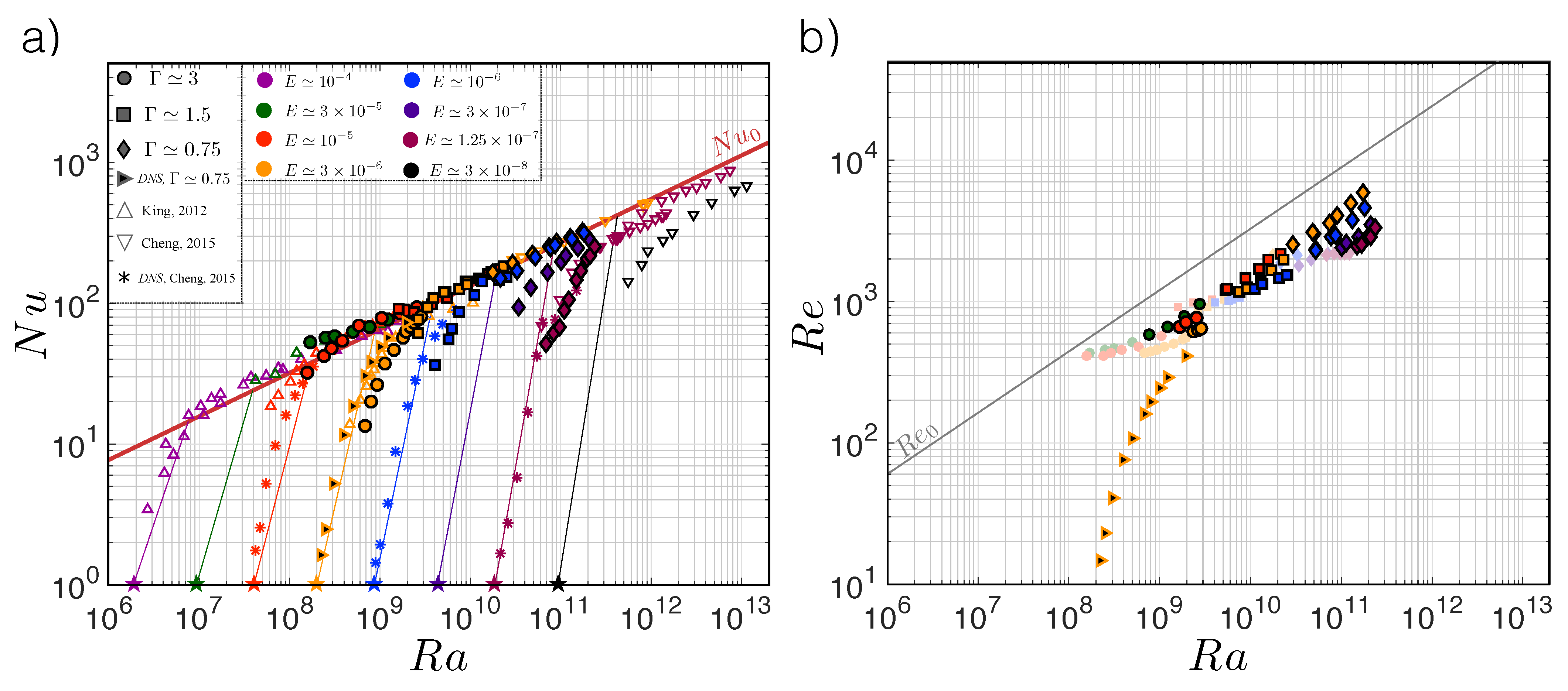
4.1. RBC Heat and Momentum Transfer Measurements

Figure 4a shows our RBC heat transfer results, along with the data from [64,65]. The Nusselt number, $Nu$, is displayed on the y-axis and the Rayleigh number, $Ra$, is shown on the x-axis. Pink and cyan markers represent our data, where symbol shapes represent the different tanks used: circles ($\Gamma \simeq 3$), squares ($\Gamma \simeq 1.5$), and diamonds ($\Gamma \simeq 0.75$). The $\Gamma \simeq 3$ data are distinguished in pink from the data collected in the $\Gamma \simeq 1.5$ and $\Gamma \simeq 0.75$ tanks (cyan) due to the different location of velocity measurements in the $\Gamma \simeq 3$ tank. The open gray triangles [64] and open upside-down gray triangles [65] are water data collected using UCLA’s smaller-diameter RoMag device. The fuchsia line in Figure 4a, $N{u}_0=0.108R{a}^{0.309}$, represents the best fit to our data. The scaling exponent, $\alpha =0.309\pm 0.003$, and pre-factor, $c=0.108\pm 0.009$, are in good agreement with those found in Cheng et al. [45]: $\alpha =0.308$ and $c=0.11$.

The RBC momentum transfer results of this study are shown in Figure 4b, with the Reynolds number, $Re$, displayed on the y-axis and the Rayleigh number, $Ra$, shown on the x-axis. The solid black line, $R{e}_0=(0.150\pm 0.052)R{a}^{(0.434\pm 0.012)}$, shows the best fit to the $\Gamma \simeq 1.5$ (squares) and $\Gamma \simeq 0.75$ (diamonds) data collected at $h_{\mathrm{ldv}}\simeq 0.57H$, $r_{\mathrm{ldv}}\simeq 0.84R$. This fit is in adequate agreement with the best fit of the experimental water data from Qiu and Tong [77]: $R{e}_0^{*}=0.102R{a}^{0.447}$.

The $\Gamma \simeq 3$ pink data collected at $h_{\mathrm{ldv}}\simeq 0.33H$, $r_{\mathrm{ldv}}\simeq 0.84R$ does not follow the same scaling behavior as in our other two tanks. This is likely due to the difference in the location of the point velocity measurements and the regime of convection probed. In all of the RBC experiments, a large-scale overturning circulation (LSC) pattern should exist in the fluid bulk. The velocity field of such an LSC structure is non-uniform (aka position dependent) within the fluid bulk (e.g., [71,77,158,159,160,161]). It is possible that the $\Gamma \simeq 3$ data at a non-dimensional height of $h_{\mathrm{ldv}}\simeq 0.33H$ samples a corner of an LSC structure, whereas the rest of our data at a height of $h_{\mathrm{ldv}}\simeq 0.57H$ (and larger $Ra$) measure velocities nearer to the center of the vertical upwellings and downwellings that comprise the LSC. Overall, our RBC heat and momentum transfer measurements agree well with the results of prior studies.

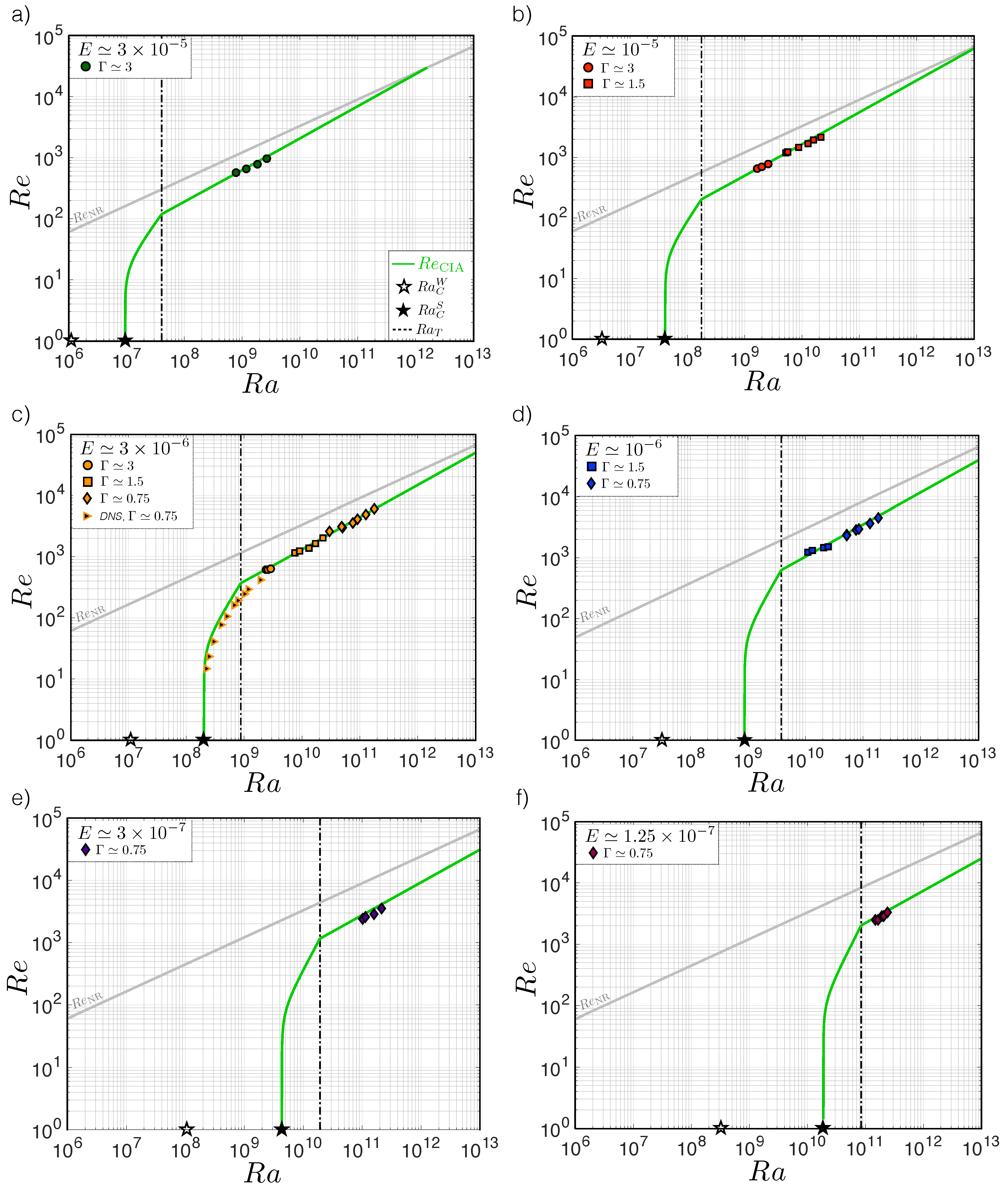
4.2. RRBC Heat and Momentum Transfer Measurements

Figure 5a shows $Nu$ versus $Ra$ for our RRBC heat transfer measurements. Symbol color represents the non-dimensional rotation period, E. The different symbol shapes represent the data collected in the three different experimental containers used in this study and are consistent with Figure 4. The $E\simeq 3\times {10}^{-6}$ DNS are displayed in Figure 5 as right pointing orange triangles with a black center. The open triangles represent data from [64], the open upside-down triangles represent data from [65], and the asterisks denote the direct numerical simulations from [65]. The onset values for steady bulk convection, given by (11), are shown as solid, colored stars on the x-axis. The colored, thin solid lines characterize the heat transfer regime occurring near the onset of convection given by (12) and (13). The numerical simulations reach closest to onset and provide the most data in this regime. The thick solid fuchsia line represents the best fit to the RBC data from Figure 4a.

Cheng et al. [65] note that it is possible that their two most extreme datasets at $E\simeq {10}^{-7}$ and $E\simeq 3\times {10}^{-8}$ might be influenced by strong centrifugal acceleration, which scaled as ${\Omega }^{2}R$. This may also be the case for our burgundy data at $E\simeq 1.25\times {10}^{-7}$ ($Fr\simeq 1\ge (\Gamma /2=0.375)$,81]). However, our $E\simeq 1.25\times {10}^{-7}$ data agree well with the $E\simeq {10}^{-7}$ numerics of [47] in which there is no centrifugal buoyancy. Thus, it is not obvious that the overall scaling behavior of this heat transfer data is altered by centrifugation (c.f. [9,45,162,163]). We conclude that our heat transfer data (both experimental and numerical) adequately agree with prior studies.

Figure 5b shows the $Re$ versus $Ra$ data for our RRBC experiments and DNS. The color and symbol shape are the same as those in Figure 5a, with one difference: faded symbols represent experimental data with measured velocities that are below the determined resolution limit of 2.5 mm/s for the LDV device used in this study (see Section 3.2). The solid, colored symbols thus represent the experimental velocity data above the 2.5 mm/s LDV device resolution limit that are used in the analysis of the RRBC momentum transfer data discussed below. The solid, faded black line is the best fit to the RBC momentum transfer data shown in Figure 4b, and serves as an upper bound for our rotating data. We note that the burgundy data ($E\simeq {10}^{-7}$, $Fr\simeq 1$) in Figure 5b do not show any observable influence of centrifugal buoyancy on vertical momentum transport.

Figure 6a displays the ratio of boundary layer thickness estimates, ${\delta }_E/{\delta }_T^{\mathrm{NR}}$, versus the $Ra$ for the laboratory data. The RBC thermal boundary layer thickness, ${\delta }_T^{\mathrm{NR}}$, is estimated using ${\delta }_T^{\mathrm{NR}}=H/\left(2Nu\right)$ given by (15) and the Ekman layer thickness, ${\delta }_E$, is estimated using ${\delta }_E=3E^{1/2}H$ given by (16) such that ${\delta }_E/{\delta }_T^{\mathrm{NR}}=6Nu{E}^{1/2}$. Previous studies have shown that whether RRBC heat transfer will behave as though the system is non-rotating versus being rotationally constrained depends on the overall dominance of an Ekman or a non-rotating thermal boundary layer in the system [21,46,47,64,89,164]. Thus, in Figure 6a we use hollow, colored symbols when ${\delta }_E/{\delta }_T^{\mathrm{NR}}\le 1$, and symbols become solid when ${\delta }_E/{\delta }_T^{\mathrm{NR}}>1$.

Figure 6b displays the laboratory $Nu$ data normalized by our empirical non-rotating style scaling, $N{u}_0=0.108R{a}^{0.309}$, plotted versus $Ra$. The same symbol significance used in Figure 6a is used here, that is, symbols are hollow if ${\delta }_E/{\delta }_T^{\mathrm{NR}}\le 1$ and solid if ${\delta }_E/{\delta }_T^{\mathrm{NR}}>1$. We see that the symbols are hollow when $Nu/N{u}_0\lesssim 1$, whereas the symbols become solid roughly when $Nu/N{u}_0$ becomes unity. Thus, when ${\delta }_E/{\delta }_T^{\mathrm{NR}}\le 1$, the Ekman layer remains thin, resulting in rotationally constrained heat transfer behavior. Contrastingly, when $Nu/N{u}_0$ roughly becomes unity, the thermal boundary layer becomes thinner than the Ekman layer and non-rotating-style heat transfer behavior is recovered. We conclude that the behavioral transitions in our RRBC heat transfer data correlate to the boundary layer physics of the system, consistent with prior studies (e.g., [22,47,59,128]).

Figure 7 shows the measured $Re$ values from Figure 5b with the scaling predictions from Figure 2d separately for each fixed E dataset. Note that only the laboratory data that are above the LDV device resolution limit are included in each panel in Figure 7. Experimental data below the LDV device resolution limit (faded symbols in Figure 5b) are not included in any of the ensuing momentum transfer analysis. The inclusion of the orange $E\simeq 3\times {10}^{-6}$ DNS in panel c in Figure 7 allows us to examine the $Re$ behavior closer to the onset of convection than is possible with the laboratory experiments.

The empirical best fits of $N{u}_0$ and $N{u}_{\Omega }$ from Figure 5a are used in the computation of the green $Re$ CIA theoretical curves shown in each panel in Figure 7 and given by (24). Specifically, below $Ra\le R{a}_T$, $N{u}_{\Omega }$ is used in the calculation of these green curves, and above $Ra>R{a}_T$, $N{u}_0$ is used. A pre-factor of unity is assumed in the calculation of these curves. All of our measured laboratory $Re$ values align well with the green CIA $Re$ scaling predictions for each fixed E dataset in Figure 7. The DNS in panel c have decent agreement with the theoretical CIA prediction. We note that full volume average calculations of the DNS $Re$ values more directly overlay onto the green CIA theory curve in panel c.

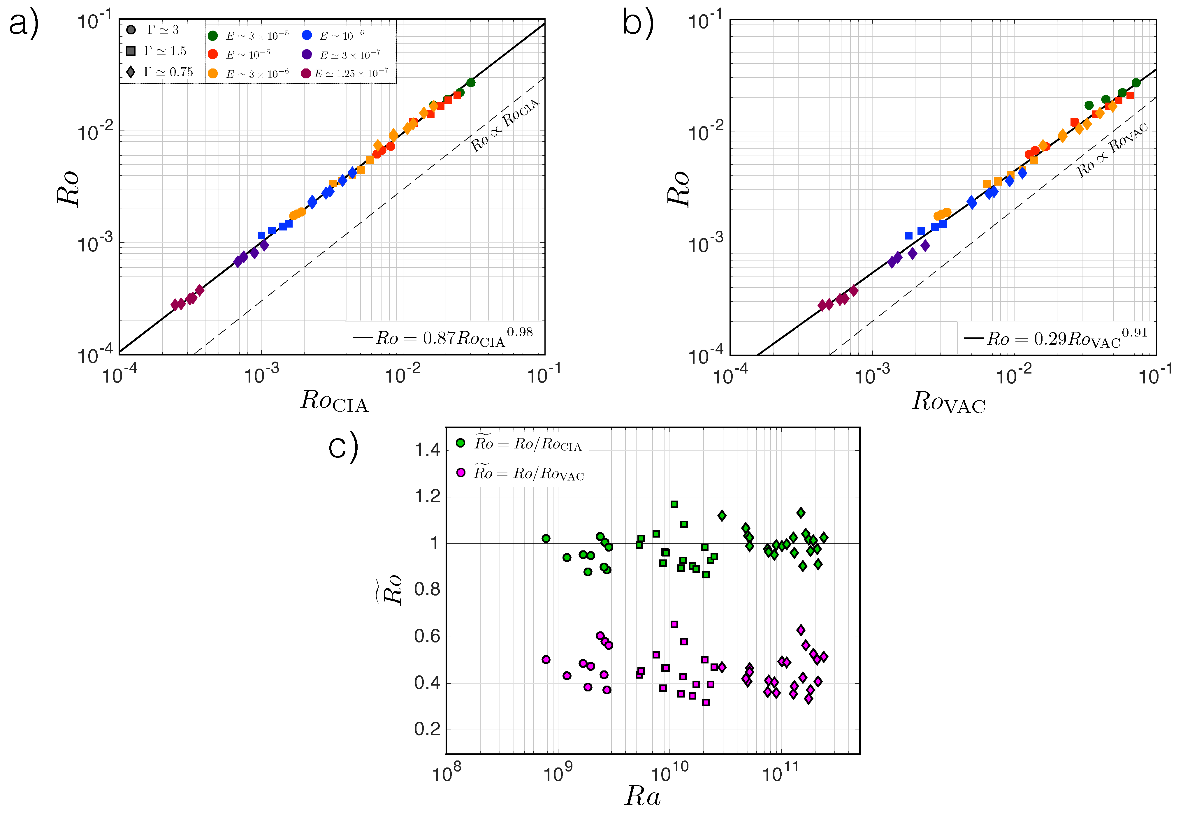
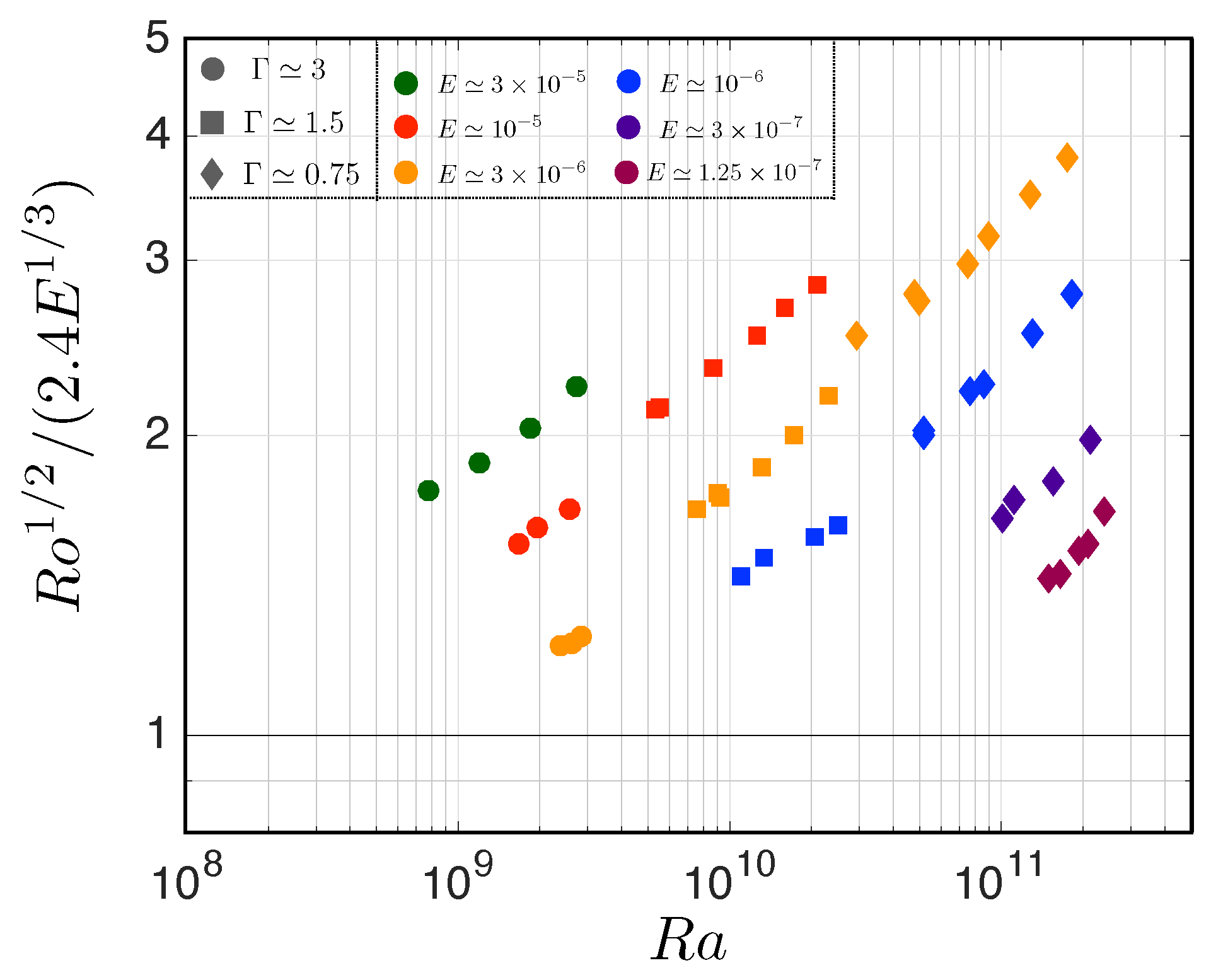
4.2.1. Co-Scaling of the VAC and CIA Predictions

Figure 8a shows measured $Ro$ versus the $R{o}_{\mathrm{CIA}}$. A best fitfit line on this graph yields $Ro=(0.87\pm 0.03){R{o}_{\mathrm{CIA}}}^{(0.98\pm 0.01)}$, indicating excellent agreement between experimental velocity measurements and associated predictions using the triple-balance assumption of the CIA scaling given by (24). Thus, our velocity measurements indicate that the Coriolis force, inertial advection, and buoyancy control the bulk momentum transport. Figure 8b displays measured $Ro$ versus the $R{o}_{\mathrm{VAC}}$. Decent agreement also exists between LDV measurements and associated VAC predictions. Specifically, a best fitfit line on this graph yields $Ro=(0.29\pm 0.02){R{o}_{\mathrm{VAC}}}^{(0.91\pm 0.01)}$. The VAC scaling prediction given by (21) assumes that viscous diffusion, instead of inertial advection, acts in balance with the Coriolis force and buoyancy to control the momentum transport.

Figure 8a,b indicate that both the VAC and CIA scalings of $Re$ given by (21) and (24) adequately predict momentum transport behavior. To further highlight this, Figure 8c shows normalized Rossby numbers, $\widetilde{Ro}$, versus $Ra$. $\widetilde{Ro}$ is defined as laboratory LDV values normalized by either CIA estimates, $\widetilde{Ro}=Ro/R{o}_{\mathrm{CIA}}$ (green), or by VAC estimates, $\widetilde{Ro}=Ro/R{o}_{\mathrm{VAC}}$ (magenta). The green $Ro/R{o}_{\mathrm{CIA}}$ points are well-centered around 1, indicating that the CIA scaling estimates our measured convective velocities well, as expected from the excellent best fit shown in Figure 8a. The magenta $Ro/R{o}_{\mathrm{VAC}}$ points show that the VAC scaling overestimates measured values of $Ro$ by roughly a factor of 2. The magenta VAC normalized points contain an overall flat slope, similar to that of the green CIA normalized points, indicating that the VAC scaling also captures the velocity behavior of the system, even if offset by a small, constant factor.

We conclude from Figure 8 that the CIA scaling predictions fit our data extremely well, in good agreement with the findings from planetary dynamo models (cf. [4,33,34,165,166]). No pre-factors are used in the calculations of the CIA and VAC scaling predictions given by (24) and (21), respectively. Importantly, the VAC scaling also fits our velocity data reasonably well over the full range of $Ra$ investigated. Thus, the CIA and VAC scalings appeared to co-scale, with both adequately predicting the measured data.

The VAC and CIA momentum transfer scalings only differed in the assumed cross-axial length scale of the flow. This length scale is not directly measured in this study. We estimate the local onset and turbulent scales using (20) and (22), respectively. Figure 9 shows the ratio of these two length scales, $R{o}^{1/2}/\left(2.4E^{1/3}\right)$, plotted versus $Ra$ for our RRBC experimental data. The ratio of the length scales in Figure 9 only differs by a factor of 4. Thus, the onset scale, ${\ell }_{\mathrm{crit}}$, associated with the VAC scaling and the turbulent scale, ${\ell }_{\mathrm{turb}}$, associated with the CIA scaling are not formally scaled separately in the range of the parameter space explored experimentally (cf. [28,167,168,169]). This is also the case for the DNS in this study.

We conclude from Figure 9 that the VAC and CIA scalings both explained our velocity data because their underlying length scales are closely comparable in value. Thus, Figure 8 and Figure 9 lead us to postulate that the two scalings of ℓ discussed, the onset scale, ${\ell }_{\mathrm{crit}}$, and the inertial scale, ${\ell }_{\mathrm{turb}}$, must be comparable in this study. We now demonstrate that when local bulk Reynolds numbers, $R{e}_{\ell }$, are moderate (e.g., mathematically order unity) and local bulk Rossby numbers remain small (i.e., $R{o}_{\ell }\lesssim \mathcal{O}\left(1\right)$), the two length scales that define the VAC and CIA scalings, respectively, ${\ell }_{\mathrm{crit}}$ and ${\ell }_{\mathrm{turb}}$, will co-scale. In Section 4.2.2, we demonstrate that these two conditions are satisfied, i.e., $R{e}_{\ell }\sim \mathcal{O}({10}^1-{10}^2)$ and $R{o}_{\ell }\lesssim \mathcal{O}\left(1\right)$, for our RRBC laboratory data. Thus, the following analysis holds true for our experiments.

Using ${\ell }_{\mathrm{crit}}\sim E^{1/3}H$, the local Reynolds number can be defined as:

$$R{e}_{\ell }=\frac{u{\ell }_{\mathrm{crit}}}{\nu }\sim Re{E}^{1/3}.$$

(28)

Assuming that the local Reynolds number is mathematically of order unity, i.e.:

$$R{e}_{\ell }\sim Re{E}^{1/3}\sim \mathcal{O}\left(1\right),$$

(29)

and since $Ro=ReE$, then,

$$Ro\sim (R{e}_{\ell }{E}^{-1/3})E\sim E^{2/3}.$$

(30)

Using (30), we see that the inertial scale, ${\ell }_{\mathrm{turb}}\sim R{o}^{1/2}H$, scales equivalently to the onset scale:

$$\ell \sim R{o}^{1/2}H\sim {\left(E^{2/3}\right)}^{1/2}H\sim E^{1/3}H.$$

(31)

Thus, we crucially note that when $R{e}_{\ell }\sim \mathcal{O}\left(1\right)$ in RRBC systems, the onset and turbulent cross-axial scales are comparable, i.e.: (cf. [28,31,32,34])

$$\ell \sim E^{1/3}H\sim R{o}^{1/2}H.$$

(32)

The VAC scaling of (21) and the CIA scaling of (24) are thus comparable:

$$R{e}_{\mathrm{VAC}}\sim R{e}_{\mathrm{CIA}}.$$

(33)

From the above analysis and Figure 8 and Figure 9, we conclude that the bulk dynamics are robustly governed by a Coriolis–Inertia–Archimedian (buoyancy) balance in the range of $Ra$ explored in this study (cf. [4,34,53,59,170]), while ${\ell }_{\mathrm{turb}}$ never departs significantly from ${\ell }_{\mathrm{crit}}$. We purport that viscous forces act secondarily on bulk dynamics under the CIA balance (cf. [89]), and either length scale estimate can be used to accurately predict the cross-axial scale of flows.

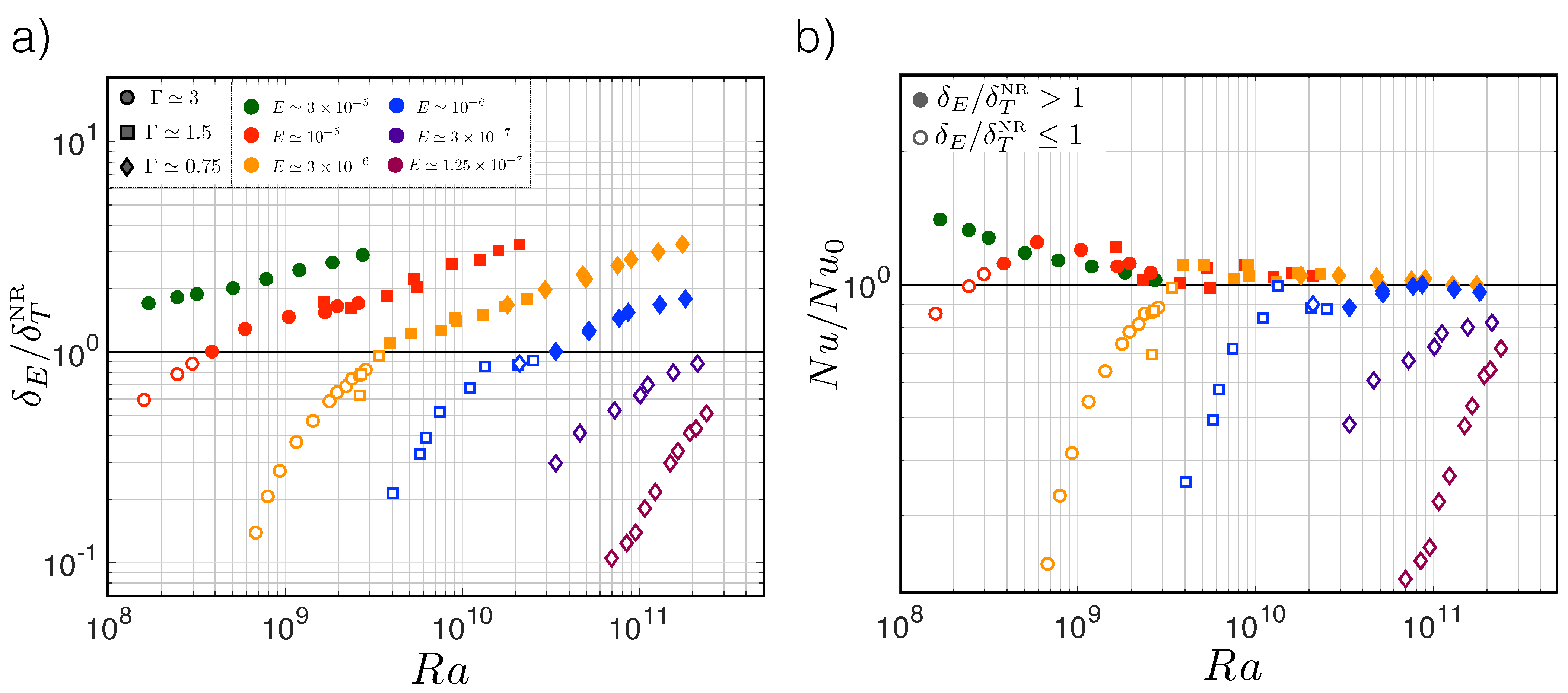
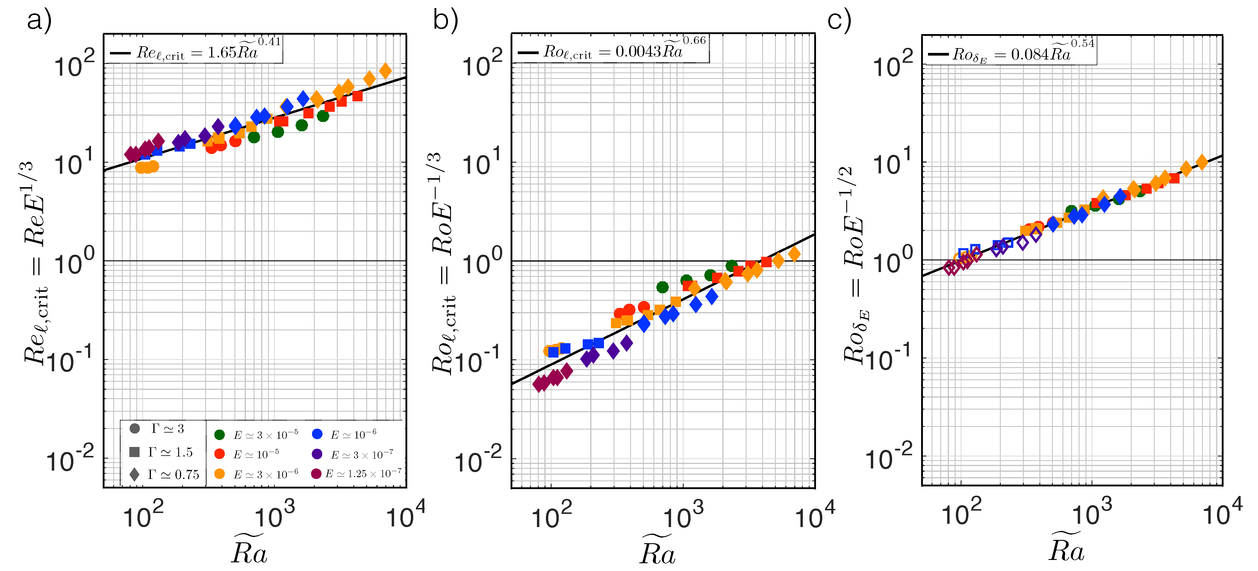
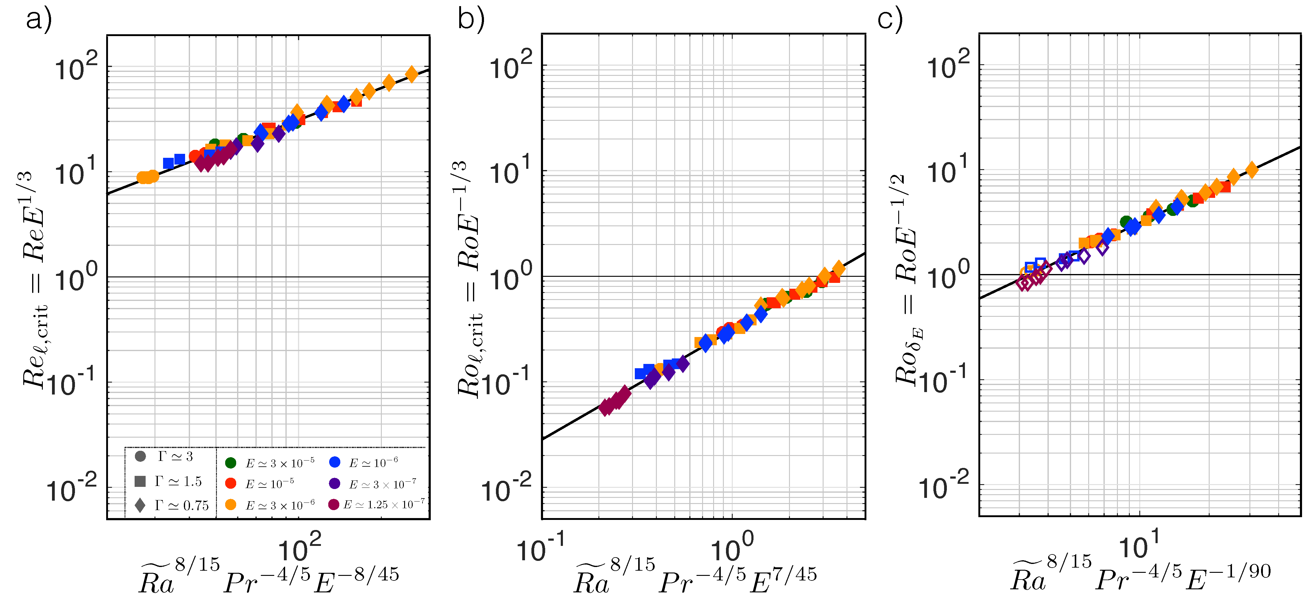
4.2.2. Local Flow Estimates and Comparison to Asymptotic Theory

Figure 8 and Figure 9 motivate further exploration of local estimates within the bulk and boundary layers of our experiments. Using the onset scale given by (20) for ℓ, a local Reynolds number for the fluid bulk can be defined as:

$$R{e}_{\ell ,\mathrm{crit}}=\frac{u{\ell }_{\mathrm{crit}}}{\nu }=Re{E}^{1/3},$$

(34)

where $Re$ is the global Reynolds number computed by (27) for our experiments. The definition of $R{e}_{\ell ,\mathrm{crit}}$ in (34) does not use any empirical pre-factors for simplicity. Figure 10a displays $R{e}_{\ell ,\mathrm{crit}}$ versus $\widetilde{Ra}=Ra{E}^{4/3}\simeq Ra/R{a}_C^S$, a measure of the convective supercriticality of experiments. Color and symbol shape are consistent with that of Figure 9, and the best fit black line is given as $R{e}_{\ell ,\mathrm{crit}}=(1.65\pm 0.25){\widetilde{Ra}}^{(0.41\pm 0.02)}$. Bulk local $Re$ estimates are $\mathcal{O}({10}^1-{10}^2)$. Note that the turbulent length scale given by (22) can instead be used for ℓ in (34) and approximately identical results are obtained.

We define a local bulk Rossby number as:

$$R{o}_{\ell ,\mathrm{crit}}=\frac{u}{2\Omega {\ell }_{\mathrm{crit}}}=Ro{E}^{-1/3}.$$

(35)

Figure 10b displays $R{o}_{\ell ,\mathrm{crit}}$ versus $\widetilde{Ra}$, where the best fit black line is given as $R{o}_{\ell ,\mathrm{crit}}=(0.0043\pm 0.0009){\widetilde{Ra}}^{(0.66\pm 0.03)}$. Bulk local $Ro$ estimates remain small, i.e., $R{o}_{\ell ,\mathrm{crit}}\lesssim 1$. Quasi-geostrophic turbulence exists in the fluid bulk when $R{e}_{\ell }\gtrsim \mathcal{O}\left(10\right)$ and $R{o}_{\ell }\lesssim 1$ (e.g., [5,52,167,171,172,173,174]). Thus, collectively, Figure 10a,b indicate, via local arguments of the fluid bulk, that the experiments plotted possess quasi-geostrophically turbulent bulk dynamics, consistent with the global analysis highlighted in Figure 8.

Local boundary layer dynamics are explored in Figure 10c, which displays $R{o}_{{\delta }_E}$ versus $\widetilde{Ra}$. $R{o}_{{\delta }_E}$ is a local Rossby number in the fluid boundary layers that we define as:

$$R{o}_{{\delta }_E}=\frac{u}{2\Omega {\delta }_E}=Ro{E}^{-1/2},$$

(36)

where ${\delta }_E$ is the Ekman boundary layer thickness given by (16). No pre-factor is used in our definition of (36) above. The hollow symbols in Figure 10c indicate cases in which the rotational effects dominate the boundary layers according to the criteria in Figure 6, i.e., ${\delta }_E/{\delta }_T^{\mathrm{NR}}\le 1$. Comparing the number of hollow data points in Figure 6 versus those in Figure 10c, we see that there are fewer hollow points in Figure 10c (but the same number of solid points in the two figures). The reason for this is that the velocity data points that are below the LDV device resolution limit are not displayed in Figure 10c. Many of the velocity data points below this resolution limit exist in the heat transfer regime that is controlled by rotation. Figure 10c shows that estimated local $Ro$ values within the Ekman boundary layers are greater than unity for the majority of the data shown, confirming that boundary layer dynamics are not strongly controlled by rotation. We note that plotting $R{o}_{{\delta }_E}$ versus $\widetilde{Ra}$, as in Figure 10c, results in well-collapsed data, with a best fit black line given as $R{o}_{{\delta }_E}=(0.084\pm 0.005){\widetilde{Ra}}^{(0.54\pm 0.01)}$.

According to asymptotic theory, diffusion-free heat transfer should behave as: [5,18,50,58,98]

$$Nu\sim R{a}^{3/2}{E}^{2}P{r}^{-1/2}.$$

(37)

This balance is not achieved in our experiments and DNS because the boundary layer physics controls heat transfer behavior in the parameter space explored. Following the flux-based scaling arguments of Aurnou et al. [53], the diffusion-free CIA estimate of the global Reynolds number can be estimated using (37) as:

$$R{e}_{\mathrm{CIA}}\sim {\left(\frac{RaNu}{P{r}^2}\right)}^{\frac{2}{5}}{E}^{\frac{1}{5}}\sim {\left(\frac{Ra}{P{r}^2}\frac{R{a}^{3/2}{E}^2}{P{r}^{1/2}}\right)}^{\frac{2}{5}}{E}^{\frac{1}{5}}\sim \frac{RaE}{Pr}.$$

(38)

Taking $R{e}_{\mathrm{CIA}}$ as an estimate of the global Reynolds number, the scaling predictions for the local estimate parameters displayed in Figure 10 are:

$$\begin{array}{c}\hfill R{e}_{\ell ,\mathrm{crit}}=R{e}_{\mathrm{CIA}}{E}^{1/3}\simeq \frac{RaE}{Pr}{E}^{1/3}=\frac{\widetilde{Ra}}{Pr},\end{array}$$

(39a)

$$\begin{array}{c}\hfill R{o}_{\ell ,\mathrm{crit}}=\left(R{e}_{\mathrm{CIA}}E\right)E^{-1/3}\simeq \frac{RaE}{Pr}{E}^{2/3}=\frac{\widetilde{Ra}{E}^{1/3}}{Pr},\end{array}$$

(39b)

$$\begin{array}{c}\hfill R{o}_{{\delta }_E}=\left(R{e}_{\mathrm{CIA}}E\right)E^{-1/2}\simeq \frac{RaE}{Pr}{E}^{1/2}=\frac{\widetilde{Ra}{E}^{1/6}}{Pr}.\end{array}$$

(39c)

Thus, in the asymptotic diffusion-free limit, local estimates all scale with ${\widetilde{Ra}}^1$. This scaling is not seen in panels a–c of Figure 10. However, we do not expect these asymptotic scalings to hold in our data since the diffusion-free heat transfer regime given by (37) is not attained.

If we re-do the above analysis using the experimental heat transfer relation found herein, $Nu\sim R{a}^{1/3}$, rather than (37), the CIA scaling of $Re$ now becomes:

$$R{e}_{\mathrm{CIA}}\sim {\left(\frac{RaNu}{P{r}^2}\right)}^{\frac{2}{5}}{E}^{\frac{1}{5}}\sim {\left(\frac{RaR{a}^{1/3}}{P{r}^2}\right)}^{\frac{2}{5}}{E}^{\frac{1}{5}}\sim \frac{{\widetilde{Ra}}^{8/15}}{P{r}^{4/5}}{E}^{-23/45}.$$

(40)

Thus, we predict that $R{e}_{\ell ,\mathrm{crit}}$, $R{o}_{\ell ,\mathrm{crit}}$, and $R{o}_{{\delta }_E}$ will experimentally scale with $\widetilde{Ra}$ as:

$$\begin{array}{c}\hfill R{e}_{\ell ,\mathrm{crit}}=R{e}_{\mathrm{CIA}}{E}^{1/3}\simeq {\widetilde{Ra}}^{8/15}{Pr}^{-4/5}{E}^{-8/45},\end{array}$$

(41a)

$$\begin{array}{c}\hfill R{o}_{\ell ,\mathrm{crit}}=\left(R{e}_{\mathrm{CIA}}E\right)E^{-1/3}\simeq {\widetilde{Ra}}^{8/15}{Pr}^{-4/5}{E}^{7/45},\end{array}$$

(41b)

$$\begin{array}{c}\hfill R{o}_{{\delta }_E}=\left(R{e}_{\mathrm{CIA}}E\right)E^{-1/2}\simeq {\widetilde{Ra}}^{8/15}{Pr}^{-4/5}{E}^{-1/90}.\end{array}$$

(41c)

Figure 11a shows the local Reynolds number, $R{e}_{\ell ,\mathrm{crit}}$, plotted against Equation (41a). Similarly, Figure 11b displays the local Rossby number, $R{o}_{\ell ,\mathrm{crit}}$, plotted versus Equation (41b), and Figure 11c shows the local boundary layer Rossby number, $R{o}_{{\delta }_E}$, versus Equation (41c). All data in each panel collapse in y, indicating that each prediction of its respective local estimate is accurate. Further, the best fit black lines all yield a fit of $y\simeq 0.3x^{1.0}$. Thus, boundary layer controlled heat transfer and inviscid, quasi-geostrophic bulk dynamics provide accurate predictions of local parameters in both the bulk and boundary layers of experiments.

5. Discussion

The results of a laboratory-numerical survey of rotating Rayleigh–Bénard convection in which the heat and momentum transfer are simultaneously measured are presented. Thermal measurements are collected to characterize convective heat transfer in conjunction with measurements of fluid bulk convective-point velocities via laser Doppler velocimetry. For non-rotating experiments, data agree well with those of past studies, thus validating the convective measurements in this work. Specifically, non-rotating heat transfer data scale as $Nu\sim R{a}^{1/3}$ while the momentum transfer measurements exhibit a $Re\sim R{a}^{1/2}$ scaling.

Rotating convection DNS and laboratory heat transfer data show that transitions in heat transfer behavior are determined by boundary layer dynamics. Bulk dynamics are robustly governed by the inviscid CIA balance. Simultaneous measurements of heat and momentum transfer show that the CIA $Re$ scaling holds from near convective onset to nearly ∼800 times critical (at low E, i.e., $E\simeq 3\times {10}^{-6}$). Importantly, this velocity behavior is not correlated with boundary layer dynamics, unlike heat transfer behavior. The onset and turbulent length scale estimates co-scale such that the VAC and CIA scalings of $Re$ co-scale when the local Reynolds number in the fluid bulk is of order unity. We argue that this explains the results shown in Figure 8 and Figure 9. An open question remains as to if, and under what conditions, the theoretical viscous and inertial length scales of RRBC underlying the VAC and CIA velocity scalings become clearly scale separable (e.g., [24,175,176,177]).

An analysis of the local flow estimates of our experiments also shows that bulk flow dynamics display properties of quasi-geostrophic turbulence. Local bulk Reynolds numbers are large while local bulk Rossby numbers remain small. Estimates of the local Reynolds numbers in the boundary layers are of order unity and demonstrate that heat transfer behavior is intimately tied to boundary layer dynamics. Thus, an analysis of local flow dynamics conveys the same findings as a global analysis. Further, the relationship between local estimates and convective supercriticality is properly accounted for by considering both boundary layer dominated heat transfer and inviscid bulk dynamics.

Quasi-geostrophic turbulence, relevant to dynamo flows, develops in the fluid bulk of experiments, even relatively near to onset. This finding suggests that we can access diffusion-free bulk dynamics in models that are far from planetary core conditions. Cheng and Aurnou [139] asserted that dynamo models cannot be extrapolated to core conditions because the heat transfer in these models is not diffusion-free. Meanwhile, many dynamo models exhibit diffusion-free CIA-balanced flow dynamics (e.g., [4,34,165,166]). Our findings elucidate that although the heat transfer in these models remains controlled by boundary layer dynamics, diffusion-free bulk flow dynamics are indeed captured.

Over the nearly 100 years in which laboratory convection experiments have been conducted, a long-standing assumption has been that heat transfer behavior is indicative of the full system dynamics (cf. [38,41,88,96]). This study clarifies that laboratory studies and comparable numerical work contain boundary layer controlled heat transfer that prevents bulk dynamics from becoming fully diffusion-free. The CIA $Re$ scaling is dependent on heat transfer via $Nu$. Thus, bulk flows in present-day laboratory-numerical models contain inviscid, CIA-balanced flow dynamics that are limited by boundary layer controlled heat transfer [36].

Another interesting outstanding question remains as to the conditions under which present-day DNS and laboratory models might be able to achieve diffusion-free heat transfer. A recent laboratory study by Bouillaut et al. [163] claims to find the diffusion-free heat transfer scaling, $Nu\sim R{a}^{3/2}{E}^{2}P{r}^{-1/2}$, using radiatively driven convection. Overall, the work herein illuminates that boundary layer processes throttle the dynamics in current RRBC laboratory experiments. This boundary layer throttling prohibits the observation of the asymptotic RRBC flow state described by (38), which likely dominates in planetary cores [53].

References

1. Elsassar, W. On the Origin of the Earth’s Magnetic Field. Phys. Rev. 1939, 55, 489–498. [Google Scholar] [CrossRef]
2. Roberts, P.H.; King, E.M. On the genesis of the Earth’s magnetism. Rep. Prog. Phys. 2013, 76, 096801. [Google Scholar] [CrossRef] [PubMed] [Green Version]
3. Cheng, J.S.; Aurnou, J.M.; Julien, K.; Kunnen, R. A heuristic framework for next-generation models of geostrophic convective turbulence. Geophys. Astrophys. Fluid Dyn. 2018, 112, 277–300. [Google Scholar] [CrossRef] [Green Version]
4. Schwaiger, T.; Gastine, T.; Aubert, J. Relating force balances and flow length scales in geodynamo simulations. Geophys. J. Int. 2021, 224, 1890–1904. [Google Scholar] [CrossRef]
5. Maffei, S.; Krouss, M.; Julien, K.; Calkins, M. On the inverse cascade and flow speed scaling behaviour in rapidly rotating Rayleigh-Bénard convection. J. Fluid Mech. 2021, 913, A18. [Google Scholar] [CrossRef]
6. Horn, S.; Schmid, P.J. Prograde, Retrograde, and Oscillatory modes in rotating Rayleigh-Bénard Convection. J. Fluid Mech. 2017, 831, 182–211. [Google Scholar] [CrossRef] [Green Version]
7. Aurnou, J.; Bertin, V.; Grannan, A.; Horn, S.; Vogt, T. Rotating thermal convection in liquid gallium: Multi-modal flow, absent steady columns. J. Fluid Mech. 2018, 846, 846–876. [Google Scholar] [CrossRef] [Green Version]
8. Aujogue, K.; Pothérat, A.; Sreenivasan, B.; Debray, F. Experimental study of the convection in arotating tangent cylinder. J. Fluid Mech. 2018, 843, 355–381. [Google Scholar] [CrossRef] [Green Version]
9. de Wit, X.; Guzman, A.A.; Madonia, M.; Cheng, J.S.; Clercx, H.; Kunnen, R. Turbulent rotating convection confined in a slender cylinder: The sidewall circulation. Phys. Fluid Dyn. 2020, 5, 023502. [Google Scholar] [CrossRef] [Green Version]
10. Lu, H.; Ding, G.; Shi, J.; Xia, K.; Zhong, J. Heat-transport scaling and transition in geostrophic rotating convection with varying aspect ratio. Phys. Rev. Fluids 2021, 6, L071501. [Google Scholar] [CrossRef]
11. Ecke, R.E.; Zhang, X.; Shishkina, O. Connecting wall modes and boundary zonal flows in rotating Rayleigh-Bénard convection. Phys. Rev. Fluids 2022, 7, L011501. [Google Scholar] [CrossRef]
12. Wedi, M.; Moturi, V.; Funfschilling, D.; Weiss, S. Experimental evidence for the boundary zonal flow in rotating Rayleigh-Bénard convection. J. Fluid Mech. 2022, 939, A14. [Google Scholar] [CrossRef]
13. Gastine, T.; Aurnou, J.M. Latitudinal regionalization of rotating spherical shell convection. J. Fluid Mech. 2022, 954, R1. [Google Scholar] [CrossRef]
14. Wang, G.; Santelli, L.; Lohse, D.; Verzicco, R.; Stevens, R. Diffusion-free scaling in rotating spherical Rayleigh Bénard Convection. Geophys. Res. Lett. 2021, 48, e2021GL095017. [Google Scholar] [CrossRef]
15. Sheyko, A.; Finlay, C.; Favre, J.; Jackson, A. Scale separated low viscosity dynamos and dissipation within the Earth’s core. Sci. Rep. 2018, 8, 12566. [Google Scholar] [CrossRef] [PubMed]
16. Ecke, R.E.; Shishkina, O. Turbulent Rotating Rayleigh-Bénard Convection. Ann. Rev. Fluid Mech. 2023, 55, 603–638. [Google Scholar] [CrossRef]
17. Kunnen, R. The geostrophic regime of rapidly rotating turbulent convection. J. Turbul. 2021, 22, 267–296. [Google Scholar] [CrossRef]
18. Sprague, M.; Julien, K.; Knobloch, E.; Werne, J. Numerical simulation of an asymptotically reduced system for rotationally constrained convection. J. Fluid Mech. 2006, 551, 141–174. [Google Scholar] [CrossRef]
19. Kunnen, R.; Geurts, B.; Clercx, H. Experimental and numerical investigation of turbulent convection in a rotating cylinder. J. Fluid Mech. 2010, 642, 445–476. [Google Scholar] [CrossRef]
20. King, E.; Aurnou, J.M. Thermal evidence for Taylor columns in turbulent rotating Rayleigh-Bénard convection. Phys. Rev. E 2012, 85, 016313. [Google Scholar] [CrossRef] [Green Version]
21. Julien, K.; Rubio, A.M.; Grooms, I.; Knobloch, E. Statistical and physical balances in low-Rossby-number Rayleigh-Bénard convection. Geophys. Astrophys. Fluid Dyn. 2012, 106, 392–428. [Google Scholar] [CrossRef]
22. Gastine, T.; Wicht, J.; Aubert, J. Scaling regimes in spherical shell rotating convection. J. Fluid Mech. 2016, 808, 690–732. [Google Scholar] [CrossRef] [Green Version]
23. Chong, K.; Yang, Y.; Haung, S.; Zhong, J.; Stevens, R.; Verzicco, R.; Lohse, D.; Xia, K. Confined Rayleigh–B’enard, rotating Rayleigh–B’enard, and double diffusive convection: A unifying view on turbulent transport enhancement through coherent structure manipulation. Phys. Rev. Lett. 2017, 119, 064501. [Google Scholar] [CrossRef] [PubMed] [Green Version]
24. Rajaei, H.; Alards, K.; Kunnen, R.; Clercx, H. Velocity and acceleration statistics in rapidly rotating Rayleigh–Bénard convection. J. Fluid Mech. 2018, 857, 374–397. [Google Scholar] [CrossRef]
25. Vogt, T.; Horn, S.; Aurnou, J. Oscillatory thermal-inertial flows in liquid metal rotating convection. J. Fluid Mech. 2021, 911, A5. [Google Scholar] [CrossRef]
26. Long, R.S. Regimes and Scaling Laws for Convection with and without Rotation. Ph.D. Thesis, The University of Leeds, Leeds, UK, 2021. [Google Scholar]
27. Soderlund, K.; King, E.; Aurnou, J.M. The influence of magnetic fields in planetary dynamo models. Earth Planet. Sci. Lett. 2012, 333, 9–20. [Google Scholar] [CrossRef]
28. Calkins, M.; Julien, K.; Tobias, S.; Aurnou, J. A multi-scale dynamo model driven by quasigeostrophic convection. J. Fluid Mech. 2015, 780, 143–166. [Google Scholar] [CrossRef] [Green Version]
29. Yadav, R.; Gastine, T.; Christensen, U.R.; Wolk, S.; Poppenhaeger, K. Approaching a realistic force balance in geodynamo simulations. Proc. Natl. Acad. Sci. USA 2016, 113, 12065–12070. [Google Scholar] [CrossRef] [Green Version]
30. Aurnou, J.; King, E. The cross-over to magnetostrophic convection in planetary dynamo systems. Proc. R. Soc. A 2017, 473, 20160731. [Google Scholar] [CrossRef] [Green Version]
31. Calkins, M. Quasi-geostrophic dynamo theory. Phys. Earth Planet. Inter. 2018, 276, 182–189. [Google Scholar] [CrossRef]
32. Aubert, J. Approaching Earth’s core conditions in high-resolution geodynamo simulations. Geophys. J. Int. 2019, 219, 137–151. [Google Scholar] [CrossRef]
33. Schwaiger, T.; Gastine, T.; Aubert, J. Force balance in numerical geodynamo simulations: A systematic study. Geophys. J. Int. 2019, 219, 101–114. [Google Scholar] [CrossRef]
34. Calkins, M.; Orvedahl, R.J.; Featherstone, N.A. Large-scale balances and asymptotic behaviour in spherical dynamos. Geophys. J. Int. 2021, 227, 1228–1245. [Google Scholar] [CrossRef]
35. Yan, M.; Tobias, S.; Calkins, M. Scaling behaviour of small-scale dynamos driven by Rayleigh-Bénard convection. J. Fluid Mech. 2021, 915, A15. [Google Scholar] [CrossRef]
36. Orvedahl, R.; Featherstone, N.A.; Calkins, M. Large-scale magnetic field saturation and the Elsasser number in rotating spherical dynamo models. Mon. Not. R. Astron. Soc. Lett. 2021, 507, 67–71. [Google Scholar] [CrossRef]
37. Kolhey, P.; Stellmach, S.; Heyner, D. Influence of boundary conditions on rapidly rotating convection and its dynamo action in a plane fluid layer. Phys. Rev. Fluids 2022, 7, 043502. [Google Scholar] [CrossRef]
38. Rossby, H.T. A study of Bénard convection with and without rotation. J. Fluid Mech. 1969, 36, 309–335. [Google Scholar] [CrossRef]
39. Kerr, R.M.; Herring, J.R. Prandtl number dependence of Nusselt number in direct numerical simulations. J. Fluid Mech. 2000, 419, 325–344. [Google Scholar] [CrossRef]
40. Funfschilling, D.; Brown, E.; Nikolaenko, A.; Ahlers, G. Heat transport by turbulent Rayleigh-Bénard convection in cylindrical samples. J. Fluid Mech. 2005, 536, 145–154. [Google Scholar] [CrossRef] [Green Version]
41. Weiss, S.; Stevens, R.; Zhong, J.; Clercx, H.; Lohse, D.; Ahlers, G. Finite-Size Effects Lead to Supercritical Bifurcations in Turbulent Rotating Rayleigh-Bénard Convection. Phys. Rev. Lett. 2010, 105, 224501. [Google Scholar] [CrossRef] [PubMed]
42. Choblet, G. On the scaling of heat transfer for mixed heating convection in a spherical shell. Phys. Earth Planet. Inter. 2012, 206, 31–42. [Google Scholar] [CrossRef]
43. Horn, S.; Shishkina, O. Rotating non-Oberbeck-Boussinesq Rayleigh-Bénard convection in water. Phys. Fluids 2014, 26, 055111. [Google Scholar] [CrossRef] [Green Version]
44. Ecke, R.E. Scaling of heat transport near onset in rapidly rotating convection. Phys. Lett. A 2015, 379, 2221–2223. [Google Scholar] [CrossRef] [Green Version]
45. Cheng, J.S.; Madonia, M.; Guzman, A.A.; Kunnen, R. Laboratory exploration of heat transfer regimes in rapidly rotating turbulent convection. Phys. Rev. Fluids 2020, 5, 113501. [Google Scholar] [CrossRef]
46. King, E.; Stellmach, S.; Noir, J.; Hansen, U.; Aurnou, J.M. Boundary layer control of rotating convection systems. Nature 2009, 457, 301–304. [Google Scholar] [CrossRef]
47. Stellmach, S.; Lischper, M.; Julien, K.; Vasil, G.; Cheng, J.S.; Ribeiro, A.; King, E.M.; Aurnou, J.M. Approaching the Asymptotic Regime of Rapidly Rotating Convection: Boundary Layers versus Interior Dynamics. Phys. Rev. Lett. 2014, 113, 254501. [Google Scholar] [CrossRef] [Green Version]
48. Stevenson, D. Turbulent thermal convection in the presence of rotation and a magnetic field: A hueristic theory. Geophys. Astrophys. Fluid Dyn. 1979, 12, 139–169. [Google Scholar] [CrossRef]
49. Julien, K.; Knobloch, E. A new class of equations for rotationally constrained flows. Theor. Comput. Fluid Dyn. 1998, 11, 251–261. [Google Scholar] [CrossRef]
50. Julien, K.; Knobloch, E.; Rubio, A.M.; Vasil, G.M. Heat transport in Low-Rossby-Number Rayleigh-Bénard convection. Phys. Rev. Lett. 2012, 109, 254503. [Google Scholar] [CrossRef] [Green Version]
51. Barker, A.; Dempsey, A.; Lithwick, Y. Theory and simulations of rotating convection. Astrophys. J. 2014, 791, 13. [Google Scholar] [CrossRef] [Green Version]
52. Plumley, M.; Julien, K.; Marti, P.; Stellmach, S. The effects of Ekman pumping on quasi-geostrophic Rayleigh-Bénard convection. J. Fluid Mech. 2016, 803, 51–71. [Google Scholar] [CrossRef] [Green Version]
53. Aurnou, J.M.; Horn, S.; Julien, J. Connections between nonrotating, slowly rotating, and rapidly rotating turbulent convection transport scalings. Phys. Rev. Reas. 2020, 2, 043115. [Google Scholar] [CrossRef]
54. Ingersoll, A.; Pollard, D. Motion in the interiors and atmospheres of Jupiter and Saturn: Scale analysis, anelastic equations, barotropic stability criterion. Icarus 1982, 52, 62–80. [Google Scholar] [CrossRef]
55. Aubert, J.; Brito, D.; Nataf, H.; Cardin, P.; Masson, J. A systematic experimental study of rapidly rotating spherical convection in water and liquid gallium. Phys. Earth Planet. Inter. 2001, 128, 51–74. [Google Scholar] [CrossRef]
56. Kraichnan, R.H. Turbulent thermal convection at arbitrary Prandtl number. Phys. Fluids 1962, 5, 1374–1389. [Google Scholar] [CrossRef]
57. Spiegel, E.A. Convection in stars: I. Basic Boussinesq convection. Ann. Rev. Astro. Astrophys. 1971, 9, 323–352. [Google Scholar] [CrossRef]
58. Plumley, M.; Julien, K. Scaling laws in Rayleigh-Bénard convection. Earth Space Sci. 2019, 6, 1580–1592. [Google Scholar] [CrossRef] [Green Version]
59. Long, R.S.; Mound, J.E.; Davies, C.J.; Tobias, S.M. Scaling behaviour in spherical shell rotating convection with fixed-flux thermal boundary conditions. J. Fluid Mech. 2020, 889, A7. [Google Scholar] [CrossRef]
60. Shraiman, B.; Siggia, E. Heat transport in high-Rayleigh-number convection. Phys. Rev. A 1990, 42, 3650–3653. [Google Scholar] [CrossRef]
61. Chilla, F.; Ciliberto, S.; Innocenti, C.; Pampaloni, E. Boundary layer and scaling properties in turbulent thermal convection. Il Nuovo Cimento D 1993, 15, 1229–1249. [Google Scholar] [CrossRef]
62. Grossmann, S.; Lohse, D. Scaling in thermal convection: A unifying theory. J. Fluid Mech. 2000, 407, 27–56. [Google Scholar] [CrossRef] [Green Version]
63. Grossman, S.; Lohse, D. Prandtl and Rayleigh number dependence of the Reynolds number in turbulent thermal convection. Phys. Rev. E 2002, 66, 016305. [Google Scholar] [CrossRef] [PubMed] [Green Version]
64. King, E.; Stellmach, S.; Aurnou, J.M. Heat transfer by rapidly rotating Rayleigh-Bénard convection. J. Fluid Mech. 2012, 691, 568–582. [Google Scholar] [CrossRef] [Green Version]
65. Cheng, J.S.; Stellmach, S.; Ribeiro, A.; Grannan, A.; King, E.; Aurnou, J.M. Laboratory-numerical models of rapidly rotating convection in planetary cores. Geophys. J. Int. 2015, 201, 1–17. [Google Scholar] [CrossRef] [Green Version]
66. Yang, Y.; Zhu, X.; Wang, B.; Liu, Y.; Zhou, Q. Experimental investigation of turbulent Rayleigh-Bénard convection of water in a cylindrical cell: The Prandtl number effects for Pr > 1. Phys. Fluids 2020, 32, 015101. [Google Scholar] [CrossRef]
67. Priestly, C. Buoyant motion in a turbulent environment. Aust. J. Phys 1953, 6, 279–290. [Google Scholar] [CrossRef]
68. Malkus, W.V.R. The heat transport and spectrum of thermal turbulence. Proc. R. Soc. A 1954, 225, 196–212. [Google Scholar]
69. Brown, E.; Nikolaenko, A.; Funfschilling, D.; Ahlers, G. Heat transport in turbulent Rayleigh-Bénard convection: Effect of finite top-and bottom-plate conductivities. Phys. Fluids 2005, 17, 075108. [Google Scholar] [CrossRef] [Green Version]
70. Sun, C.; Ren, L.; Song, H.; Xia, K. Heat transport by turbulent Rayleigh-Bénard convection in 1 m diameter cylindrical cells of widely varying aspect ratio. J. Fluid Mech. 2005, 542, 165–174. [Google Scholar] [CrossRef]
71. Ahlers, G.; Grossmann, S.; Lohse, D. Heat transfer and large scale dynamics in turbulent Rayleigh-Bénard convection. Rev. Mod. Phys. 2009, 81, 503. [Google Scholar] [CrossRef] [Green Version]
72. Chilla, F.; Schumacher, J. New perspectives in turbulent Rayleigh-Bénard convection. Eur. Phys. J. E 2012, 35, 1–25. [Google Scholar] [CrossRef] [Green Version]
73. Doering, C.; Toppaladoddi, S.; Wettlaufer, J. Absence of evidence for the ultimate regime in two-dimensional Rayleigh-bénard convection. Phys. Rev. Lett. 2019, 123, 259401. [Google Scholar] [CrossRef] [Green Version]
74. Iyer, K.; Scheel, J.; Schumacher, J.; Sreenivasan, K. Classical 1/3 scaling of convection holds up to Ra = 1015. Proc. Natl. Acad. Sci. USA 2020, 117, 7594–7598. [Google Scholar] [CrossRef] [PubMed] [Green Version]
75. Zhang, K.; Liao, X. The onset of convection in rotating circular cylinders with experimental boundary conditions. J. Fluid Mech. 2009, 622, 63–73. [Google Scholar] [CrossRef] [Green Version]
76. Chandrasekhar, S. Hydrodynamic and Hydromagnetic Stability; Dover Publications: Mineola, NY, USA, 1961. [Google Scholar]
77. Qiu, X.L.; Tong, P. Onset of coherent oscillations in turbulent Rayleigh Bénard convection. Phys. Rev. Lett. 2001, 87, 094501. [Google Scholar] [CrossRef] [Green Version]
78. Qiu, X.L.; Tong, P. Large-scale velocity structures in turbulent thermal convection. Phys. Rev. E 2001, 64, 036304. [Google Scholar] [CrossRef] [PubMed] [Green Version]
79. Xi, H.; Zhou, Q.; Xia, K. Azimuthal motion of the mean wind in turbulent thermal convection. Phys. Rev. E 2006, 73, 056312. [Google Scholar] [CrossRef] [PubMed]
80. Brown, E.; Funfschilling, D.; Ahlers, G. Anomalous Reynolds-number scaling in turbulent Rayleigh-Bénard convection. J. Stat. Mech. 2007, 10, P10005. [Google Scholar] [CrossRef]
81. Horn, S.; Aurnou, J. Regimes of Coriolis-Centrifugal Convection. Phys. Rev. Lett. 2018, 120, 204502. [Google Scholar] [CrossRef] [Green Version]
82. Zhong, F.; Ecke, R.E.; Steinberg, V. Rotating Rayleigh Bénard convection: Asymmetric modes and vortex states. J. Fluid Mech. 1993, 249, 135–159. [Google Scholar] [CrossRef]
83. Herrmann, J.; Busse, F. Asymptotic theory of wall-attached convection in a rotating fluid layer. J. Fluid Mech. 1993, 255, 183–194. [Google Scholar] [CrossRef]
84. Goldstein, H.; Knobloch, E.; Mercader, I.; Net, M. Convection in a rotating cylinder. Part 1: Linear theory for moderate Prandtl numbers. J. Fluid Mech. 1993, 248, 583–604. [Google Scholar] [CrossRef]
85. Boubnov, B.; Golitsyn, G. Convection in Rotating Fluids; Fluid Mechanics and Its Applications; Springer Science and Business Media: Berlin/Heidelberg, Germany, 1995; Volume 29. [Google Scholar]
86. Favier, B.; Knobloch, E. Robust wall states in rapidly rotating Rayleigh Bénard convection. J. Fluid Mech. 2020, 895, R1. [Google Scholar] [CrossRef]
87. Zhang, X.; Ecke, R.; Shishkina, O. Boundary zonal flows in rapidly rotating turbulent thermal convection. J. Fluid Mech. 2021, 915, A62. [Google Scholar] [CrossRef]
88. Grannan, A.; Cheng, J.; Aggarwal, A.; Hawkins, E.; Xu, Y.; Horn, S.; Sánchez-Álvarez, J.; Aurnou, J. Experimental pub crawl from Rayleigh-Bénard to magnetostrophic convection. J. Fluid Mech. 2022, 939, R1. [Google Scholar] [CrossRef]
89. Julien, K.; Aurnou, J.; Calkins, M.; Knobloch, E.; Marti, P.; Stellmach, S.; Vasil, G. A nonlinear model for rotationally constrained convection with Ekman pumping. J. Fluid Mech. 2016, 798, 50–87. [Google Scholar] [CrossRef] [Green Version]
90. Plumley, M.; Julien, K.; Marti, P.; Stellmach, S. Sensitivity of rapidly rotating Rayleigh-Bénard convection to Ekman pumping. Phys. Rev. Fluids 2017, 2, 094801. [Google Scholar] [CrossRef]
91. Nieves, D.; Rubio, A.; Julien, K. Statistical classification of flow morphology in rapidly rotating Rayleigh-Bénard convection. Phys. Fluids 2014, 26, 086602. [Google Scholar] [CrossRef]
92. Boubnov, B.; Golitsyn, G. Experimental study of convective structures in rotating fluids. J. Fluid Mech. 1986, 167, 503–531. [Google Scholar] [CrossRef]
93. Boubnov, B.; van Heijst, G. Experiments on convection from a horizontal plate with and without background rotation. Exp. Fluids 1994, 16, 155–164. [Google Scholar] [CrossRef]
94. Sakai, S. The horizontal scale of rotating convection in the geostrophic regime. J. Fluid Mech. 1997, 333, 85–95. [Google Scholar] [CrossRef]
95. Grooms, I.; Julien, K.; Weiss, J.; Knobloch, E. Model of convective Taylor columns in rotating Rayleigh-Bénard convection. Phys. Rev. Lett. 2010, 104. [Google Scholar] [CrossRef] [PubMed]
96. Aurnou, J.; Calkins, M.; Julien, K.; Nieves, D.; Soderlund, K.; Stellmach, S. Rotating convective turbulence in Earth and planetary cores. Earth Planet. Sci. Lett. 2015, 246, 52–71. [Google Scholar] [CrossRef] [Green Version]
97. Greenspan, H.P. The Theory of Rotating Fluids; Cambridge University Press: Cambridge, UK, 1969. [Google Scholar]
98. Julien, K.; Knobloch, E. Strongly nonlinear convection cells in a rapidly rotating fluid layer: The tilted f-plane. J. Fluid Mech. 1998, 360, 141–178. [Google Scholar] [CrossRef]
99. Jones, C.A.; Soward, A.M.; Mussa, A.I. The onest of thermal convection in a rapidly rotating sphere. J. Fluid Mech. 2000, 405, 157–179. [Google Scholar] [CrossRef] [Green Version]
100. Zhang, K.; Schubert, G. Magnetohydrodynamics in rapidly rotating spherical systems. Ann. Rev. Fluid Mech. 2000, 32, 409–443. [Google Scholar] [CrossRef]
101. Stellmach, S.; Hansen, U. Cartesian convection driven dynamos at low Ekman number. Phys. Rev. E 2004, 70, 056312. [Google Scholar] [CrossRef]
102. Aubert, J. Steady zonal flows in spherical shell dynamos. J. Fluid Mech. 2005, 542, 53–67. [Google Scholar] [CrossRef]
103. Boubnov, B.; Golitsyn, G. Temperature and velocity field regimes of convective motions in a rotating plane fuid layer. J. Fluid Mech. 1990, 219, 215–239. [Google Scholar] [CrossRef]
104. Boubnov, B.; Golitsyn, G. Convection from local sources. In Convection in Rotating Fluids; Springer Science and Business Media: Berlin/Heidelberg, Germany, 1995; Volume 29. [Google Scholar]
105. Shang, X.D.; Qiu, X.; Tong, P.; Xia, K. Measurements of the local convective heat flux in turbulent Rayleigh-Bénard convection. Phys. Rev. E 2004, 70, 026308. [Google Scholar] [CrossRef] [Green Version]
106. Hignett, P.; Ibbetson, A.; Killworth, P. On rotating thermal convection driven by non-uniform heating from below. J. Fluid Mech. 2006, 109, 161–187. [Google Scholar] [CrossRef]
107. Ripsei, P.; Biferale, L.; Sbragaglia, M.; Wirth, A. Natural convection with mixed insulating and conducting boundary conditions: Low- and high-Rayleigh-number regimes. J. Fluid Mech. 2014, 742, 636–663. [Google Scholar] [CrossRef] [Green Version]
108. Wang, F.; Haung, S.; Xia, K. Thermal convection with mixed thermal boundary conditions: Effects of insulating lids at the top. J. Fluid Mech. 2017, 817, R1. [Google Scholar] [CrossRef] [Green Version]
109. Bakhuis, D.; Ostilla-Monico, R.; Poel, E.V.D.; Verzicco, R.; Lohse, D. Mixed insulating and conducting thermal boundary conditions in Rayleigh-Bénard convection. J. Fluid Mech. 2018, 835, 491–511. [Google Scholar] [CrossRef] [Green Version]
110. Qu, M.; Yang, D.; Liang, Z.; Liu, D. Experimental and numerical investigation on heat transfer of ultra-supercritical water in vertical upward tube under uniform and non-uniform heating. Int. J. Heat Mass Transfer 2018, 127, 769–783. [Google Scholar] [CrossRef]
111. Evgrafova, A.; Sukhanovskii, A. Specifics of heat flux from localized heater in cylindrical layer. Int. J. Heat Mass Transfer 2019, 135, 761–768. [Google Scholar] [CrossRef]
112. Sukhanovskii, A.; Vasiliev, A. Physical mechanism of the convective heat flux increasing in the case of mixed boundary conditions in Rayleigh-Bénard convection. Int. J. Heat Mass Transfer 2022, 185, 122411. [Google Scholar] [CrossRef]
113. Ciliberto, S.; Laroche, C. Random roughness of boundary increases the turbuent convection scaling exponent. Phys. Rev. Lett. 1999, 82, 3998. [Google Scholar] [CrossRef] [Green Version]
114. Qiu, X.L.; Xia, K.; Tong, P. Experimental study of velocity boundary layer near a rough conducting surface in turbulent natural convection. J. Turbulence 2005, 6, N30. [Google Scholar] [CrossRef]
115. Shishkina, O.; Wagner, C. Modelling the influence of wall roughness on heat transfer in thermal convection. J. Fluid Mech. 2011, 686, 568–582. [Google Scholar] [CrossRef]
116. Toppaladoddi, S.; Succi, S.; Wettlaufer, J. Roughness as a route to the ultimate regime of thermal convection. Phys. Rev. Lett. 2017, 118, 074503. [Google Scholar] [CrossRef] [PubMed] [Green Version]
117. Zhu, X.; Stevens, R.; Verzicco, R.; Lohse, D. Roughness facilitated local 1/2 scaling does not imply the onset of the ultimate regime of thermal convection. Phys. Rev. Lett. 2017, 119, 154501. [Google Scholar] [CrossRef] [PubMed] [Green Version]
118. Xie, Y.; Xia, K. Turbulent thermal convection over rough plates with varying roughness geometries. J. Fluid Mech. 2017, 825, 573–599. [Google Scholar] [CrossRef] [Green Version]
119. Zhang, Y.Z.; Sun, C.; Bao, Y.; Zhou, Q. How surface roughness reduces heat transport for small roughness heights in turbulent Rayleigh-Bénard convection. J. Fluid Mech. 2017, 826, R2. [Google Scholar] [CrossRef] [Green Version]
120. Zhu, X.; Stevens, R.; Shishkina, O.; Verzicco, R.; Lohse, D. NuRa1/2 scaling enabled by multiscale wall roughness in Rayleigh Bénard convection. J. Fluid Mech. 2019, 869, R4. [Google Scholar] [CrossRef] [Green Version]
121. Dong, D.L.; Wang, B.F.; Dong, Y.H.; Huang, Y.X.; Jiang, N.; Liu, Y.L.; Lu, Z.M.; Qiu, X.; Tang, Z.Q.; Zhou, Q. Influence of spatial arrangements of roughness elements on turbulent Rayleigh-Bénard convection. Phys. Fluids 2020, 32. [Google Scholar]
122. Lavorel, G.; Le Bars, M. Experimental study of the interaction between convective and elliptical instabilities. Phys. Fluids 2010, 22, 045114. [Google Scholar] [CrossRef] [Green Version]
123. Ogilvie, G.; Lesur. On the interaction between tides and convection. Month. Not. Royal Astro. Soc. 2012, 422, 1975–1987. [Google Scholar] [CrossRef] [Green Version]
124. Wei, X. The combined effect of precession and convection on the dynamo action. Astrophys. J. 2016, 827, 123. [Google Scholar] [CrossRef] [Green Version]
125. Vormann, J.; Hansen, U. Characteristics of a precessing flow under the influence of a convecting temperature field in a spheroidal shell. J. Fluid Mech. 2020, 891, A15. [Google Scholar] [CrossRef]
126. Vidal, J.; Barker, A. Efficiency of tidal dissipation in slowly rotating fully convective stars or planets. Month. Not. Royal Astro. Soc. 2020, 497, 4472–4485. [Google Scholar] [CrossRef]
127. Barker, A.; Astoul, A. On the interaction between fast tides and convection. Month. Not. Royal Astro. Soc. 2021, 506, L69–L73. [Google Scholar] [CrossRef]
128. Ecke, R.; Niemela, J. Heat transport in the geostrophic regime of rotating Rayleigh-Bénard convection. Phys. Rev. Lett. 2014, 113, 114301. [Google Scholar] [CrossRef] [PubMed] [Green Version]
129. Yang, Y.; Verzicco, R.; Lohse, D.; Stevens, R. What rotation rate maximizes heat transport in rotating Rayleigh-B’enard convection with Prandtl number larger than one? Phys. Rev. Fluids 2020, 5, 053501. [Google Scholar] [CrossRef]
130. Siggia, E. High Rayleigh number convection. J. Fluid Mech. 1994, 26, 137–168. [Google Scholar] [CrossRef]
131. Gastine, T.; Wicht, J.; Aurnou, J. Turbulent Rayleigh–Bénard convection in spherical shells. J. Fluid Mech. 2015, 778, 721–764. [Google Scholar] [CrossRef] [Green Version]
132. Christensen, U.R. Dynamo Scaling Laws and Applications to the Planets. Space Sci. Rev. 2010, 152, 565–590. [Google Scholar] [CrossRef]
133. Jones, C.A. Planetary Magnetic Fields and Fluid Dynamos. Ann. Rev. Fluid Mech. 2011, 43, 583–614. [Google Scholar] [CrossRef] [Green Version]
134. King, E.; Buffett, B. Flow speeds and length scales in geodynamo models: The role of viscosity. Earth Planet. Sci. Lett. 2013, 371, 156–162. [Google Scholar] [CrossRef]
135. Jones, C.A. Treatise on Geophysics; Elsevier: Amsterdam, The Netherlands, 2015; pp. 115–159. [Google Scholar]
136. Gillet, N.; Jones, C.A. The quasi-geostrophic model for rapidly rotating spherical convection outside the tangent cylinder. J. Fluid Mech. 2006, 554, 343–369. [Google Scholar] [CrossRef] [Green Version]
137. Hide, R. Jupiter and Saturn. Proc. R. Soc. Lond. A. 1974, 336, 63–84. [Google Scholar]
138. Cardin, P.; Olson, P. Chaotic thermal convection in a rapidly rotating spherical shell: Consequences for flow in the outer core. Phys. Earth Planet. Inter. 1994, 82, 235–259. [Google Scholar] [CrossRef]
139. Cheng, J.; Aurnou, J. Tests of diffusion-free scaling behaivors in numerical dynamo datasets. Earth Planet. Sci. Lett. 2016, 436. [Google Scholar] [CrossRef] [Green Version]
140. Aguirre-Guzman, A.; Madonia, M.; Cheng, J.; Ostilla-Monico, R.; Clercx, H.; Kunnen, R. Flow- and temperature-based statistics characterizing the regimes in rapidly rotating turbulent convection in simulations employing no-slip boundary conditions. Phys. Rev. Fluids 2022, 7, 013501. [Google Scholar] [CrossRef]
141. Calkins, M.; Long, L.; Nieves, D.; Julien, K.; Tobias, S. Convection-driven kinematic dynamos at low Rossby and magnetic Prandtl numbers. Phys. Rev. Fluids 2016, 1, 083701. [Google Scholar] [CrossRef]
142. Yeh, Y.; Cummins, H. Localized fluid flow measurements with an He–Ne laser spectrometer. Appl. Phys. Lett. 1964, 4, 176–178. [Google Scholar] [CrossRef]
143. Warn-Varnas, A.; Fowlis, W.; Piacsek, S.; Lee, S. Numerical solutions and laser-Doppler measurements of spin-up. J. Fluid Mech. 1978, 85, 609–639. [Google Scholar] [CrossRef]
144. Drain, L. The Laser Doppler Technique; John Wiley and Sons: Hoboken, NJ, USA, 1980. [Google Scholar]
145. Noir, J.; Hemmerlin, F.; Wicht, J.; Baca, S.; Aurnou, J.M. An experimental and numerical study of librationally driven flow in planetary cores and subsurface oceans. Phys. Earth Planet. Inter. 2009, 173, 141–152. [Google Scholar] [CrossRef]
146. Noir, J.; Calkins, M.; Lasbleis, M.; Cantwell, J.; Aurnou, J.M. Experimental study of libration-driven zonal flows in a straight cylinder. Phys. Earth Planet. Inter. 2010, 182, 98–1106. [Google Scholar] [CrossRef] [Green Version]
147. Damaschke, N.; Kuhn, V.; Nobach, H. A fair review of non-parametric bias-free autocorrelation and spectral methods for randomly sampled data in laser Doppler velocimetry. Digit. Signal Process. 2018, 76, 22–33. [Google Scholar] [CrossRef]
148. Hawkins, E.K. Experimental Investigations of Rapidly Rotating Convective Turbulence in Planetary Cores; ProQuest Dissertations Publishing: Ann Arbor, MI, USA, 2020. [Google Scholar]
149. Brito, D.; Aurnou, J.M.; Cardin, P. Turbulent viscosity measurements relevant to planetary core-mantle dynamics. Phys. Earth Planet. Inter. 2004, 141, 3–8. [Google Scholar] [CrossRef]
150. Burmann, F.; Noir, J. Effects of bottom topography on the spin-up in a cylinder. Phys. Fluids 2018, 30, 106601. [Google Scholar] [CrossRef] [Green Version]
151. Johnson, D.; Modarress, D.; Owen, F. An experimental verification of Laser-Velocimeter sampling bias and its correction. J. Fluid Eng. 1984, 106, 5–12. [Google Scholar] [CrossRef]
152. Edwards, R. Report of the special panel on statistical particle bias problems in Laser Anemometry. J. Fluid Eng. 1987, 109, 89–93. [Google Scholar] [CrossRef]
153. Efstathiou, C.; Luhar, M. Mean turbulence statistics in boundary layers over high-porosity foams. J. Fluid Mech. 2018, 841, 351–379. [Google Scholar] [CrossRef] [Green Version]
154. Batchelor, G. The Theory of Homogeneous Turbulence; Cambrdige University Press: Cambrdige, UK, 1953. [Google Scholar]
155. Wilczek, M.; Daitche, A.; Freidrich, R. On the velocity distribution in homogeneous isotropic turbulence: Correlations and deviations from Gaussianity. J. Fluid Mech. 2011, 676, 191–217. [Google Scholar] [CrossRef]
156. Schaeffer, N.; Pais, M. On symmetry and anisotropy of Earth-core flows. Geophys. Res. Lett. 2011, 38, L10309. [Google Scholar] [CrossRef] [Green Version]
157. Stellmach, S.; Hansen, U. An efficient spectral method for the simulation of dynamos in Cartesian geometry and its implementation on massively parallel computers. Geochem. Geophys. Geosyst. 2008, 9, Q05003. [Google Scholar] [CrossRef]
158. Shang, X.; Qiu, X.; Tong, P.; Xia, K. Measured local heat transport in turbulent Rayleigh-Bénard convection. Phys. Rev. Lett. 2003, 90, 074501. [Google Scholar] [CrossRef] [Green Version]
159. Sun, C.; Xia, K.; Tong, P. Three-dimensional flow structures and dynamics of turbulent thermal convection in a cylindrical cell. Phys. Rev. E 2005, 72, 026302. [Google Scholar] [CrossRef] [PubMed] [Green Version]
160. Zurner, T.; Schindler, F.; Vogt, T.; Eckert, S.; Shumacher, J. Combined measurement of velocity and temperature in liquid metal convection. J. Fluid Mech. 2019, 876, 1108–1128. [Google Scholar] [CrossRef] [Green Version]
161. Xu, Y.; Horn, S.; Aurnou, J. Thermoelectric precession in turbulent magnetoconvection. J. Fluid Mech. 2022, 930, A8. [Google Scholar] [CrossRef]
162. Horn, S.; Aurnou, J.M. Rotating convection with centrifugal buoyancy: Numerical predictions for laboratory experiments. Phys. Rev. Fluids 2019, 4, 073501. [Google Scholar] [CrossRef]
163. Bouillaut, V.; Miquel, B.; Julien, K.; Aumaitre, S.; Gallet, B. Experimental observation of the geostrophic turbulence regime of rapidly rotating convection. Proc. Natl. Acad. Sci. USA 2021, 118, e2105015118. [Google Scholar] [CrossRef] [PubMed]
164. Stevens, R.; Clercx, H.; Lohse, D. Heat transport and flow structure in rotating Rayleigh-Bénard convection. Eur. J. Mech Fluids 2013, 40, 41–49. [Google Scholar] [CrossRef] [Green Version]
165. Christensen, U.R. Zonal flow driven by strongly supercritical convection in rotating spherical shells. J. Fluid Mech. 2002, 470, 115–133. [Google Scholar] [CrossRef]
166. Christensen, U.R.; Aubert, J. Scaling properties of convection-driven dynamos in rotating spherical shells and applications to planetary mangetic fields. Geophys. J. Int. 2006, 166, 97–114. [Google Scholar] [CrossRef] [Green Version]
167. Favier, B.; Silvers, L.J.; Proctor, M.R.E. Inverse cascade and symmetry breaking in rapidly rotating Boussinesq convection. Phys. Fluids 2014, 9, 096605. [Google Scholar] [CrossRef]
168. Rubio, A.M.; Julien, K.; Knobloch, E.; Weiss, J.B. Upscale Energy Transfer in Three-Dimensional Rapidly Rotating Turbulent Convection. Phys. Rev. Lett. 2014, 112, 144501. [Google Scholar] [CrossRef] [Green Version]
169. Moffatt, K.; Dormy, E. Self-Exciting Fluid Dynamos; Cambrdige University Press: Cambrdige, UK, 2019. [Google Scholar]
170. Aguirre-Guzman, A.; Madonia, M.; Cheng, J.S.; Ostilla-Monico, R.; Clercx, H.; Kunnen, R. Force balance in rapidly rotating Rayleigh B’enard convection. J. Fluid Mech. 2021, 928, A16. [Google Scholar] [CrossRef]
171. Mininni, P.; Alexakis, A.; Pouquet, A. Scale interactions and scaling laws in rotating flows at moderate Rossby numbers and large Reynolds numbers. Phys. Fluids 2009, 21, 015108. [Google Scholar] [CrossRef] [Green Version]
172. Guervilly, C.; Hughes, D.W.; Jones, C.A. Large-scale vortices in rapidly rotating Rayleigh-Bénard convection. J. Fluid Mech. 2014, 758, 407–435. [Google Scholar] [CrossRef] [Green Version]
173. Kunnen, R.; Ostilla-Monico, R.; Poel, E.V.D.; Verzicco, R.; Lohse, D. Transition to geostrophic convection: The role of boundary conditions. J. Fluid Mech. 2016, 799, 413–432. [Google Scholar] [CrossRef] [Green Version]
174. Aguirre-Guzmán, A.; Madonia, M.; Cheng, J.; Ostilla-Monico, R.; Clercx, H.; Kunnen, R. Competition between Ekman Plumes and Vortex Condensates in Rapidly Rotating Thermal Convection. Phys. Rev. Lett. 2020, 125, 214501. [Google Scholar] [CrossRef]
175. Rajaei, H.; Kunnen, R.; Clercx, H. Exploring the geostrophic regime of rapidly rotating convection with experiments. Phys. Fluids 2017, 29, 214501. [Google Scholar] [CrossRef] [Green Version]
176. Guervilly, C.; Cardin, P.; Schaeffer, N. Turbulent convective length scales in planetary cores. Nature 2019, 570, 368–371. [Google Scholar] [CrossRef] [Green Version]
177. Madonia, M.; Guzman, A.A.; Clercx, H.; Kunnen, R. Velocimetry in rapidly rotating convection: Spatial correlations, flow structures, and length scales. Europhys. Lett. 2021, 135, 54002. [Google Scholar] [CrossRef]
178. John, H.; Leinhard, I.V.; Leinhard, V. A Heat Transfer Textbook; Phlogiston Press: Cambridge, UK, 2008. [Google Scholar]
179. Taylor, J. Introduction to Error Analysis, the Study of Uncertainties in Physical Measurements; University Science Books: Perth, Australia, 1997. [Google Scholar]
Figure 1. Schematic of the northern hemisphere of Earth’s core region, with a solid inner core (tan-colored) of radius r = 0.35 R core , rotating about the z-axis (dashed line) at rate Ω . The cylinder located at a high latitude and aligned with the rotation axis is representative of the laboratory containers used in this work. The interior of the cylinder is filled with an illustrative subset of the visualization of a geostrophically turbulent laboratory experiment ( E 5 × 10 6 , R a 2 × 10 10 , P r 6 ). The bottom (top) edges of the experimental cell are red (blue) to represent the warm (cold) fluid under the presence of convection in parallel with the inner core boundary (core–mantle boundary). A meridional slice of the instantaneous radial velocity from a dynamo simulation ( E = 3 × 10 7 , R a 2 × 10 10 , P r = 1 , P m = 0.05 ) adapted from [15] occupies the fluid outer core region. Orange (teal) indicates radially outward (inward) motions.
Fluids 08 00106 g001
Figure 2. (a) Predicted N u vs. R a behavior when E 10 6 , P r 6 . The partially faded fuchsia line, N u 0 * = 0.11 R a 0.308 , corresponds to RBC behavior [45]. For RRBC, the solid blue line, N u Ω * = ( R a / R a C S ) β , where β = 0.45 0.58 l o g 10 ( E ) , is valid below the empirically defined transition Rayleigh number, R a T (dashed line) [3]. The open star denotes the onset of wall mode convection, R a C W 31.8 E 1 , and the solid star denotes the onset of steady convection, R a C S 8.7 E 4 / 3 [75,76]. When R a > R a T , heat transfer is expected to return to the non-rotating scaling given by N u 0 * (fuchsia). (b) Predicted R e vs. R a behavior for E 10 6 , P r 6 . R e 0 * = 0.102 R a 0.447 is the non-rotating upper bound of the predicted RRBC behavior [77], where we expect R e to follow R e CIA = ( R a ( N u 1 ) / P r 2 ) 2 / 5 E 1 / 5 (green). The open and solid stars are the same as those in (a). Below R a R a T , N u Ω * is assumed in the calculation of R e , and above R a > R a T , N u 0 * is also assumed.
Fluids 08 00106 g002
Figure 3. (a) Schematic of the NoMag laboratory device with the H = 1.85 m acrylic container (purple). Diagnostic systems of the device include: (i) temperature measurements at the top (blue) and bottom (red) of the fluid boundaries; (ii) internal fluid temperature measurements (purple); (iii) point velocity measurements via laser Doppler velocimetry (LDV) (green). All electronics, including those used for data acquisition, are mounted onto the upper table structure in the rotating frame of the device and are labeled in black. (b) An image of the device with the H = 0.802 m tank filled with water. The inlet (outlet) cooling fluid channel of the heat exchanger in the top thermal block is labeled in blue (red).
Fluids 08 00106 g003
Figure 4. (a) N u vs. R a RBC results, where pink circles denote data with Γ 3 , cyan squares denote data with Γ 1.5 , and cyan diamonds denote data with Γ 0.75 . Open gray triangles are the experimental data from [64], whereas upside-down gray triangles are the experimental data from [65]. The fuchsia line is the best fit to our data, N u 0 = 0.108 R a 0.309 , and is in good agreement with the empirical fit to the data from [45]. (b) R e vs. R a RBC results, where the symbol shapes and colors are consistent with those in (a). The Γ 3 data are collected at a location of h LDV 0.33 H , r LDV 0.84 R , while the Γ 1.5 and Γ 0.75 data are collected at a location of h LDV 0.57 H , r LDV 0.84 R . The solid black line, R e 0 = 0.151 R a 0.434 , is the best fit to the data at the height of h 0.57 H , and is in good agreement with the best fit to the water data in [77].
Fluids 08 00106 g004
Figure 5. (a) N u vs. R a RRBC results, where circles denote laboratory data with Γ 3 , squares denote laboratory data with Γ 1.5 , and diamonds denote laboratory data with Γ 0.75 . Color represents the non-dimensional rotation period, E. The right pointing orange triangles with black centers represent the fixed Γ 0.74 , E 3 × 10 6 DNS of this study. Open, colored triangles represent the data from [64] and open, colored upside-down triangles represent the data from [65]. The asterisks denote the DNS from [65]. The onset of steady convection, given by (11), is shown as solid, colored stars. The colored, thin solid lines past onset characterize the regime given by (12) and (13). The thick fuchsia line shows the RBC empirical findings from Figure 4a. (b) R e vs. R a RRBC results, where the colors and symbols are the same as those in (a) but with one difference: faded symbols represent the data with measured velocities that are below the determined resolution limit of 2.5 mm/s for the LDV device used in this study while solid symbols represent the data above this resolution limit. The solid, faded black line is the best fit to the RBC momentum transfer data shown in Figure 4b, serving as an upper bound for the rotating data.
Fluids 08 00106 g005
Figure 6. (a) Estimated Ekman layer thickness, δ E = 3 E 1 / 2 H [97], normalized by the estimated RBC thermal boundary layer thickness, δ T NR = H / ( 2 N u ) [64], vs. R a . Colored symbols are hollow when δ E / δ T NR 1 and solid when δ E / δ T NR > 1 . (b) N u normalized by the non-rotating style scaling, N u 0 = 0.108 R a 0.309 , vs. R a . Colored symbols are hollow or solid based on the criteria used in (a). We see that hollow symbols generally occur where N u / N u 0 1 .
Fluids 08 00106 g006
Figure 7. R e vs. R a for each fixed E dataset collected in this study. (a) E 3 × 10 5 (forest green), (b) E 10 5 (red), (c) E 3 × 10 6 (orange), (d) E 10 6 (blue), (e) E 3 × 10 7 (purple), and (f) E 1.25 × 10 7 (burgundy). Symbol shape represents the experimental container used/simulated, consistent with Figure 5b. The theoretical scaling curves from Figure 2d at each respective fixed E value are plotted in each panel, where the green curves are given by R e CIA = ( R a ( N u 1 ) / P r 2 ) 2 / 5 E 1 / 5 . Below R a R a T , N u Ω from Figure 5a is used in the calculation of these green curves, and above R a > R a T , N u 0 is assumed. For each fixed E dataset, good agreement with CIA theory (green curve) is obtained.
Fluids 08 00106 g007
Figure 8. (a) R o vs. R o CIA using laboratory data, where the best fitfit black line is given as R o = 0.87 R o CIA 0.98 . The use of colors and symbol shapes is consistent with that of Figure 7. (b) R o vs. R o VAC , where the best fitfit black line is given as R o = 0.29 R o VAC 0.91 . (c) Normalized Rossby number, R o ˜ , vs. R a , where the green symbols contain a normalization on the y-axis of R o ˜ = R o / R o CIA , and the magenta symbols are a y-normalization of R o ˜ = R o / R o VAC . The green CIA normalized points are centered around 1, indicating that the CIA scaling estimates the measured values well, while the magenta VAC scaling overestimates the measured R o values by roughly a factor of 2.
Fluids 08 00106 g008
Figure 9. The turbulent length scale, turb = R o 1 / 2 , normalized by the onset scale, crit = 2.4 E 1 / 3 , for the experimental data of this study. The symbol shapes and colors are consistent with those in Figure 8a,b. The ratio turb / crit is of order unity for all experiments shown.
Fluids 08 00106 g009
Figure 10. (a) R e , crit = R e E 1 / 3 vs. supercriticality, R a ˜ = R a E 4 / 3 . The colors and symbols are consistent with those in Figure 9. Bulk local R e estimates are O ( 10 1 10 2 ) . (b) R o , crit = R o E 1 / 3 vs. R a ˜ . Bulk local R o estimates remain small, i.e., R o , crit 1 . Panels (a,b) together further confirm that the bulk dynamics in all experiments are quasi-geostrophically turbulent. (c) R o δ E = R o E 1 / 2 vs. R a ˜ . For comparison with Figure 6, the hollow symbols indicate cases in which δ E / δ T NR 1 , whereas the solid symbols indicate cases in which δ E / δ T NR > 1 . The estimated local R o values within the boundary layers using the Ekman boundary layer thickness are greater than unity (i.e., solid) for the majority of the data shown, in agreement with Figure 6 that shows that the majority of the data plotted in (c) are not strongly controlled by rotation.
Fluids 08 00106 g010
Figure 11. (a) Local Reynolds number, R e , crit , versus its scaling prediction given by (41a), R a ˜ 8 / 15 P r 4 / 5 E 8 / 45 . (b) Local Rossby number, R o , crit , versus Equation (41b), R a ˜ 8 / 15 P r 4 / 5 E 7 / 45 . (c) Local boundary layer Rossby number, R o δ E , versus Equation (41c), R a ˜ 8 / 15 P r 4 / 5 E 1 / 90 . The colors and symbol shapes are consistent with those in Figure 10. All best fit black lines yield a fit of y 0.3 x 1.0 , indicating that the predicted x-parameter in each panel does indeed collapse the local estimate plotted on the y-axis.
Fluids 08 00106 g011