Review

Computational Fluid Dynamics Modelling of Two-Phase Bubble Columns: A Comprehensive Review

Department of Energy, Politecnico di Milano, Via Lambruschini 4, 20156 Milan, Italy
*
Author to whom correspondence should be addressed.
Fluids 2023, 8(3), 91; https://doi.org/10.3390/fluids8030091
Submission received: 3 February 2023 / Revised: 24 February 2023 / Accepted: 27 February 2023 / Published: 3 March 2023

Abstract

:
Bubble columns are used in many different industrial applications, and their design and characterisation have always been very complex. In recent years, the use of Computational Fluid Dynamics (CFD) has become very popular in the field of multiphase flows, with the final goal of developing a predictive tool that can track the complex dynamic phenomena occurring in these types of reactors. For this reason, we present a detailed literature review on the numerical simulation of two-phase bubble columns. First, after a brief introduction to bubble column technology and flow regimes, we discuss the state-of-the-art modelling approaches, presenting the models describing the momentum exchange between the phases (i.e., drag, lift, turbulent dispersion, wall lubrication, and virtual mass forces), Bubble-Induced Turbulence (BIT), and bubble coalescence and breakup, along with an overview of the Population Balance Model (PBM). Second, we present different numerical studies from the literature highlighting different model settings, performance levels, and limitations. In addition, we provide the errors between numerical predictions and experimental results concerning global (gas holdup) and local (void fraction and liquid velocity) flow properties. Finally, we outline the major issues to be solved in future studies.

1. Introduction

Many industrial sectors have to deal with multiphase flows, especially gas–liquid flows. Bubble columns represent a class of gas-liquid multiphase reactors widely used in the chemical, biochemical, and petrochemical industries [1] (Table 1).
They offer several advantages due to the absence of moving parts or mechanical stirring equipment, such a simple and compact structure, excellent heat and mass transfer properties, low maintenance and operating costs, and high durability.
The simplest bubble column layout consists of a vertical vessel without internals, where a gas distributor at the bottom disperses the gas phase into bubbles entering the column (Figure 1). The liquid phase is supplied in batch mode, or may be co-current or counter-current to the rising bubbles. Despite the simple arrangement of bubble columns, their fluid dynamics are extremely complex, and a comprehensive understanding of their properties has not been fully achieved yet despite the significant improvements obtained over the last few years.
The overall behaviour of the flow is affected by either phenomena occurring at the macroscale (reactor-scale) or at the the local scale, as many operating variables tend to influence each other. The main parameters of interest are usually the gas holdup and the axial liquid velocity, along with the size distribution of the dispersed phase.
Historically, the design of bubble columns has relied on empirical or semi-empirical correlations:; unfortunately, this approach has severe drawbacks, as the use of correlations is constrained to specific vessel geometries, fluid properties, and operating conditions similar to those under which they were derived [2]. The recent increase in interest in Computational Fluid Dynamics (CFD) has spurred substantial research efforts into determining numerical models that can obtain reasonably accurate predictions with limited computational time, thereby overcoming the limitations of traditional empirical methods.
The rest of this paper is organised as follows. In Section 2, we discuss the flow regimes occurring in a vertical pipe, and more in detail in large-diameter bubble columns. In Section 3, we present numerical approaches to simulating two-phase bubble columns. In particular, within the context of the Eulerian–Eulerian approach, an overview of the population balance model used to predict the bubble size distribution follows a description of the different models used to consider the momentum exchange between the phases. Finally, models for considering the influence of the dispersed phase on the continuous phase turbulence are provided. In Section 4, we present different studies concerning the numerical simulation of two-phase bubble columns and provide their model settings and performances.
Table 1. Main applications of bubble column reactors [3].
ProcessReactantsMain Products
OxidationEthilene, butane, toluene,
xylene, ethylbenzene,
cyclohexene, n-paraffins, glucose
Vinyl acetate, phenol, acetone,
methyl ethyl ketone,
benzoic acid, phthalic acid,
acetophenone, acetic acid,
acetic anhydride, cyclohexanol
and cyclohexanone,
adipic acid, sec-alcohols, glutonic acid
ChlorinationAliphatic hydrocarbons,
aromatic hydrocarbons
Choloroparaffins, chlorinated aromatics
AlkylationEthanol, propylene,
benzene, toluene
Ethyle benzene, cumene,
iso-butyl benzene
HydroformylationOlefinsAldehydes, alcohols
CarbonylationsMethanol, ethanolAcetic acid, acitic anhydride,
propionic acid
HydrogenationBenzene, adipic acid dinitrile,
nitroaromatics, glucose,
ammonium nitrate,
unsaturated fatty acids
Cyclohexane, hexamethylene
diamine, amines, sorbitol,
hydroxyl amines
Gas to Liquid Fuels (Fischer-=Tropsch)SyngasLiquid fuels
Coal LiquificationCoalLiquid fuels
DesulferizationPetroleum fractionsDesulferize fractions
Aerobic Bio-Chemical ProcessesMolassesEthanol

2. Flow Regimes

In multiphase reactors, the flow regime provides information about the behaviour of the dispersed phase and its interaction with the continuous phase. In the most general case, four flow regimes are encountered in vertical pipes when increasing the gas flow rate using a fixed system design and phase properties (Figure 2): (1) homogeneous regimes, (2) slug regimes, (3) heterogeneous (churn turbulent) regimes, (4) and annular flow regimes.
The slug flow regime is not observed when dealing with industrial applications owing to Rayleigh–Taylor instabilities [5] which arise because of large diameter effects. Quantification of the Rayleigh–Taylor instabilities at the reactor scale is obtained by comparing the dimensionless column diameter ( D H * ) with a critical value ( D H , cr * ):
D H * = D H σ / g ρ L ρ G > D H , cr * 52
In Equation (1), D H is the hydraulic diameter of the column, σ is the surface tension, g is the acceleration due to gravity, ρ L is the liquid phase density, and ρ G is the gas phase density. A bubble column is classified as having a large diameter if D H * is greater than D H , cr * = 52 [6], i.e., when d c 0.13 –0.15 m at ambient conditions.
Under the constraint of Equation (1), the fluid dynamics of large-diameter bubble columns is explicated in six flow regimes and interpreted by a function of two global fluid dynamics parameters, namely, the drift flux and the gas holdup [7].
The drift flux ( J T ) is defined as the volumetric flux of either component relative to a surface moving at volumetric average velocity, and is expressed as follows:
J T = U G 1 ε G ± U L ε G
In Equation (2), ε G is the gas holdup (defined as the ratio between the volume occupied by the gas phase and the total volume), U G is the superficial gas velocity, and U L is the superficial liquid velocity. The sign on the right-hand side depends on the operation mode of the bubble column, i.e., co-current mode (+) or counter-current mode (−); in batch mode, U L = 0 .
The six flow regimes emerging upon an increase in the gas flow rate are: (1) mono-dispersed homogeneous flow regimes, (2) poly-dispersed homogeneous flow regimes, (3) transition flow regimes without coalescence-induced structures, (4) transition flow regimes with coalescence-induced structures, (5) pseudo-heterogeneous flow regimes, and (6) pure-heterogeneous flow regimes (Figure 3).
First, the mono-dispersed homogeneous and the pseudo-homogeneous flow regimes are progressively observed; a mono-dispersed bubble size distribution characterises the former, while a poly-dispersed one in which large bubbles with a negative lift force coefficient move through the centre of the column characterises the latter. With an increase in the gas flow rate, the number of bubbles having a negative lift force coefficient increases, and these continue to migrate towards the centre of the column (Figure 4). Then, the transition flow regime (i.e., the transition flow regime without coalescence-induced structures) begins to be established by non-stable coalescence-induced structures, which causes oscillations in the gas holdup. Subsequently, the coalescence-induced structures stabilise, characterising the transition flow regime with coalescence-induced structures. Despite the presence of coalescence-induced structures, they are not entirely developed. Indeed, increasing the gas flow rate leads to a decrease in the gas holdup, thereby unveiling the imbalance between a higher gas flow rate and the formation of coalescence-induced structures, which indicates a transition process from the prevailing fluid dynamics.
Finally, stable coalescence-induced structures emerge, leading to the pseudo-heterogeneous and purely heterogeneous flow regimes. The former is characterised by an equilibrium between the increase in the flow rate (in terms of drift flux) and the formation of coalescence-induced structures. This leads to constant holdup with respect to an increase in the drift flux, indicating that the coalescence-induced structures are well established. On the contrary, in the pure-heterogeneous flow regime increasing the gas flow rate increases coalescence-induced structures, and the increase in drift flux is followed by an increase in the gas holdup; for more details, see the paper by Besagni (2020) [7].

3. Numerical Modelling: The Eulerian–Eulerian Approach

Two main models have been developed to predict the complex fluid dynamics phenomena of a dispersed bubbly flow, namely, the Eulerian–Lagrangian and Eulerian–Eulerian frameworks. The Eulerian–Lagrangian model couples the Eulerian description of the continuous phase with a Lagrangian scheme for tracking the individual particulates. The dynamics of the surrounding fluid (continuous phase) are solved through the governing equations, while the particulates (dispersed phase) are tracked independently through the surrounding fluid by computing their trajectory. While a variety of studies have applied the Eulerian–Lagrangian approach [4,9,10,11], these have been limited to the simulation of small-scale reactors and low gas holdup scenarios. In the Eulerian–Eulerian model, both phases are treated as interpenetrating continua and an ensemble average is performed on the balance equations, reducing the computational cost of the simulation. The information about the precise location of the bubble interface is lost, and only an average description of the flow is possible; however, this approach is not limited by the number of bubbles to be modelled. Because industrial flows usually have high gas volume fraction, meaning that a very large number of bubbles are present, only the Eulerian–Eulerian method is suitable for CFD implementations.

3.1. Governing Equations

In the Euler–Euler method, all phases share a single pressure field, whereas the momentum and continuity equations must be solved for each phase. Considering an isothermal flow without mass transfer, the governing equations for the k-phase read as follows:
t α k ρ k + · α k ρ k u k = 0
t α k ρ k u k + · α k ρ k u k u k = α k p + · α k τ ¯ k + α k ρ k g + M I , k
where τ ¯ k is the stress–strain tensor for the k-th phase, defined as
τ ¯ k = α k μ k u k + u k T + α k λ k 2 3 μ k · u k I ¯
Here, μ k and λ k express the shear and bulk viscosity of the k phase, respectively. The other terms on the right-hand side of Equation (4) represent the pressure gradient and the interfacial momentum exchange between the phases, accounting for all the interaction forces exchanged between the phases (see Section 3.2).

3.2. Interfacial Forces
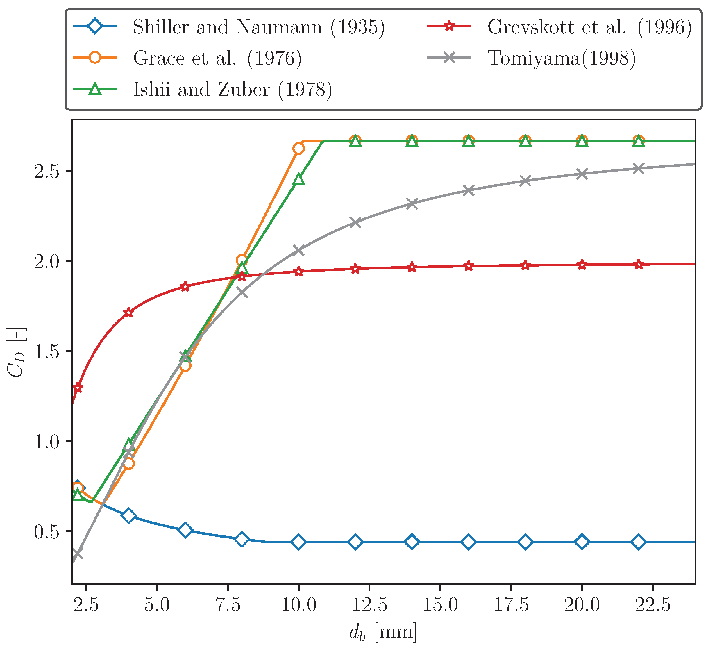
To properly solve the k-th equation, a feasible set of closure relations must be implemented to include all the possible interactions between primary and secondary phases, expressed in the form of momentum transfer per unit volume at the phase interface (Figure 5). Interfacial momentum forces are typically added as source terms in the momentum equation, and can be divided into drag and non-drag components.
The non-drag forces term comprises different physical mechanisms: lift, turbulent dispersion, wall lubrication, and virtual mass. Thus, the total interfacial force responsible for momentum exchange is provided by a linear combination of each individual force [12]. Indicating the continuous liquid phase with the subscript “L” and the dispersed gas phase with the subscript “G”, the source term in the momentum equation reads as follows:
M L G = M G L = F D , L G + F L , L G + F T D , L G + F D , W L G + F V M , L G
Figure 5. Schematic representation of the interphase forces acting on a bubble. Reprinted with permission from [13].
Fluids 08 00091 g005

3.2.1. Drag Force

The drag force reflects the resistance opposing the bubbles’ motion relative to the surrounding liquid. Due to rising upward motion through the continuous liquid phase, the dispersed phase particles are accelerated by buoyancy and slowed down by pressure effects and viscous friction at the interface. As the drag force accounts for such decelerating phenomenon, it is always applied in the opposite direction with respect to the bubble motion; therefore, it is flow region-dependent, and should be formulated with the inclusion of local flow parameters such as the relative slip velocity, particle diameter, and void fraction [12]:
F D , L G = 3 4 α G ρ L C D d b u G u L u G u L
In Equation (7), C D is the drag coefficient, which depends on the bubble size, shape, flow field, and contaminations. Therefore, it is a function of the relative bubble Reynolds number ( R e b ), Eötvös number ( E o ), and Morton number ( M o ) [12], defined as follows:
R e b = ρ L | u G u L | d b μ L
E o = g d b 2 σ ρ L ρ G
M o = g μ L 4 ρ L ρ G σ 3 ρ L 2
For spherical bubbles without deformation and fully contaminated systems, the functional form of the drag coefficient depends only on the bubble Reynolds number, as determined by Schiller and Naumann (1935) [14]. They modified the Stokes model, originally formulated only for creeping flows ( R e b < < 1 ), by adding a correction factor to extend its validity up to R e b = 1000 . A constant value of 0.44 was considered in order to extend the applicability of the model:
C D = 24 R e b 1 + 0.15 R e b 0.687 R e b 1000 0.44 R e b > 1000
This model is suitable only for small bubbles, and is commonly used in bubble columns operated in the homogeneous flow regime.
Similarly to Shiller and Naumann (1935) [14], White (1974) [15] proposed a drag coefficient correlation highlighting the dependency of the drag coefficient only on the bubble Reynolds number:
C D = 0.44 + 24 R e b + 6 1 + R e b
For deformed bubbles, the drag coefficient is affected by the Eötvös and Morton numbers. Grace et al. (1976) [16] were among the first to publish a drag law suitable for deformed bubbles:
C D = max min C D , ellipse , C D , cap , C D , sphere
where
C D , sphere = 24 R e b R e b < 0.01 24 R e b 1 + 0.15 R e b 0.687 R e b 0.01
C D , ellipse = 4 3 g d b U t 2 ρ L ρ G ρ L
C D , cap = 8 3
In Equation (15), the bubble terminal velocity ( U t ) is calculated as follows:
U t = μ L ρ L d b M o 0.149 ( J 0.857 )
where J is provided by the piecewise function
J = 0.94 H 0.757 2 < H 59.3 3.42 H 0.441 H > 59.3
and
H = 4 3 E o M o 0.149 μ L μ ref 0.14
In Equation (19), μ ref is set to 0.0009 kg/(m·s).
A model with the same functional form as Equation (13) was proposed by Ishii and Zuber (1979) [17], who distinguished different shape regimes and found the following:
C D , sphere = 24 R e b 1 + 0.1 R e b 0.75
C D , ellipse = 2 3 E o
C D , cap = 8 3
Except at high values of Eötvös number, this correlation agrees well with experimental results concerning the terminal velocity of bubbles rising in quiescent liquids.
Grevskott et al. (1996) [18] experimentally studied the drag coefficient considering the bubble size distribution in pure water by dividing the population of bubbles into small and large bubbles. Fitting the experimental data, they proposed the following drag coefficient correlation:
C D = 5.645 1.0 E o + 2.385 d b 2.0 mm 8 3 1 α G 2 d b < 2.0 mm
A popular correlation suitable for gas–liquid flows with a range of shapes was derived by Tomiyama et al. (1998) [19]. The proposed drag coefficient consists of three equations, respectively corresponding to pure, slightly contaminated, and fully contaminated systems:
C D = max min 16 R e b 1 + 0.15 R e b 0.687 , 48 R e b , 8 3 E o E o + 4
C D = max min 24 R e b 1 + 0.15 R e b 0.687 , 72 R e b , 8 3 E o E o + 4
C D = max 24 R e b 1 + 0.15 R e b 0.687 , 8 3 E o E o + 4
This drag correlation has a wide range of applicability ( 10 3 < R b < 10 6 and 10 2 < E o < 10 3 ) and holds for spherical as well as deformed bubbles.
Zhang et al. (2006) [20] derived a simple relation that provides results comparable to other models when the bubble diameter is in the range between 4 mm and 10 mm, for which the rising velocity is weakly dependent on the bubble diameter:
C D = 2 3 E o
Recently, Dijkhuizen et al. (2010) [21] used a DNS front-tracking technique to derive a correlation valid for both spherical and deformed bubbles:
C D = C D 2 R e b + C D 2 ( E o )
where
C D R e b = 16 R e b 1 + R e b 8 + 0.5 R e b + 3.315 R e b 0.5
C D ( E o ) = 4 E o 9.5 + E o
The proposed drag closure matches very well with experimental data for ultra-pure liquids (water/glycerine mixture). A comparison between the different drag coefficient correlations is presented in Figure 6.

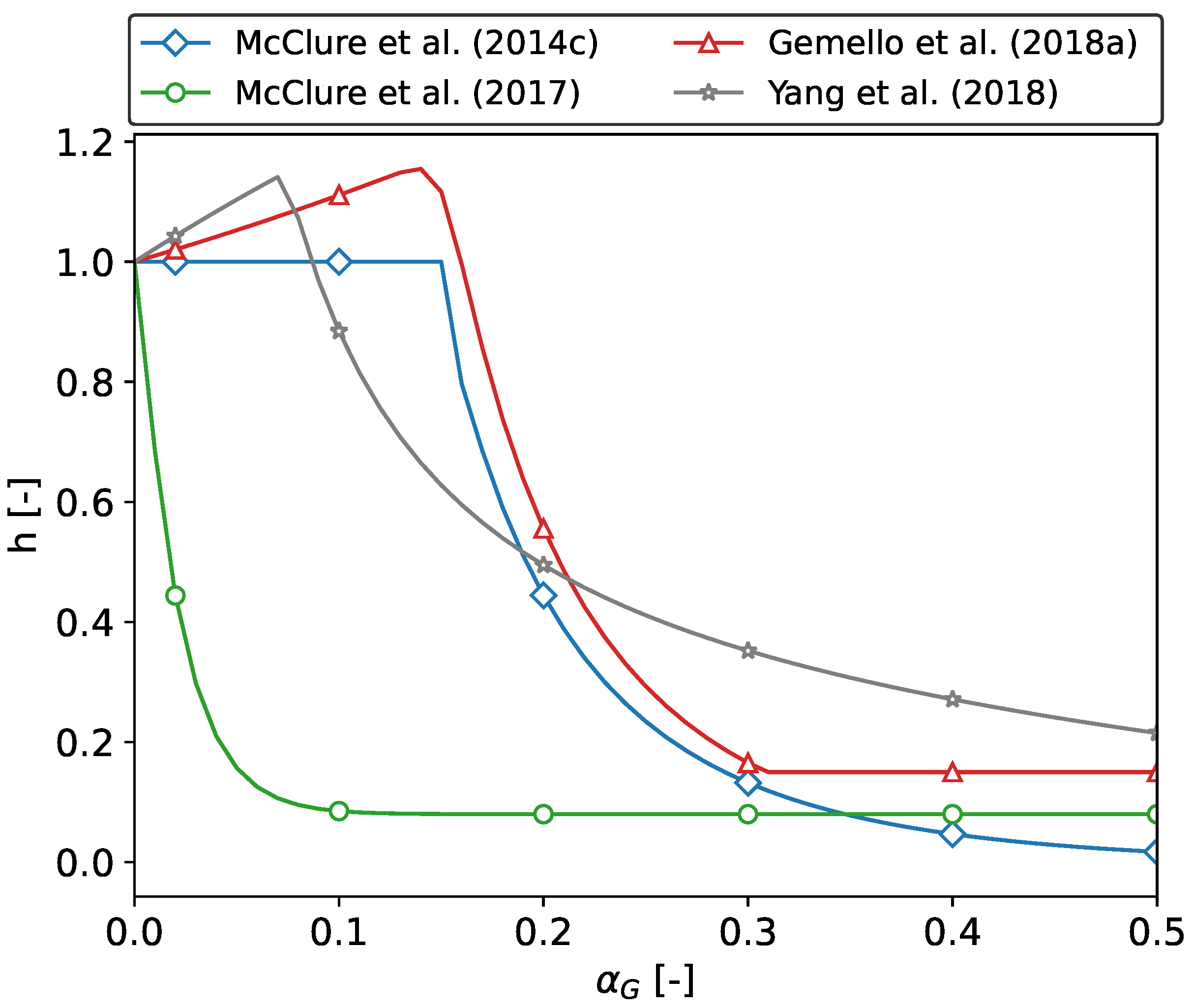
3.2.2. Swarm Factor Definitions
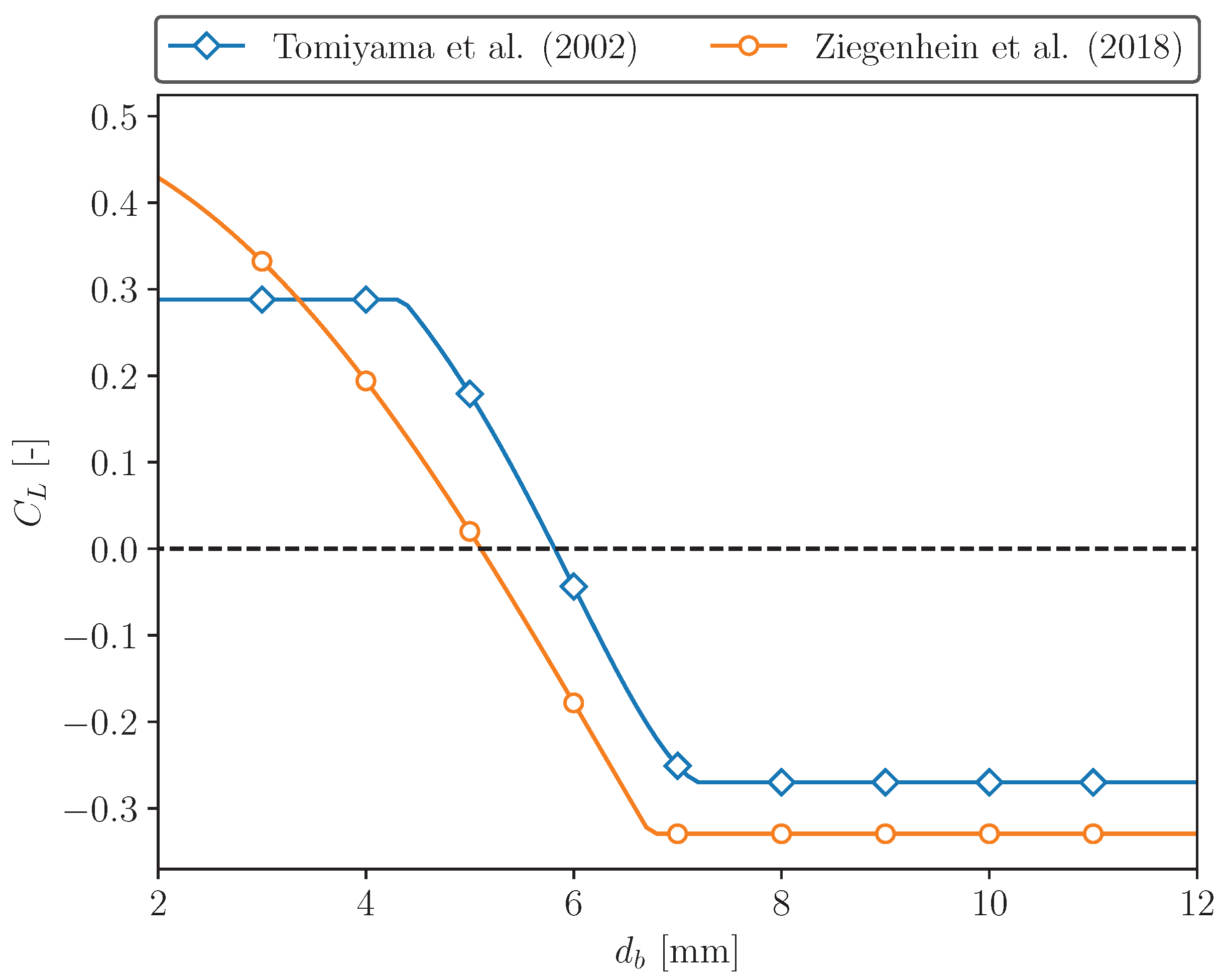
The drag coefficient correlations presented in Section 3.2.1 apply to isolated bubbles rising in initially quiescent liquids, and can only be used for low gas volume fractions. In the case of high gas volume fractions, as is common in industrial bubble columns with high superficial gas velocity, bubbles are very close to each other, resulting in a crowding effect in which bubbles travel through the column in swarms. The bubble boundary layers interact, changing the interphase momentum exchange and, importantly, the drag force. For this reason, a correction factor (h) should be applied to the drag coefficient for isolated bubbles
h = C D C D
where C D is the actual drag coefficient and C D is the drag coefficient for an isolated bubble.
Several authors have investigated the impact of bubble–bubble interactions on the drag coefficient. The first approach was proposed by Bridge et al. (1964) [22] and Wallis (1969) [23]:
h = 1 1 α G 2 n
for which Bridge et al. (1964) [22] selected n = 1.39 and Wallis (1969) selected [23] n = 1 .
Ishii and Zuber (1979) [17] investigated the drag force over a broad range of gas volume fractions and Reynolds numbers, establishing the following relation based on a large sample of experimental data:
h = 1 1 α G
Rusche and Issa (2000) [24] proposed a swarm factor correlation for oblate bubbles, validated for a local volume fraction α G 0.45 and 27 R e b 960 :
h = exp 3.64 α G + α G 0.4864
Roghair et al. (2011) [25], using a DNS front-tracking model, derived a drag-modification term that can be applied for high Reynolds numbers and oblate bubbles in the range α G < 0.45 , 150 R b 1200 , 1 E o 5 , 4 × 10 12 M o 2 × 10 9 :
h = 1 + 18 α G E o 1 α G
Buffo et al. (2016) [26] developed a straightforward power law equation to account for the crowding effect of bubbles based on many investigations into fluidized beds and liquid–liquid systems:
h = 1 α G C A α G 0.8 1 α G > 0.8
The authors concluded from a sensitivity analysis that a value of C A = 1.3 provides the best agreement with experimental data.
The swarm factor correlations discussed above hinder the rising velocity of the bubbles, thereby increasing the drag coefficient of isolated bubbles at high gas volume fractions. They are reported in Figure 7 and compared with the Simmonet et al. (2008) [27] model; while reasonable agreement is found at low gas volume fractions, the predictions diverge strongly at high volume fractions. The correction factor proposed by Simmonet et al. (2008) [27] differs from the other models in highlighting the presence of a critical value of the gas volume fraction at 0.15. Below this value, the rising velocity of the bubbles decreases with increasing void fraction; on the contrary, beyond the critical value the wake acceleration effect of large bubbles is predominant, causing an increase in the bubbles’ rising velocity and a consequent reduction in the swarm factor, which decays rapidly to zero. For local void fractions less than 0.30 and air–water pure systems, the correlation of Simonnet et al. (2008) [27] reads as follows:
h = 1 α G 1 α G m + 4.8 α G 1 α G m 2 / m
where m is an adjustable coefficient. Simonnet et al. (2008) [27] set m = 25 , as this showed good agreement with their experimental data.
McClure et al. (2014c) [28] suggested that no hindering effect should be taken into account for bubbles larger than 7 mm, and modified the correlation of Simonnet et al. (2008) [27] accordingly:
h = min h , 1 h > 1 0.8 h h < 1
where h is the original swarm factor of Simonnet et al. (2008) [27].
Performing a new experimental study, McClure et al. (2017) [29] criticized their previous model and observed that the drag correction factor is a function of both the bubble size distribution and the local gas volume fraction. Thus, they proposed a new empirical correlation valid for α G > 0.25 :
h = min 1 α G n + b , 1
where n and b are model constants calculated with least-square fitting of experimental data. The authors suggested n = 50, while b depends on the gas sparger design (for example, a value of 0.20 was found in the case of a perforated plate distributor with a 0.5 mm hole diameter, while a value of 0.08 was found in the case of a perforated plate with a 3 mm hole diameter).
Gemello et al. (2018a) [30] modified the correlation proposed by Simonnet et al. (2008) [27] (validated for α G < 0.3 ) to obtain a swarm factor feasible for a wide range of operating conditions. In particular, they noted that the decrease in the swarm factor proposed by Simonnet et al. (2008) [27] is too strong for high volume fractions; thus, they added a minimum asymptotic value ( h min ) towards which h should tend at high void fractions:
h = max 1 α G 1 α G 25 + 4.8 α G 1 α G 25 2 / 25 , h min
The authors suggested h min = 0.5 for industrial scaling-up purposes.
Yang et al. (2018) [31] formulated a drag modification relation for bubble swarms that accounts for both the hindering effect of small bubbles and the wake accelerating effect of large bubbles. To model both phenomena, the resulting swarm factor was calculated using the product of two corrective terms:
h = k b , large · k b , small
k b , large = 1 max 1.90 α g f b , large
k b , small = 1 α G , small 1 + 22 α G , small Eo + 0.4
where f b , large is the fraction of large bubbles and α G , small = α G 1 f b , large . From this model equation, it is possible to observe that an increasing void fraction means that the drag correction factor increases to a maximum and then decreases. Drag correction factors that reduce the drag force in bubble swarms are presented in Figure 8.

3.2.3. Lift Force

A bubble moving through a shear fluid is subjected to a force perpendicular to its motion. This force results from the action of pressure and stress on the surface of the bubble. The corresponding momentum source is
F L , L G = C L ρ L α G u G u L × × u L ,
where C L is the lift coefficient. Experimental and numerical studies show that the coefficient is positive for small bubbles and negative for large bubbles. Consequently, the lift force direction depends on the bubble size and shape. For small bubbles, the lift force acts in the direction of decreasing liquid velocity, which in the case of batch or co-current mode is toward the pipe wall. Conversely, when large bubbles are considered, a force assimilated to the lift force pushes the bubbles towards the centre of the column. In other words, sign reversal of the lift force is observed for bubbles with a diameter larger than a critical value ( d c r ). Smaller bubbles (those with a diameter lower than the critical threshold) tend to move towards the wall, whereas larger bubbles (those for which d b > d c r ) are pushed towards the vessel centre.
Tomiyama et al. (2002b) [32] studied the motion of bubbles in a glycerol–water solution, deriving the following correlation for the lift coefficient:
C L = min 0.288 tanh 0.121 R e b , f E o E o 4 f E o 4 < E o 10 0.27 E o > 10
where
f E o = 0.00105 E o 3 0.0159 E o 2 0.0204 E o + 0.474 ;
here, E o is the modified Eötvös number calculated considering the maximum horizontal dimension (major axis) of the bubble ( d ), provided by the empirical correlation for the aspect ratio (E) proposed by Wellek et al. (1966) [33] for contaminated flows:
E o = g ρ L ρ g d 2 σ
d = d e q 1 E 1 / 3 = d e q 1 + 0.163 E o 0.757 3
where d e q is the equivalent spherical diameter of the bubble.
This correlation applies to larger-scale deformable bubbles in the ellipsoidal and spherical cap regimes. The experimental conditions under which Equation (45) was derived were limited to the ranges of 5.5 l o g 10 ( M o ) 2.8 and 1.39 E o 5.84 . Air–water systems at normal conditions usually have M o = 2.63 × 10 11 ( l o g 10 ( M o ) = 10.55 ), which is quite different from the conditions at which the above correlation was derived; nevertheless, good results have been reported for this case. When coupled with that of Wellek et al. (1966) [33] for the calculation of d , the correlation predicts that the change in sign of the lift coefficient occurs at d b = 5.8 mm.
However, Ziegenhein and Lucas (2019) [34] pointed out that the correlation of Wellek et al. (1966) [33] is not suitable for purified air–water systems and leads to an over-prediction of the major axis of an elliptic bubble. Besagni et al. (2016) [35] studied the size distribution and shapes of bubbles in an annular gap bubble column and reached the same conclusion. Correct estimation of the critical diameter is essential in CFD modelling, as it allows the bubble population to be divided into a small group and large group, permitting consideration of the poly-disperse nature of the flow in which bubbles of different sizes move in different directions.
To overcome this limitation, Ziegenhein et al. (2018) [36] suggested a quadratic fit correlation for the lift force as a function of the modified Eötv s .. number and bubble Reynolds number:
C L = 0.002 E o 2 0.1 E o + 0.5 E o 10.5 0.3295 E o > 10.5
In their model, the correlation for the bubble major axis is modified based on experimental observation of bubble shapes in six column configurations:
d = d e q 1 + 0.65 E o 0.35 3
The Ziegenhein et al. (2018) [36] correlations results in a critical diameter of about 5.3 mm, which is lower than that obtained with the Wellek et al. (1966) [33] relation. Figure 9 shows a comparison between the Tomiyama et al. (2002) [32] and the Ziegenhein et al. (2018) [36] lift models.
To conclude, Behzadi et al. (2004) [37] proposed a model highlighting that the lift coefficient cannot be independent of the local gas void fraction. After fitting their experimental observations, they proposed the following correlation:
C L = 6.51 × 10 4 α G 1.2
It should be pointed out that this simple correlation does not consider the change of sign of the lift coefficient (i.e., C L does not depend on E o ) and, due to the power law formulation, the coefficient tends to infinity for α G 0 . This is avoided by limiting Cl by a finite value, which is taken as 0.25 [37].

3.2.4. Turbulent Dispersion Force

The turbulent dispersion force accounts for the fluctuations in the liquid velocity that affect the dispersed phase by scattering it. The turbulent eddies redistribute the bubbles in the lateral direction from regions with high concentration to regions with low concentrations. The effect of the turbulent dispersion force is evident in the gas fraction profiles, as it modulates peaks of small bubbles near the wall pipe and spreads out large bubbles.
The modelling of the turbulent dispersion force is expressed as a force proportional to the void fraction gradient. Simonin and Viollet (1990) [38] proposed the following model for the turbulent dispersion force:
F T D , L G = C T D k L G D t , L G σ L G α L α L α G α G
In analogy to the molecular diffusion, σ T D is the Schmidt number (a value of σ T D = 0.9 is typically used) and C T D is the turbulent dispersion coefficient, while k L G and D t , L G are the mixture’s turbulent kinetic energy and the liquid dispersion scalar, respectively.
Burns et al. (2004) [39] derived an explicit formulation for the turbulent dispersion force by using Favre averaging on the drag force:
F T D , L G = 3 4 C T D α L 1 α L C D d b u G u L μ L turb σ T D α L α L α G α G
This model estimates the dispersion scalar of the Simonin and Viollet (1990) [38] model with the liquid turbulent viscosity μ L turb .
An alternative formulation is the one proposed by Lopez De Bertodano et al. (2004) [40]:
F T D , L G = ρ L 1 S t ( 1 + S t ) u L u L ¯ · α G
where S t is the Stokes number and u L u L ¯ represents the normal Reynolds stresses.

3.2.5. Wall Lubrication Force

The wall lubrication force is caused by the surface tension and prevents the bubbles from touching the walls, ensuring zero void fraction (as found experimentally) near the vertical walls.
The wall lubrication force has the general form
F W L , L G = 2 d B C W L ρ L α G ( u G u L | | | 2 y ^
where ( u G u L ) | | is the relative velocity component parallel to the wall, y ^ is the unit normal to the wall pointing into the fluid, and C W L is the wall lubrication coefficient.
Different expressions for C W L have been proposed in the literature. The relation proposed by Antal et al. (1991) [41] states that
C W L = max 0 , C w 1 d b + C w 2 y w
With C w 1 and C w 2 being two non-dimensional coefficients. The Antal et al. (1991) [41] model is applicable only if the condition y w 5 d b is respected; thus, it is only active on a sufficiently fine mesh. Tomiyama et al. (1995) [42], studying bubble trajectories in a glycerol–water solution, proposed a different function for the wall lubrication coefficient by considering an additional dependence on the Eötvös number and pipe diameter (D):
C W L = C w d b 2 1 y w 2 1 D y w 2
C w = 0.47 E o < 1 e 0.933 E o + 0.179 1 E o 5 0.00599 E o 0.0187 5 < E o 33 0.179 33 E o
Although the Tomiyama (1995) [42] model has proven superior to the Antal et al. (1991) [41] model, it is restricted to flows in pipe geometries.
Hosokawa et al. (2002) [43] reviewed the experimental results of Tomiyama (1995) [42] and obtained the following functional form for C W L :
C W L = C w d b 2 y w
Here, the coefficient C w depends on the Eötvös number and the phase-relative Reynolds number ( R e b ), as indicated below:
C w = max 7 R e b 1.9 , 0.0217 E o
The Hosokawa et al. (2002) [43] model often shows better agreement with experimental data in both vertical and inclined bubbly flow systems.
Later, Frank et al. (2005) [44] proposed a generalized formulation for the wall lubrication coefficient:
C W L = C w ( Eo ) · max 0 , 1 C W D · 1 y w C W C d b y w · y w C W C d b p 1
where C W C and C W D are the cut-off and the damping coefficient, respectively. The Eötvös number coefficient C w is provided by Equation (58). From numerical simulations, the authors found that good agreement with the experimental data was obtained for C W C = 10 , C W D = 6.8 , and p = 1.7 .
Figure 10 shows the influence of the above described non-drag forces on the numerical prediction of the local void fraction profile [45].

3.2.6. Virtual Mass Force

The virtual mass force arises from the acceleration of an immersed moving object relative to the surrounding fluid. This effect is significant when the continuous phase density is much higher than that of the dispersed phase.
F V M , L G = C V M α G ρ L D G u G D t D L u L D t
Here, D j / D t , D k / D t denote the total derivative with respect to time for the indicated phase. As reported by Tabib et al. (2008) [46], the contribution of virtual mass is negligible for large-diameter bubble columns ( D > 0.15 m). A common practice is to set a constant value C V M = 0.5 , which has been obtained experimentally for isolated spherical bubbles, as the virtual mass coefficient.

3.3. Population Balance Modelling

Most of the interfacial correlations defined in Section 3.2 require the equivalent diameter of the bubbles as an input; in this regard, three approaches can be used to model the dispersed phase: (1) the mono-dispersed model, (2) the homogeneous Multiple Size Group model (MUSIG), and (3) the inhomogeneous Multiple Size Group model (iMUSIG). The mono-dispersed approximation considers two separate continuity and momentum equations for the gas and liquid phases. The MUSIG model applies to poly-dispersed systems, with the bubble population divided into two groups with different sizes. This model solves a separate continuity equation for each size group and a single momentum equation for all sizes together. Conversely, the iMUSIG model considers several velocity groups and solves a separate momentum equation for each [47].
An uncertainty in bubble column design and scale-up arises from a lack of understanding of the phenomena governing bubble size distribution (BSD), and consequently the column fluid dynamics and interfacial area. Bubble size distributions depend on many phenomena occurring in the bubble column, including the balance between the coalescence and breakup rate, the pressure change, and the gas–liquid mass transfer. In particular, the bubble size distribution mainly results from the coalescence and breakup phenomena occurring in the bubble column.
Consequently, the dispersed phase characteristic properties vary in time and space, meaning that a constant bubble size distribution represents a strong assumption. To account for the changes in the particle population, a balance equation can be included in addition to the mass, momentum, and energy balances within the contest of MUSIG and iMUSIG models. This concept is referred to as the Population Balance Model (PBM).
A population balance model can be described by a transport equation reflecting particles entering or leaving a control volume via several mechanisms. The bubble number density function, called the population balance equation (PBE), reads [48]:
t n x , V b , t + z n x , V b , t u b x , V b + V b n x , V b , t t V b x , V b = S x , V b , t
where n x , V b , t is the bubble density distribution function that specifies the probable number density of bubbles at a given time (t) in the spatial range ( d ( x ) ) about a position x for a bubble volume between V b and V b + d ( V b ) at time t. Finally, S x , V b , t is the following source term:
S x , V b , t = S b + S c + S p h + S p + S m + S r
where S b , S c , S p h , S p , S m , and S r are the bubble source/sink terms due to breakup, coalescence, phase change, pressure change, mass transfer, and reaction, respectively.
The breakup source term ( S b ) reads
S b = v m ( V b ) β ( V b , V b ) g ( V ) n ( V b , t ) g ( V b ) n ( V b , t )
where the first term is the birth rate of bubbles of volume V b due to the breakup of bubbles with volumes larger than V b , the second term is the death rate of bubbles of volume V b due to breakup, m ( V b ) is the mean number of daughter bubbles produced by the breakup of a parent bubble with volume V b , g ( V b ) is the breakage frequency (the fraction of particles of volume V b breaking per unit time), and β ( V b , V b ) denotes the daughter distribution factor of a particle of volume V b breaking from a parent bubble of volume V b .
The coalescence source term ( S c ) reads
S c = 1 2 0 v Γ V b V b , V b n V b V b , t n V b , t d V b n V b , t 0 Γ V b , V b n V b , t d V b
where the first term is the birth rate of bubbles of volume V b due to the coalescence of bubbles of volume V b V b and V b , the second term is the death rate of bubbles of volume V b due to coalescence with others bubbles, and Γ ( V b , V b ) is the coalescence rate between bubbles of volume V b and V b .
Neglecting the interfacial mass transfer, the reaction contribution, the phase variations, and the changes due to pressure gradients, the coalescence and breakup phenomena are the only items of interest. Considering a steady state, it follows that
u b , i n i z = S i ( x , V b ) = S c + S b
Which can be rewritten in terms of bubble diameter as
u b , i n i z = S i ( x , d b ) = S c + S b
where S c and S b are determined by modelling the breakup and coalescence rates.

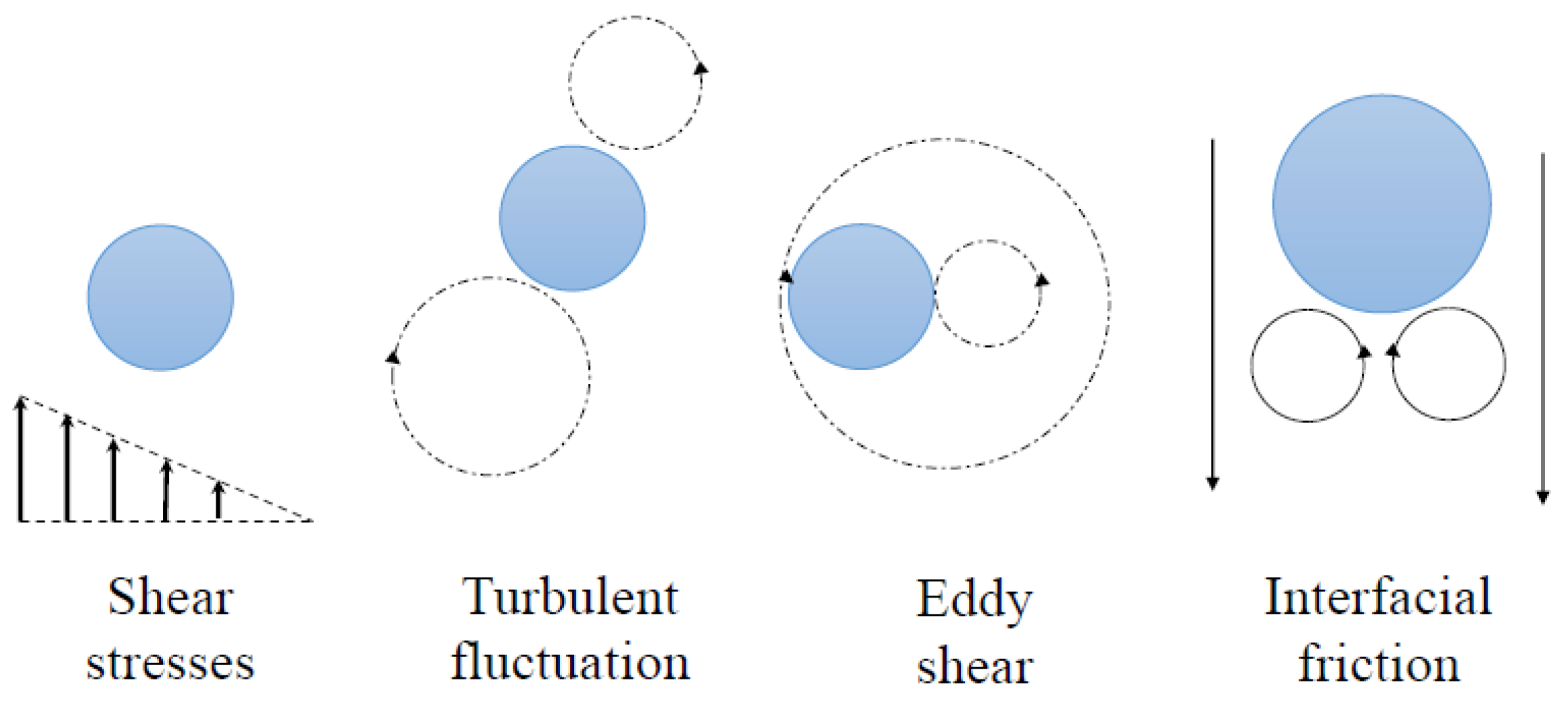
3.3.1. Bubble Breakup Phenomena Modelling

The breakup of fluid particles in the dispersed phase depends on the hydrodynamics of the continuous phase and interface interactions. The phenomenon of rupture can be expressed as a balance between two opposite effects, namely, the external stresses of the continuous phase, which attempt to destroy the bubble, and the surface stress of the particle plus the viscous stress of the fluid inside it, which opposes the deformation of the bubble. Therefore, breakage is caused by the hydrodynamic conditions in the surrounding liquid and the properties the bubble itself [49].
The breakage mechanism can be classified into four categories [49] (Figure 11):
  • Turbulent fluctuations and collisions, in which breakage is mainly caused by turbulent pressure fluctuations along the surface or by particle-eddy collisions. The dominant external force is the dynamic pressure difference around the bubble, meaning that the breakage process can be studied as the balance between the dynamic pressure and surface stresses.
  • Viscous shear stresses, which cause a velocity gradient around the interface that can deform or break the bubble. In addition, wake effects may be responsible for the formation of shear stresses. Breakage can be modeled as the balance between external viscous stresses and surface tension forces as expressed by means of the capillary number C a .
  • Shearing-off processes, which occur when small bubbles are sheared off from a large bubble through erosive breakage.
  • Interfacial instabilities, which arise in the absence of a continuous phase net flow. If a significant density difference is present, as in the case of a light liquid accelerated into a heavy fluid, Rayleigh–Taylor instabilities are found; on the other hand, if the density ratio is close to unity Kelvin–Helmholtz instabilities exist.
In general, the most common causes of breakage are associated with turbulent fluctuations and the other mechanisms are often neglected.
Modelling of breakup phenomena requires definition of the breakage frequency (g) and daughter size distribution function. Applicable breakup models for bubble columns are reported in Table 2.

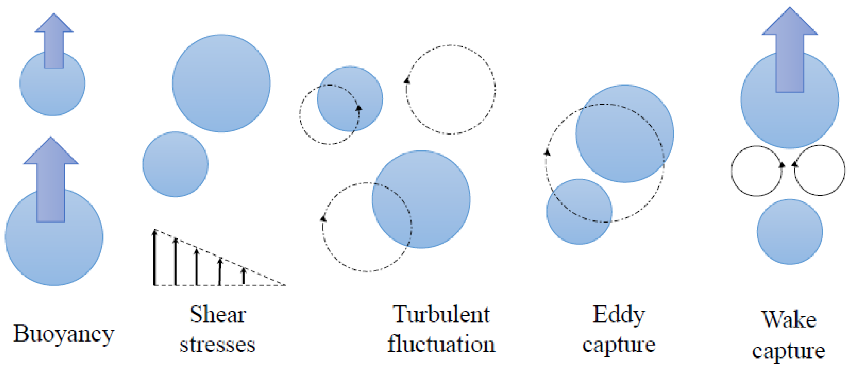
3.3.2. Bubble Coalescence Phenomena Modelling

According to Chesters (1991) [56], the coalescence process is more complex than breakup, as it involves interactions of bubbles with the surrounding liquid phase as well as those between bubbles themselves when they are brought into contact by the external flow or body forces [48]. Coalescence can be modelled by using empirical or physical models. The former are much easier to implement in CFD simulations, as they typically take the form of power law functions with adjustable coefficients. However, because these models depend on the experimental facility geometrical aspects, the results cannot be extended to other setups. The latter models attempt to describe the underlying physics of the phenomenon by identifying specific physical parameters capable of detailing the bubble collision mechanism. In this approach, the coalescence kernel is determined as the product of the collision frequency ( Γ ( d b , d b )) and coalescence efficiency λ ( d b , d b ):
Γ ( d b , i , d b , j ) = h ( d b , i , d b , j ) λ ( d b , i , d b , j )
where d b , i and d b , j are the diameters of the two colliding bubbles.
The collision frequency represents the number of collisions between bubbles per unit of time. For a turbulent bubbly flow, there are five mechanisms of collision (Figure 12):
  • Turbulence-induced collisions occur as a result of the random motion of bubbles caused by turbulent fluctuations.
  • Viscous shear-induced collisions are generated by global liquid velocity gradients, meaning that bubbles in a location of high liquid velocity may collide with those in a region of low liquid velocity.
  • Eddy-capture, in which collision events are produced by the shear rate of the flow in the turbulent eddy.
  • Bouyancy-induced collisions, in which collisions may occur because bubbles of different size have different rising velocities.
  • Wake entrainment collisions, which may result when bubbles are accelerated by the wake region behind a large spherical-cap bubble.
Thus, the overall rate of collision events is determined by the sum of the effects of all the listed mechanisms. Typically, only turbulence-induced collisions are assumed to be predominant. The others are frequently insignificant except at very high superficial gas velocities (where, for example, wake entrainment effects cannot be ignored due to the formation of large spherical-cap bubbles).
Bubble collisions do not always lead to coalescence, as bubbles may bounce off each other or separate after the collision. Hence, the efficiency term ( h ( d b , d b ) ) is introduced in the definition of the coalescence kernel. Three models for calculation of the coalescence efficiency have been introduced:
  • Film drainage model: first proposed by Shinnar and Church (1960) [57], this is a widely used model of coalescence efficiency. When two bubbles collide, a thin liquid film is trapped between their surfaces and is progressively drained. If the contact time is sufficiently high, the liquid film reaches a minimum thickness, then ruptures, causing coalescence.
  • Energy model: first proposed by Howarth (1964) [58], this model is based on the concept of collision energy, in which a higher collision energy indicating a higher probability of coalescence.
  • Critical approach velocity model: in this model, collisions result in coalescence phenomena if the approach velocity of the bubbles exceeds a certain critical value; otherwise, they bump into or bounce off of each other, and do not coalesce.
Several different coalescence frequency and efficiency models have been proposed; the ones most commonly used in bubble column simulations are presented in Table 3.

3.3.3. Solution Methods

Many numerical schemes are available in the literature to solve the population balance in Equation (63). These can be classified into four main categories:
  • Class (or Sectional) Method (CM): the internal coordinate domain is divided into a finite number of intervals (or bins), transforming the population balance equation into a set of balance equations in the physical domain. Any coalescence and/or breakup event is accompanied by the migration of particles from one class to the adjoining classes. The advantages of this method are its robust numerics and that it computes the Particle Size Distribution directly [62].
  • Monte Carlo Method: this method solves the population balance equation based on the statistical ensemble approach, accurately tracking particulate changes in a multidimensional system. Nevertheless, the method accuracy strongly depends on the number of simulation particles, and requires an extensive computational time to track large numbers of particles. This makes the Monte Carlo method poorly compatible with the conceptual framework of Computational Fluid Dynamics [47].
  • Standard Method of Moments (SMM): the population balance equation is turned into a set of transport equations for the moment of the particle size distribution. The primary advantage is numerical economy, as it is sufficient to solve a limited number of moment equations. Mathematically, the transformation from the space of particulate size distribution to the space of moments is extremely rigorous, and fractional moments, representing the Sauter mean diameter of the bubbles, present a serious closure problem [47]. This closure constraint can be overcome by resorting to a Quadrature Method of Moments (QMOM) approach.
  • Quadrature Method of Moments (QMOM): first suggested by McGraw (1997) [63] for modelling aerosol and coagulation problems, QMOM was later applied by Marchisio et al. (2003) [64] for solving the population balance equation, becoming an attractive alternative. Compared to the SMM method, this approach solves only the transport equations of the low-order moments; however, it is able to overcome the closure problem of the SMM method [64]. With the QMOM, the integral terms in the momentum transport equations are approximated by employing an N-node Gaussian quadrature formula. This quadrature approximation requires knowledge of N weights ( ω i ) and N nodes of abscissas L i , and determines a sequence of polynomials orthogonal to the unknown number density function. The functional form (for a univariate problem with ϕ as internal coordinate) reads as follows:
    0 f ( ϕ ) n ( ϕ ) d ϕ i = 1 N f L i w i
    where the weights ( ω i ) and abscissas ( L i ) are determined through the Product–Difference (PD) algorithm from the lower-order moments [64]. When the weights and abscissas are known, the source term due to coalescence and breakup can be calculated and the transport equation for moments can be solved. Finally, starting from the moments of the distribution, it is possible to solve the inverse problem of reconstructing the bubble size distribution [62].
    When dealing with a multivariate population balance equation, for which the product–difference algorithm can not be applied, other extensions of QMOM are available, such as the Conditional Quadrature Method of Moments (CQMOM) or the Direct Quadrature Methods of Moments (DQMOM). In DQMOM, the transport equations are directly solved for the weights and nodes of the quadrature approximation, whereas CQMOM represents the multivariate extension of QMOM. Moreover, in CQMOM closure is achieved by means of multivariate quadrature approximation, and the transport equations for the moments of the distributions are solved [65].
From the above discussion, it is clear that for univariate problems (which is the case for bubble columns when the mass transfer is not modelled) the class method and quadrature method of moments are the only viable candidates for solving the population balance equation.
In the class method, a high number of bubble classes (i.e., 12–18) are required to describe the evolution of the particle population accurately, which incurs high computational costs. On the contrary, in the quadrature method of moments approach it is sufficient to solve a limited number of moments (i.e., 4–8), yielding a reduction in the dimensionality of the problem compared to the class method, in turn leading to lower computational costs [62].

3.4. Turbulence Modelling

Turbulence modelling in bubbly flows has predominant importance due to its significant influence on the local distribution of the dispersed phase and in determining the coalescence and breakage phenomena. The description of the effects of turbulent fluctuations of velocities and other scalar quantities in multiphase simulations is complex, as the number of terms to be modelled in the momentum equations is larger compared to the case of single-phase flows. Moreover, turbulent mixing occurs in bubble columns over a wide range of length and time scales [66]; the largest turbulent scales are of the same order of magnitude as the characteristic scales of the mean flow, and depend on the geometry and boundary conditions, the smaller turbulence scales depend on bubble dynamics and are proportional to the bubble diameter, and the smallest scales are associated with the Kolgomorov scale and are responsible for the dissipation of the turbulent kinetic energy. Considering the importance of turbulence, a variety of numerical methods have been developed to address this issue, which can be grouped into the three following categories: (1) Reynolds-Averaged Navier–Stokes (RANS) models; (2) Large Eddy Simulation (LES); and (3) Direct Numerical Simulation (DNS).
In RANS turbulence models, attention is focused on the mean flow characteristics; the instantaneous flow equations are time-averaged through a Reynolds decomposition approach applied to both pressure and velocity components in the continuity and momentum equations. Six extra terms involving the products of fluctuating velocity components, called Reynolds stresses, appear after performing this time-averaging process. Appropriate closure relations, namely, k ε and k ω , are required to solve the system of mean flow equations, making use of the Boussinesq hypothesis based on the assumption of isotropic turbulence. This approximation considers the Reynolds stresses proportional to the mean rates of deformation of the fluid elements. The generic component of the viscous stress tensor τ for a Newtonian fluid results in the following expression:
τ i j = ρ u ı u j ¯ = μ t U i x j + U j x i 2 3 ρ k δ i j
where δ i j is the Kronecker delta and k = 1 2 u 2 ¯ + v 2 ¯ + w 2 ¯ is the turbulent kinetic energy per unit mass. The first term on the right-hand side of Equation (71) contains the turbulent eddy viscosity μ k . For k ε models, the turbulent viscosity is provided by
μ t = ρ C μ k 2 ε
where C μ is a dimensionless constant, often taken as 0.09. With RANS models, the computational resources needed for reasonably accurate flow simulations are modest, making them the mainstay of many engineering flow calculations. Multiphase turbulence RANS models are derived directly from their single phase equivalents.
The isotropic turbulence assumption for the core of the flow in RANS models is not strictly satisfied for bubble columns, as the velocity fluctuations in the gravity direction are normally twice those in the other directions [67]. As a result, the turbulence generated by the rising bubbles is mainly anisotropic. RANS models fail to exactly represent the directional effects of the Reynolds stress field; the Reynolds Stress Model (RSM) can be used to address these problems adequately, as it incorporates anisotropy by solving the transport equation of each Reynolds stress component. This increases the computer storage and run time, and as a result has found little success in the simulation of bubbly flows. Nonetheless, RSM seems a promising tool to provide more realistic numerical prediction of turbulence quantities that can be used as inputs in bubble coalescence and breakage models [68,69].
A further option is the use of Large Eddy Simulation (LES), an approach that uses an unsteady flow computation to resolve only the turbulent structures that have a length scale larger than a certain cutoff, then describes the smaller eddies and their effects on the larger scales by means of Sub-Grid-Scale (SGS) models. By resolving only large portions of the turbulent motion, LES appears to be more suitable for accounting for anisotropic structures in bubble columns; however, this comes at the cost of a much larger volume of calculations compared to RANS methods. Another issue is selection of the proper mesh size, which when using LES should be bounded within a certain range in order to obtain a correct filter cutoff width; a very dense grid is commonly required. Thus, LES may be unable to consistently represent the correct sub-grid-scale stress for various flow situation [46].
DNS does not include any turbulence modelling, and directly resolves the instantaneous Navier–Stokes equations while considering all turbulence scales of motion and even the fastest fluctuations. Unfortunately, its enormous computational and memory storage requirements make its applicability to industrial-scale reactors unfeasible.

Bubble-Induced Turbulence

Experimental observations have found that the sources of the bulk liquid turbulence can be divided into two categories, namely, (1) Shear-Induced Turbulence (SIT) and (2) Bubble-Induced Turbulence (BIT). The former is independent of the bubble size, whereas the presence of gaseous bubbles generates the latter. When a bubble rises in a pool of liquid in a turbulent flow regime, a portion of its pressure energy is converted into liquid phase turbulence, then into internal energy at the level of the Kolmogorov scale [70].
Within the context of the RANS k ε and k ω models, it is common practice to account for the influence of the dispersed phase on the liquid phase turbulence by adding extra source terms ( S k , L , S ε , L , or S ω , L ) to the transport equations for the turbulence quantities. A plausible approximation is that all energy lost by bubbles due to the drag force is converted to turbulent kinetic energy (k) in the wake of the bubble [71]. Hence, the k-source becomes
S k , L = F D , L G u G u L
The ε -equation source term is obtained by dividing the k-equation source term by a characteristic time scale ( τ p ):
S ε , L = C ε B S k , L τ p
The ε -source term can be transformed into into an equivalent ω -source term as follows:
S ω , L = 1 C μ k L S ε , L ω L k L S k , L
Modelling of the time scale ( τ p ) proceeds largely based on dimensional analysis [71]. The time scale factors commonly used in numerical simulation of bubble columns are presented in Table 4.
Unlike the model presented in Table 4, Sato and Sekoguchi (1975) [77] did not explicitly add source terms in the turbulence transport equations, rather, they tried to incorporate the effects of bubble-induced turbulence in the turbulent viscosity, proposing the relation
ν L = C μ k L 2 ε L + 0.6 α G d b u G u L .

4. Literature Survey

Table 5, Table 6, Table 7 and Table 8 collect different studies regarding CFD simulations of bubble columns validated with experimental data; Table 5, Table 6 and Table 7 refer to the operating conditions, physical settings, and numerical settings, respectively. Conversely, Table 8 focuses on model performance. To derive a consistent comparison between different studies, the values in Table 8 have been computed by extracting published values using a consistent procedure. The CFD accuracy is assessed by computing the relative error ( δ ) between numerical ( ω CFD ) and experimental ( ω EXP ) data, as follows:
δ = ω CFD ω Exp ω Exp
When local validation wis performed with N local quantities (i.e., local void fraction profile and local liquid velocity profile), the error ( δ ) is computed as follows:
δ = 1 N i = 1 N ω CFD , i ω Exp , i ω Exp , i
Pfleger and Becker (2001) [74] performed 3D transient simulations of a 0.288-m inner diameter bubble column operating in the homogeneous flow regime using a mono-dispersed approach. Concerning the interfacial forces, they considered only the drag force with a constant drag coefficient C D = 0.44 . The standard k ε model was used for turbulence in the liquid phase. Their main aim was to study the effect of BIT on the correctness of CFD predictions. The local liquid velocity and local void fraction showed the positive impact of the BIT model, with δ = 30.29 % ( δ = 51.75 % without BIT) and δ = 4.21 % ( δ = 11.14 % without BIT), respectively. The simulation results, including BIT or not, were found to over-predict the global gas holdup, which the authors attributed to the simplified gas inlet modelling.
Chen et al. (2005) [78] carried out 2D axisymmetric transient simulations in a 0.19-m inner diameter bubble column operating in the heterogeneous flow regime. The main focus was studying the influence of different coalescence and breakup models. In particular, they compared the coalescence efficiency of Prince and Blanch (1990) [50], Chesters (1991) [60], and Luo (1993) [61] and the breakup kernels of Luo and Svendsen (1996) [51] and Martinez and Bazan (1999) [52,53]. The authors found that different bubble breakup and coalescence closures did not significantly impact the simulation results. However, the best agreement with the experimental values was provided by the breakup model of Luo and Svendsen (1996) [51] coupled with the coalescence efficiency of Prince and Blanch (1990) [50] concerning the local void fraction ( δ = 22.74 % ) and the breakup model of Martinez–Bazan [52,53] coupled with the coalescence efficiency of Luo (1993) [61] regarding the local liquid velocity ( δ = 51.44 % ).
Ekambara et al. (2010) [79] compared several different turbulence models: standard k ω , standard k ε , k ε RNG, RSM, and LES. They considered a mono-dispersed approach including all the non-drag forces; turbulent dispersion was considered only for the RANS methods. Concerning the local void fraction profile, LES provided the best agreement with the experimental data in the near-sparger region ( δ LES = 18 % , δ RSM = 29.55 % , δ k ε RNG = 31.44 % , δ k ε = 34 % and δ k ω = 36.24 % ), where the flow is more anisotropic. The same was found for the local liquid velocity ( δ LES = 32.08 % , δ RSM = 53.59 % , δ k ε RNG = 57.06 % , δ k ε = 46.05 % , and δ k ω = 50.65 % ). No remarkable differences were found in the fully-developed region, indicating that the RANS approaches perform well when the objective is to understand the steady and time-averaged features of the flow.
Ziegenhein et al. (2013) [45] simulated a cylindrical bubble column operating in the homogeneous flow regime considering mono-dispersed and iMUSIG (two bubble classes without coalescence and breakup) approaches. Moreover, they analysed the influence of non-drag forces, with the exception of the virtual mass, which was not included in the simulations. Considering a superficial gas velocity of 0.15 cm/s, the mono-dispersed and poly-dispersed approaches with non-drag forces performed similarly, with δ = 22.02 % and δ = 20.89 % , respectively. The poly-disperse approach neglecting the non-drag force, despite the error being slightly lower than the other cases ( δ = 18.79 % ), predicted an overly strong centre-picked void fraction profile. When increasing the superficial gas velocity, the poly-disperse models with and without non-drag forces provided similar results (at U G = 0.5 cm/s, δ without NDF = 32.41 % , and δ with NDF = 15.56 % , respectively). However, the model including the non-drag forces performed better near the walls; conversely, neglecting the non-drag forces resulted in better predicting the void fraction in the column centre.
Ziegenhein et al. (2013) [71] carried out transient simulations considering non-drag forces and a swarm factor, fixed poly-dispersity (modelled using the iMUSIG model), and BIT. In particular, they compared the BIT models of Morel (1997) [72], Troshco (2001) [73], Politano (2003) [75], Rezehak (2012) [76], and Sato (1975) [77]. Regarding the void fraction profile at U G = 0.3 cm/s, the results provided by the mono-dispersed model without swarm factor matched very well with the experimental data ( δ = 4.19 % ), and the inclusion of BIT did not improve model prediction. When increasing the superficial gas velocity to U G = 1.3 cm/s, the mono-dispersed treatment was not able to reproduce the gradient of the gas volume fraction near the wall, which was better reproduced by the poly-dispersed treatment ( δ MONO = 14.42 % and δ POLY = 6.48 % ; BIT of Rzehak (2013) [76]). The same was found for the superficial liquid velocity ( δ MONO = 44.27 % and δ POLY = 30.20 % ; BIT of Rzehak (2013) [76]). Regarding the different BIT models, the Rzehak (2013) [76]) model performed better than the others.
Xu et al. (2013) [80] simulated a large-diameter bubble column operating in the heterogeneous flow regime using mono-dispersed, MUSIG, and iMUSIG approaches. In the latter two cases, coalescence and breakup were considered by applying the coalescence model of Luo (1993) [61] and the breakup kernel of Luo and Svendesen (1996) [51]. Moreover, they studied the influence of the lift force by adopting the correlation of Tomiyama et al. (2002) [32]. The Shiller and Naumann (1933) [14] drag coefficient was used in the single-size model, and the Ishii and Zuber (1979) [17] drag coefficient was used for the MUSIG and iMUSIG simulations. None of the mono-dispersed, MUSIG, and iMUSIG models neglecting the lift force were able to reproduce the radial distribution of the local gas holdup, with δ = 21 % , δ = 21.44 % , and δ = 21.53 % , respectively. When the lift force was included, the best agreement with the experimental data was provided by the iMUSIG model with the drag coefficient of Ishii and Zuber (1979) [17] ( δ = 9.68 % ). No remarkable differences between the models were found in predicting the local liquid velocity profile.
McCLure et al. (2013) [81], simulating a cylindrical bubble column with a mono-disperse approach, investigated the influence of the mean bubble diameter, lift force, and BIT. Considering the void fraction profile at a superficial gas velocity of U G = 8 cm/s and a bubble diameter of d b = 4 mm, the inclusion of the lift force resulted in a better agreement with the experimental data ( δ LIFT = 15.37 % and δ NO LIFT = 23.31 % ). The lift force slightly influenced the results when d b = 6 mm ( δ LIFT = 20.46 % and δ NO LIFT = 22.29 % ). Regarding the BIT, the CFD prediction of the void fraction profile was in reasonable agreement with experimental data when the BIT was incorporated into the model ( δ BIT = 20.80 % , δ NO BIT = 75.80 % ).
Masood at al. (2014) [82] studied the hydrodynamics of a square bubble column and tested different drag closures. In particular, they considered the models of Shiller and Naumann (1933) [14], Grace et al. (1976) [16], and Ishii and Zuber (1979) [17], with a constant drag coefficient of C D = 0.44 . Turbulence was modelled using the k ε RNG model, including BIT of Sato (1975) [77]. The constant drag coefficient was the worst in predicting the global gas holdup curve ( δ = 22.75 % ), followed by the simplistic correlation proposed by Schiller and Naumann (1933) [14] ( δ = 14.76 % ). The Ishii and Zuber (1979) [17] model was found to be slightly superior to that of Grace et al. (1976) [16], with δ = 6.18 % and δ = 9.45 % , respectively.
Liu et al. (2014) [83] performed 2D-axisymmetric simulations of a bubble column operating in the heterogeneous flow regime with a MUSIG model considering coalescence and breakup. They included only the drag (Tomiyama et al. (1998) [19] model with the swarm factor of Ishii and Zuber (1979) [17]) and lift forces (Tomiyama et al. (2002) [32] and Behzadi et al. (2004) [37] models); the other forces were neglected. For the turbulence, they compared the standard k ε and RSM models. The authors performed a sensitivity analysis on the number of bubble classes through 10 and 20 classes for the k ε and RSM models with BIT. They found that increasing the number of classes did not significantly increase agreement with the experimental data; for example, concerning the void fraction profile and considering the k ε turbulence model, δ = 8.66 % and δ = 5.17 % for 10 classes and 20 classes, respectively. However, much more computational time was needed when increasing the number of bubble classes to 20. Regarding the comparison between the lift correlations, a much better agreement with the experimental void fraction profile was achieved using the Tomiyama et al. (2002) [32] lift model. For example, considering the RSM turbulence model, δ TOMIYAMA = 9.60 % and δ BEHZADI = 27.70 % . Such an increment in the relative error can be explained by the fact that the model of Behzadi et al. (2004) [37] does not predict the change in the sign of the lift coefficient, resulting in a flat profile of the void fraction. No remarkable differences were found between the k ε and RSM turbulence models.
Syed at al. (2017) [84] carried out 2D-axisymmetric simulations of a bubble column operating in the homogenous flow regime. They performed a sensitivity analysis on the Luo (1993) [61] coalescence kernel by changing the coalescence parameter c λ ; see Table 3 from 0.1 to 1.1. Moreover, they compared the breakup kernels of Luo and Svendsen (1996) [51] and Lehr et al. (2002) [55]. The results showed that the radial profiles of void fraction and local liquid velocity were significantly affected by these parameters. Considering the local void fraction profile at U G = 0.38 cm/s and the Luo and Svendsen (1996) [51] breakup kernel, δ c 0 = 0.1 = 10.5 % and δ c 0 = 1.1 = 23.14 % ; consequently, a lower coalescence parameter ( c λ ) led to better prediction of the experimental data. The same was found for the global gas holdup and local liquid velocity profile. Comparing the two breakup models, it was found that the Lehr et al. (2002) [55] model improved prediction of the local void fraction as compared to the Luo and Svendsen (1996) [51] model ( δ c λ = 0.3 , LUO and SVENDSEN = 13.3 % and δ c λ = 0.3 , LEHR = 3.65 % ). Moreover, when the breakup model of Lehr et al. (2002) [55] was considered, the results regarding the local void fraction profiles were slightly influenced by c λ ; on the contrary, the authors found that a decrease in the coalescence parameter negatively influenced the prediction of the local liquid velocity profiles.
Gemello et al. (2018) [30] proposed an interesting modification of the Simonnet et al. (2008) [27] swarm factor that was suitable for very high volume fractions while avoiding stability problems encountered in the original formulation. The results obtained with the proposed swarm model matched very well with the experimental data. Considering the gas holdup, the relative error was δ = 2.83 % ( δ = 29.82 % with the Simonnet et al. (2008) [27] swarm factor). The authors obtained good prediction of the local void and liquid velocity profiles, with a relative error at U G = 16 cm/s of δ = 4.07 % and δ = 25.18 % , respectively.
Zhang et al. (2020) [85] studied the influence of non-drag forces and BIT by simulating a cylindrical bubble column operating in the heterogeneous flow regime with a MUSIG model coupled with the coalescence kernel of Luo (1993) [61] and the breakup model of Luo and Svendsen (1996) [51]. Considering the local void fraction profile, good agreement with the experimental data was obtained considering all the non-drag forces and BIT ( δ = 8.07 % ). When the lift force was not considered, the relative error increased to δ = 42.69 % , indicating that the lift force could not be neglected. Furthermore, neglecting the turbulent dispersion and wall lubrication forces reduced the model’s predictive capacity, increasing the relative error with respect to the experimental data ( δ = 23.26 % and δ = 12.69 % , respectively). No evident differences were found when neglecting the BIT and virtual mass force.
As can be observed from Table 8, the accuracy of CFD models has been determined by comparing the numerical results against global gas holdup, local void fraction, and in a few cases the local liquid velocity, without providing any information about model performance with respect to turbulent quantities. Indeed, measuring the local liquid velocity and turbulence in large-scale bubble columns with optical methods is complex, and is usually limited to low gas holdups and thin geometries. To overcome this issue, Deen et al. (2000) [86] used Particle Image Velocimetry (PIV) and Laser Doppler Velocimetry (LDA) to study turbulent quantities in a square bubble column. Similarly, Ziegenhein et al. (2019) [87] designed a Particle Shadowgraph Velocimetry (PSV) technique and tested it in a large-diameter bubble column to provide data for CFD model validation.
The main conclusion that emerges from the above literature survey is that several different methods have been applied when dealing with the numerical simulation of two-phase bubble columns. As can be noted from Table 2 and Table 3, different strategies in terms of physical models, interfacial momentum exchange, turbulence models, and numerical settings have been adopted, with the result that while certain models perform better than others, no general conclusion can be reached. Moreover, available numerical studies are often limited to air–water systems, with the consequence that a model which has outstanding performance on air–water systems may not be suitable in other cases. Consequently, fully predictive CFD models for bubble columns are far from being developed, and more effort must be spent in order to overcome the lack of knowledge regarding numerical simulation of bubble columns.
Table 5. Literature survey: column characteristics and operating conditions.
Ref.YearCodeD * [m]SpargerAR [-]Fluids U G [m/s]Flow Regime
[74]2001Ansys CFX-4.30.288 Ring **
d 0 = 0.7 mm
8.68Air/water0.5Homogeneous
[78]2005Ansys FLUENT0.19Perforate plate
   d 0 = 3.3 mm
5.05Air/water12Heterogeneous
[46]2008Ansys CFX-10.00.60Perforated plate ***-Air/water1.2 → 9.6Homogeneous→
   heterogeneous
[79]2010Ansys CFX-10.00.15Perforated plate ***
d 0 = 1.96 mm
6Air/water0.2Homogeneous
[45]2013Ansys CFX-13.00.288Perforate plate
   d 0 = 0.7 mm
8.68Air/water0.15 → 1Homogeneous
[80]2013Ansys FLUENT-14.00.44Perforate plate **
    d 0 = 0.77 mm
4Air/water10Heterogeneous
[81]2013Ansys CFX-14.50.19Perforated plate ***
     d 0 = 1 mm
2.63Air/water8 → 12Heterogeneous
[71]2014Ansys CFX-13.00.24 × 0.72Needle **5.08Air/water0.3 → 1.3Homogeneous
[82]2014Ansys CFX-14.00.15 × 0.15Full opening **2.74Air/water5 → 12
[83]2014OpenFOAM0.2Perforate plate **
d 0 = 1.2 mm
5Air/water10Heterogeneous
[88]2014Ansys CFX-14.50.24 × 0.72Needle **5.08Air/water13
[89]2016Ansys FLUENT-14.50.4Perforate plate **4Air/water3 → 25Heterogeneous
[84]2017Ansys FLUENT-17.20.138Perforate plate
d 0 = 4 mm
6.52Air/water19 → 38Heterogeneous
[90]2017Ansys CFX (1)
Ansys FLUENT (2)
0.39 Tree **
d 0 = 0.5 mm
5.13Air/water14 → 28Heterogeneous
[91]2018Ansys CFX-15.00.156Perforate plate **
d 0 = 1 mm
1.9 → 5.11Air/water2.1Homogeneous
[30]2018Ansys FLUENT-15.00.40Perforate plate **
d 0 = 2 mm
4Air/water0.03 → 35Homogeneous →
   heterogeneous
[85]2020Ansys FLUENT-17.20.15Perforate plate **
d 0 = 1.5 mm
-Air/water23Heterogeneous
* In the case of a non-cylindrical column, depth and width are provided. ** Modelled as a uniform inlet. *** Modelled with mass source points.
Table 6. Literature survey: model description.
Ref.Dispersed Phase
Model
Coalescence ModelBreakup ModelMomentum Exchange
FrequencyEfficiencyDragSwarm
Factor
LiftTurbulent
Dispersion
Wall
lubrication
Virtual
Mass
[74]Mono-dispersedNoNoNo C D = 0.44NoNoNoNoNo
[78]MUSIG 16 classesPrince and
Blanch
Chesters (A)
Luo (B)
Prince and
Blanch (C)
Luo and Svendsen (1)
Martinez-Bazan (2)
Schiller and
Naumann
NoNoNoNoNo
[46]Mono-dispersedNoNoNoSchiller and
Naumann (A)
Grace (B)
Ishii and Zuber
sphere (C)
Ishii and Zuber
ellipse (D)
Grevskott (E)
White (F)
NoTomiyamaLopezNoNo
[79]Mono-dispersedNoNoNoIshii and ZuberNoTomiyamaLopez
(only for
RANS)
Antal-
[45]Mono-dispersed (A)
iMUSIG 2 classes (B)
NoNoNoIshii and ZuberNoTomiyamaBurnsHosokawaNo
[71]Mono-dispersed (1)
iMUSIG 2 classes (2)
NoNoNoIshii and ZuberNo ( α )
Riboux ( β )
TomiyamaBurnsHosokawaNo
[80]Mono-dispersed (A)
MUSIG (B)
iMUSIG (C)
LuoLuoLuo and SvendsenShiller and
Naumann (1)
NoTomiyama ( α )
No ( β )
NoNoNo
[81]Mono-dispersed
d b = 4 mm (A)
d b = 6 mm (B)
NoNoNoGraceSimonnetTomiyama (1)
No (2)
BurnsNoNo
[82]Mono-dispersedNoNoNoSchiller and
Naumann (A)
Grace (B)
Ishii and Zuber (C)
C D = 0.44 (D)
No C L = 0.5NoNoNo
[83]MUSIG 10 classes (A)
MUSIG 20 classes (B)
Prince and
Blanch
LuoLuo and SvendsenTomiyamaIshii and
Zuber
Tomiyama (1)
Behzadi (2)
BurnsNoNo
[88]iMUSIG 2 classesNoNoNoIshii and ZuberNoTomiyamaBurnHosokawa C V M = 0.5
[89]Mono-dispersedNoNoNoShiller and
Naumann (A)
Tomiyama (B)
Simonnet (A)
Simonnet * (B)
No (C)
NoNoNoNo
[84]MUSIG 14 classesLuo
C 0 = 0.1 (A)
C 0 = 0.2 (B)
C 0 = 0.3 (C)
C 0 = 0.5 (D)
C 0 = 0.9 (E)
C 0 = 1.1 (F)
Coulaloglou and
Tavlarides
Luo and Svendsen (1)
Lehr (2)
Ishii and ZuberNoTomiyamaSimonin and
Viollet
AntalNo
[90]Mono-dispersedNoNoNoGraceNoNoBurnsNoNo
[91]Mono-dispersedNoNoNoIshii and ZuberNoTomiyamaLopezAntal C L = 0.5
[30]Mono-dispersedNoNoNoTomiyamaNo (A)
Simonnet (B)
McClure, 2014 (C)
McClure, 2017b (D)
Gemello (E)
NoNoNoNo
[85]MUSIGLuoLuoLuo and SvendsenIshii and ZuberNoTomiyamaBurnsFrank C V M = 0.25
* Modified.
Table 7. Literature survey: numerical settings.
Ref.Turbulence ModellingBITNumerical AspectsGeometryMesh Size
Continuous PhaseDispersed PhaseP-V CouplingSpatial DiscretizationTime Discretization
[74] k ε NoPfleger and Becker (1)
No (2)
SIMPLEC--3D cylindrical6150 (A)
12,300 (B)
62,400 (C)
[78] k ε No----2D axisymmetric36,000
[46] k ε NoSatoSIMPLE--3D cylindrical90,000
[79] k ω (A)
k ε (B)
k ε RNG (C)
RSM (D)
LES (E)
NoSato-Second-order implicitFirst-order implicit3D cylindrical52,330
[45] k ω SSTNo----3D cylindrical30,000
[71] k ω NoRzehak (A)
No (B)
Sato (C)
Morel (D)
Troshco (E)
Politano (F)
Politano varied (E)
--Second-order implicit3D rectangular200,000
[80] k ε RNGNo--Volume fraction: QUICK
Others: second-order upwind
-3D cylindrical67,392
[81] k ε NoPfleger and Becker ( α )
NO ( β )
-High resolution schemesSecond-order implicit3D cylindrical58,800
[82] k ε RNGNoSato---3D rectangular46,080
[83] k ε ( α )
RSM ( β )
k ε ( α )
RSM ( β )
SatoPISO--2D axisymmetric-
[88] k ω SSTNoRzehak (A)
Sato (B)
No (C)
-High resolution schemessecond-order implicit3D rectangular200,000
[92] k ε RNG k ε RNG-SIMPLE--3D cylindrical342,230
[89] k ε RNGNoNo-High resolution schemes-3D cylindrical
[84]Mixture k ε RNGNoCoupledContinuity: QUICK
Momentum: second-order upwind
Turbulence: second-order upwind
PBM: second-order upwind
Second-order implicit2D axisymmetric10,422
[78] k ε No-Ansys CFX:
coupled
Ansys FLUENT:
PC-SIMPLE
with NITA
Ansys CFX:
Turbulence: first-order
Others: second-order bounded
Ansys FLUENT:
Momentum: QUICK
Volume fraction: QUICK
Scalar: second-order upwind
Turbulence: first-order upwind
Ansys CFX:
second-order implicit
Ansys FLUENT:
first-order implicit
3D cylindrical36,000
[91] k ε NoSatoSIMPLESecond-order upwind-3D cylindrical605,802
[30] k ε RNGNo-PC-SIMPLEMomentum: QUICK
Volume fraction: QUICK
Scalar: second-order upwind
Turbulence: first-order upwind
First-order implicit3D cylindrical40,000
-: information not provided.
Table 8. Literature survey: model performance.
Ref.Bench-
Mark
Errors [%]
Gas HoldupLocal Void FractionLocal Liquid Velocity
[74][74](1B) 39.73
(2A) 28.77
(2B) 17.12
(2C) 7.53
(1B) 4.21
(2A) 12.21
(2B) 11.14
(2C) 13.36
(1B) 30.79
(2A) 38.62
(2B) 51.75
(2C) 64.63
[78][93]-(1A) 28.01
(1B) 30.47
(1C) 22.74
(2B) 26.04
(1A) 61.61
(1B) 59.99
(1C) 53.01
(2B) 51.44
[46][94](A) 21.12
(B) 24.57
(C) 17.21
(D) 15.65
(E) 22.84
(F) 6.41
Evaluated at U G = 1.2 cm/s:
(D) 4.40
(E) 4.19
(G) 5.96
Evaluated at U G = 9.6 cm/s:
(D) 12.53
(E) 10.67
(G) 5.18
Centerline values:
(A) 15.61
(B) 33
(C) 25.52
(D) 10.85
(E) 16.78
(F) 15.56
(G) 1.16
[79][95]-Near sparger region:
(A) 36.24
(B) 34
(C) 31.44
(D) 29.55
(E) 18
Fully developed region:
(A) 17.84
(B) 17.72
(C) 14.17
(D) 12.69
(E) 12.67
Near sparger region:
(A) 50.65
(B) 46.05
(C) 57.06
(D) 53.59
(E) 32.08
Fully developed region:
(A) 17.04
(B) 19.64
(C) 15.77
(D) 18.17
(E) 18.48
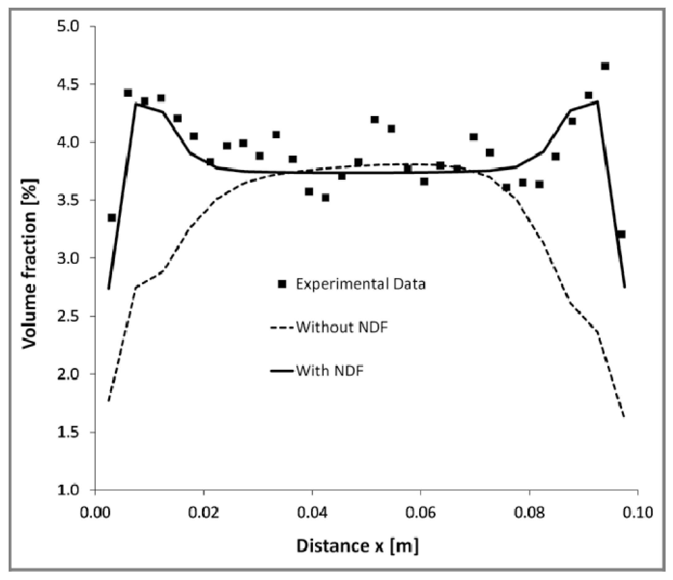
[45][74]Without NDF:
(B) 26.65
With NDF:
(A) 10.38
(B) 9.46
Without NDF
Evaluated at U G = 0.15 cm/s:
(B) 18.79
Evaluated at U G = 0.5 cm/s:
(B) 15.56
Evaluated at U G = 1 cm/s:
(B) 19.01
With NDF
Evaluated at U G = 0.15 cm/s:
(A) 22.02
(B) 20.89
Evaluated at U G = 0.5 cm/s:
(A) 21.68
(B) 14.03
Evaluated at U G = 1 cm/s:
(A) 21.7
(B) 17.60
Without NDF
Evaluated at U G = 0.15 cm/s:
(B) 32.67
Evaluated at U G = 0.5 cm/s:
(B) 32.41
Evaluated at U G = 1 cm/s:
(B) 30.48
With NDF
Evaluated at U G = 0.15 cm/s:
(A) 33.02
(B) 13.74
Evaluated at U G = 0.5 cm/s:
(A) 20.80
(B) 36.39
Evaluated at U G = 1 cm/s:
(A) 15.30
(B) 27.31
[71][96]-Evaluated at U G = 0.3 cm/s:
(1A α ) 4.19
(1A β ) 12.22
(1B α ) 4.19
(1C α ) 4.19
(1D α ) 4.19
(1E α ) 9.43
(1F α ) 6.98
Evaluated at U G = 1.3 cm/s:
(1A α ) 14.42
(2A α ) 6.48
(2A β ) 20.34
(2B α ) 8.95
(2C α ) 6.73
(2D α ) 7.49
(2E α ) 8.31
(2F α ) 7.85
(2G α ) 9.36
Evaluated at U G = 0.3 cm/s:
(1A α ) 44.27
(1A β ) 44.27
(1B α ) 44.45
(1C α ) 44.45
(1D α ) 48.18
(1E α ) 43.27
(1F α ) 40.32
Evaluated at U G = 1.3 cm/s:
(1A α ) 47.48
(2A α ) 30.20
(2A β ) 39.28
(2B α ) 41.57
(2C α ) 57.50
(2D α ) 41.67
(2E α ) 47.58
(2F α ) 45.75
(2G α ) 80.64
[80][56]-(1A β ) 21
(2B α ) 9.96
(2B β ) 21.44
(2C α ) 9.68
(2C β ) 21.53
(1A β ) 21.25
(2B α ) 29.89
(2B β ) 32.31
(2C α ) 22.26
(2C β ) 37.05
[81][97]-Evaluated at U G = 8 cm/s:
(1A α ) 15.37
(1B α ) 23.31
(2A α ) 20.46
(2B α ) 22.29
Evaluated at U G = 12 cm/s:
(1A α ) 20.80
(1A β ) 75.80
-
[82][98](A) 14.76
(B) 9.45
(C) 6.18
(D) 22.75
--
[83][99]-(1A α ) 8.66
(2A α ) 10.96
(1A β ) 9.60
(2A β ) 27.70
(1B α ) 5.17
(1B β ) 11.67
[88][96]-(A) 9.44
(B) 8.88
(C) 8.65
(A) 31.31
(B) 63.34
(C) 53.57
[89][89](1C) 42.01
(2C) 39.55
(2A) 35.87
(2B) 7.99
Evaluated at U G = 16 cm/s:
(2B) 6.67
-
[84][100](1A) 3.32
(1B) 12.63
(1C) 15.02
(1F) 32.53
(2F) 3.87
Evaluated at U G = 1.9 cm/s:
(1A) 10.85
(1B) 13.39
(1C) 13.3
(1D) 15.93
(1E) 20.57
(1F) 23.15
(2C) 3.65
(2D) 3.69
(2E) 4.11
(2F) 6.82
Evaluated at U G = 3.8 cm/s:
(1A) 16.6
(1B) 29.54
(1C) 34.91
(1F) 50
(2F) 9.9
-
[90][101](1A) 6.69
(2B) 7.78
Evaluated at U G = 16 cm/s:
(1B) 12.48
(2B) 8.94
Evaluated at U G = 16 cm/s:
(1B) 35.25
(2B) 33.78
[91][91]13.67--
[30][89](A) 84.77
(B) 44.40
(C) 54.91
(D) 29.82
(E) 2.83
Evaluated at U G = 3 cm/s:
(E) 5.70
Evaluated at U G = 16 cm/s:
(E) 4.07
Evaluated at U G = 3 cm/s:
(E) 38.39
Evaluated at U G = 16 cm/s:
(E) 25.18
[20][102]-8.07
No lift:
42.99
No turbulent dispersion:
23.86
No wall lubrication:
12.64
No virtual mass:
8.99
No BIT:
9.32
-

5. Conclusions

This paper has presented a detailed review of CFD modelling of two-phase bubble columns. The models most commonly adopted for interfacial momentum exchange, bubble-induced turbulence, coalescence, and breakup are described. A quantitative comparison between the different modelling approaches is presented in Section 4, considering various studies from the literature and computing the relative errors between the CFD predictions and the experimental data.
On the basis of the literature review presented in this work, the following recommendations are made for future studies:
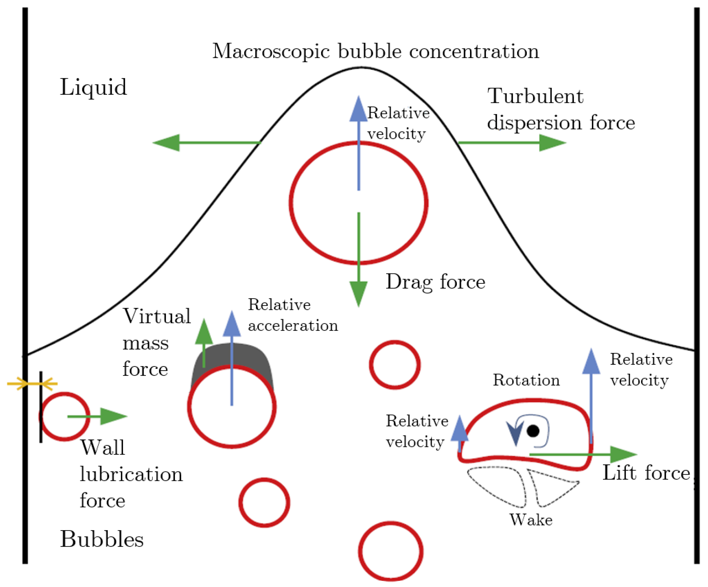
  • Concerning the interfacial forces, the momentum transfer between the phases is dominated by the drag force. For a proper description of the drag coefficient, the models of Tomiyama et al. (1998) [19], Grace et al. (1976) [16], and Ishii and Zuber (1978) [17] can be implemented; however, they should be corrected with a swarm factor. When presenting numerical studies, a sensitivity analysis among the different models should be performed.
    The lift, wall lubrication, and turbulence dispersion forces should be added to the model to obtain more accurate solutions. In particular, a correlation that predicts the change in the sign of the lift coefficient should be considered.
  • Concerning the turbulence modelling, RANS models, in particular the k ε RNG and the k ω SST models, provide satisfying results in terms of average quantities. The LES turbulence model provides better results in the near-sparger region, where the flow is more anisotropic. However, no remarkable differences compared to the RANS methods have been highlighted in the fully developed region.
  • The modelling approach of the dispersed phase (i.e., mono-dispersed, MUSIG, iMUSIG, PBM) should always be related to the simulated flow regime. A mono-dispersed approximation applies at very low superficial gas velocities. Conversely, multiple-size models that include coalescence and breakup should be considered.
  • Regarding the numerical settings, high-order resolution discretization schemes should be used in order to prevent or reduce numerical discretization errors as much as possible.
Finally, it can be concluded that detailed comprehension of the phenomena governing multiphase flows remains needed, and additional effort should be spend on developing a fully predictive a priori CFD model.

Author Contributions

N.V. conducted the literature survey, post-processed the literature data, and wrote the paper. G.B. and R.M. were responsible for conceptualization, methodology, and revision. All authors have read and agreed to the published version of the manuscript.

Funding

This research received no external funding.

Data Availability Statement

The data presented in this study are available on request from the corresponding author.

Conflicts of Interest

The authors declare no conflict of interest.

Nomenclature

BITBubble-Induced Turbulence
CFDComputational Fluid Dynamics
CMClass Method
DNSDirect Numerical Simulation
LDALaser Doppler Velocimetry
LESLarge Eddy Simulation
NDFNumber Density Function
PBMPopulation Balance Model
PBEPopulation Balance Equation
PIVParticle Image Velocimetry
PSVParticle Shadowgraph Velocimetry
QMOMQuadrature Method of Moment
RANSReynolds-Averaged NavierStokes
RSMReynolds Stress Models
u Local velocity[m/s]
C D Drag coefficient[-]
C L Lift coefficient[-]
C T D Turbulent dispersion coefficient                                                           [-]
C W L Wall lubrication coefficient[-]
C V M Virtual mass coefficient[-]
d b Bubble diameter[m]
d e q Equivalent bubble diameter[m]
D H * Non-dimensional diameter[-]
D c r * Critical non-dimensional diameter[-]
D H Hydraulic diameter[m]
EBubble aspect ratio[-]
E o Eötvös number[m]
F D Drag force[kg/ m 2 s 2 ]
F L Lift force[kg/ m 2 s 2 ]
F T D Turbulent dispersion force[kg/ m 2 s 2 ]
F W L Wall lubrication force[kg/ m 2 s 2 ]
F V M Virtual mass force[kg/ m 2 s 2 ]
gAcceleration due to gravity[m/ s 2 ]
g ( V b ) Breakup frequency[ 1 / s ]
hSwarm factor[-]
h ( d b , i , d b , j ) Collision frequency[ 1 / s ]
J T Drift flux[m/s]
kTurbulent kinetic energy[ m 2 / s 2 ]
M I Momentum exchanges[kg/ m 2 s 2 ]
M o Morton number[-]
pPressure[Pa]
R e b Bubble Reynolds number
STotal source/sink term in the population balance equation[ m 2 /s]
S b Total source/sink term due to breakup[ m 3 /s]
S c Total source/sink term due to coalescence[ m 3 /s]
S m Total source/sink term due to mass transfer[ m 3 /s]
S p Total source/sink term due to pressure change[ m 3 /s]
S p h Total source/sink term due to phase change[ m 3 /s]
S r Total source/sink term due to reaction[ m 3 /s]
U G Superficial gas velocity[m/s]
U L Superficial liquid velocity[m/s]
V b Bubble volume in population balance equation[ m 3 ]
α G Local gas volume fraction[-]
β Daughter distribution function[-]
ε G Global gas holdup[-]
ε Turbulent dissipation rate[ m 2 / s 3 ]
λ ( d b , i , d b , j ) Coalescence efficiency[-]
μ Dynamic viscosity[ kg / m / s ]
μ t Turbulent viscosity[ m 2 / s ]
ω Specific dissipation rate[ 1 / s ]
ρ Density[ kg / m 3 ]
σ Surface tension[kg/ m 2 s 2
τ ¯ Viscous stress tensor[ kg / m / s 2 ]
GGas phase
LLiquid phase
kk-th phase

References

  1. Kantarci, N.; Borak, F.; Ulgen, K.O. Bubble column reactors. Process Biochem. 2005, 40, 2263–2283. [Google Scholar] [CrossRef]
  2. Buffo, A.; Marchisio, D.L. Modeling and simulation of turbulent polydisperse gas-liquid systems via the generalized population balance equation. Rev. Chem. Eng. 2014, 30, 73–126. [Google Scholar] [CrossRef]
  3. Khan, K.I. Fluid Dynamic Modeling of Bubble Column Reactor. Ph.D Thesis, Politecnico di Torino, Torino, Italy, 2014. [Google Scholar]
  4. Wu, B.; Firouzi, M.; Mitchell, T.; Rufford, T.E.; Leonardi, C.; Towler, B. A critical review of flow maps for gas-liquid flows in vertical pipes and annuli. Chem. Eng. J. 2017, 326, 350–377. [Google Scholar] [CrossRef] [Green Version]
  5. Kitscha, J.; Kocamustafaogullari, G. Breakup criteria for fluid particles. Int. J. Multiph. Flow 1989, 15, 573–588. [Google Scholar] [CrossRef]
  6. Brooks, C.S.; Paranjape, S.S.; Ozar, B.; Hibiki, T.; Ishii, M. Two-group drift-flux model for closure of the modified two-fluid model. Int. J. Heat Fluid Flow 2012, 37, 196–208. [Google Scholar] [CrossRef]
  7. Besagni, G. Bubble column fluid dynamics: A novel perspective for flow regimes and comprehensive experimental investigations. Int. J. Multiph. Flow 2021, 135, 103510. [Google Scholar] [CrossRef]
  8. Krepper, E.; Lucas, D.; Prasser, H.M. On the modelling of bubbly flow in vertical pipes. Nucl. Eng. Des. 2005, 235, 597–611. [Google Scholar] [CrossRef]
  9. Lapin, A.; Lübbert, A. Numerical simulation of the dynamics of two-phase gas–liquid flows in bubble columns. Chem. Eng. Sci. 1994, 49, 3661–3674. [Google Scholar] [CrossRef]
  10. Buwa, V.V.; Deo, D.S.; Ranade, V.V. Eulerian–Lagrangian simulations of unsteady gas–liquid flows in bubble columns. Int. J. Multiph. Flow 2006, 32, 864–885. [Google Scholar] [CrossRef]
  11. Besbes, S.; El Hajem, M.; Aissia, H.B.; Champagne, J.; Jay, J. PIV measurements and Eulerian–Lagrangian simulations of the unsteady gas–liquid flow in a needle sparger rectangular bubble column. Chem. Eng. Sci. 2015, 126, 560–572. [Google Scholar] [CrossRef]
  12. Khan, I.; Wang, M.; Zhang, Y.; Tian, W.; Su, G.; Qiu, S. Two-phase bubbly flow simulation using CFD method: A review of models for interfacial forces. Prog. Nucl. Energy 2020, 125, 103360. [Google Scholar] [CrossRef]
  13. Suh, J.W.; Kim, J.W.; Choi, Y.S.; Kim, J.H.; Joo, W.G.; Lee, K.Y. Development of numerical Eulerian-Eulerian models for simulating multiphase pumps. J. Pet. Sci. Eng. 2018, 162, 588–601. [Google Scholar] [CrossRef]
  14. Schiller, L. A drag coefficient correlation. Zeit. Ver. Deutsch. Ing. 1933, 77, 318–320. [Google Scholar]
  15. Frank. Viscous Fluid Flow; McGraw-Hill: New York, NY, USA, 1974. [Google Scholar]
  16. Grace, J.R. Shapes and velocities of single drops and bubbles moving freely through immiscible liquids. Trans. Inst. Chem. Eng. 1976, 54, 167. [Google Scholar]
  17. Ishii, M.; Zuber, N. Drag coefficient and relative velocity in bubbly, droplet or particulate flows. AIChE J. 1979, 25, 843–855. [Google Scholar] [CrossRef]
  18. Grevskott, S.; Sannaes, B.; Duduković, M.; Hjarbo, K.; Svendsen, H. Liquid circulation, bubble size distributions, and solids movement in two-and three-phase bubble columns. Chem. Eng. Sci. 1996, 51, 1703–1713. [Google Scholar] [CrossRef]
  19. Tomiyama, A. Struggle with computational bubble dynamics. Multiph. Sci. Technol. 1998, 10, 369–405. [Google Scholar]
  20. Zhang, D.; Deen, N.; Kuipers, J. Numerical simulation of the dynamic flow behavior in a bubble column: A study of closures for turbulence and interface forces. Chem. Eng. Sci. 2006, 61, 7593–7608. [Google Scholar] [CrossRef]
  21. Dijkhuizen, W.; Roghair, I.; Annaland, M.V.S.; Kuipers, J. DNS of gas bubbles behaviour using an improved 3D front tracking model—Drag force on isolated bubbles and comparison with experiments. Chem. Eng. Sci. 2010, 65, 1415–1426. [Google Scholar] [CrossRef]
  22. Bridge, A.; Lapidus, L.; Elgin, J. The mechanics of vertical gas-liquid fluidized system I: Countercurrent flow. AIChE J. 1964, 10, 819–826. [Google Scholar] [CrossRef]
  23. Wallis, G.B. One-Dimensional Two-Phase Flow; McGraw-Hill: New York, NY, USA, 1969. [Google Scholar]
  24. Rusche, H.; Issa, R. The effect of voidage on the drag force on particles, droplets and bubbles in dispersed two-phase flow. In Proceedings of the Japanese European Two-Phase Flow Meeting, Tshkuba, Japan, 25–29 September 2000. [Google Scholar]
  25. Roghair, I.; Lau, Y.; Deen, N.; Slagter, H.; Baltussen, M.; Annaland, M.V.S.; Kuipers, J. On the drag force of bubbles in bubble swarms at intermediate and high Reynolds numbers. Chem. Eng. Sci. 2011, 66, 3204–3211. [Google Scholar] [CrossRef]
  26. Buffo, A.; Vanni, M.; Renze, P.; Marchisio, D.L. Empirical drag closure for polydisperse gas–liquid systems in bubbly flow regime: Bubble swarm and micro-scale turbulence. Chem. Eng. Res. Des. 2016, 113, 284–303. [Google Scholar] [CrossRef]
  27. Simonnet, M.; Gentric, C.; Olmos, E.; Midoux, N. CFD simulation of the flow field in a bubble column reactor: Importance of the drag force formulation to describe regime transitions. Chem. Eng. Process. Process Intensif. 2008, 47, 1726–1737. [Google Scholar] [CrossRef]
  28. McClure, D.D.; Norris, H.; Kavanagh, J.M.; Fletcher, D.F.; Barton, G.W. Validation of a computationally efficient computational fluid dynamics (CFD) model for industrial bubble column bioreactors. Ind. Eng. Chem. Res. 2014, 53, 14526–14543. [Google Scholar] [CrossRef]
  29. McClure, D.D.; Kavanagh, J.M.; Fletcher, D.F.; Barton, G.W. Experimental investigation into the drag volume fraction correction term for gas-liquid bubbly flows. Chem. Eng. Sci. 2017, 170, 91–97. [Google Scholar] [CrossRef]
  30. Gemello, L.; Cappello, V.; Augier, F.; Marchisio, D.; Plais, C. CFD-based scale-up of hydrodynamics and mixing in bubble columns. Chem. Eng. Res. Des. 2018, 136, 846–858. [Google Scholar] [CrossRef]
  31. Yang, G.; Zhang, H.; Luo, J.; Wang, T. Drag force of bubble swarms and numerical simulations of a bubble column with a CFD-PBM coupled model. Chem. Eng. Sci. 2018, 192, 714–724. [Google Scholar] [CrossRef]
  32. Tomiyama, A.; Tamai, H.; Zun, I.; Hosokawa, S. Transverse migration of single bubbles in simple shear flows. Chem. Eng. Sci. 2002, 57, 1849–1858. [Google Scholar] [CrossRef]
  33. Wellek, R.; Agrawal, A.; Skelland, A. Shape of liquid drops moving in liquid media. AIChE J. 1966, 12, 854–862. [Google Scholar] [CrossRef]
  34. Ziegenhein, T.; Lucas, D. The critical bubble diameter of the lift force in technical and environmental, buoyancy-driven bubbly flows. Int. J. Multiph. Flow 2019, 116, 26–38. [Google Scholar] [CrossRef]
  35. Besagni, G.; Inzoli, F.; De Guido, G.; Pellegrini, L.A. Experimental investigation on the influence of ethanol on bubble column hydrodynamics. Chem. Eng. Res. Des. 2016, 112, 1–15. [Google Scholar] [CrossRef]
  36. Ziegenhein, T.; Tomiyama, A.; Lucas, D. A new measuring concept to determine the lift force for distorted bubbles in low Morton number system: Results for air/water. Int. J. Multiph. Flow 2018, 108, 11–24. [Google Scholar] [CrossRef]
  37. Behzadi, A.; Issa, R.; Rusche, H. Modelling of dispersed bubble and droplet flow at high phase fractions. Chem. Eng. Sci. 2004, 59, 759–770. [Google Scholar] [CrossRef]
  38. Simonin, O.; Viollet, P. Modelling of turbulent two-phase jets loaded with discrete particles. In Phenomena in Multiphase Flows; Hemisphere Publishing Corporation: London, UK, 1990; Volume 1990, pp. 259–269. [Google Scholar]
  39. Burns, A.D.; Frank, T.; Hamill, I.; Shi, J.M. The Favre averaged drag model for turbulent dispersion in Eulerian multi-phase flows. In Proceedings of the 5th International Conference on Multiphase Flow, ICMF, Yokohama, Japan, 30 May–4 June 2004; Volume 4, pp. 1–17. [Google Scholar]
  40. Lopez de Bertodano, M.; Moraga, F.; Drew, D.; Lahey, R., Jr. The modeling of lift and dispersion forces in two-fluid model simulations of a bubbly jet. J. Fluids Eng. 2004, 126, 573–577. [Google Scholar] [CrossRef]
  41. Antal, S.; Lahey, R., Jr.; Flaherty, J. Analysis of phase distribution in fully developed laminar bubbly two-phase flow. Int. J. Multiph. Flow 1991, 17, 635–652. [Google Scholar] [CrossRef]
  42. Tomiyama, A. Effects of Eotvos number and dimensionless liquid volumetric flux on lateral motion of a bubble in a laminar duct flow. In Proceedings of the 2nd International Conference on Multiphase Flow, Kyoto, Japan, 3–7 April 1995; Volume 3. [Google Scholar]
  43. Hosokawa, S.; Tomiyama, A.; Misaki, S.; Hamada, T. Lateral migration of single bubbles due to the presence of wall. In Proceedings of the Fluids Engineering Division Summer Meeting, Montreal, QC, Canada, 14–18 July 2002; Volume 36150, pp. 855–860. [Google Scholar]
  44. Frank, T. Advances in computational fluid dynamics (CFD) of 3-dimensional gas-liquid multiphase flows. In Proceedings of the NAFEMS Seminar: Simulation of Complex Flows (CFD)–Applications and Trends, Wiesbaden, Germany, 25–26 April 2005; pp. 1–18. [Google Scholar]
  45. Ziegenhein, T.; Rzehak, R.; Krepper, E.; Lucas, D. Numerical simulation of polydispersed flow in bubble columns with the inhomogeneous multi-size-group model. Chem. Ing. Tech. 2013, 85, 1080–1091. [Google Scholar] [CrossRef]
  46. Tabib, M.V.; Roy, S.A.; Joshi, J.B. CFD simulation of bubble column—An analysis of interphase forces and turbulence models. Chem. Eng. J. 2008, 139, 589–614. [Google Scholar] [CrossRef]
  47. Yeoh, G.; Tu, J. Basic theory and conceptual framework of multiphase flows. In Handbook of Multiphase Flow Science and Technology; Springer: Berlin, Germany, 2017; pp. 1–47. [Google Scholar]
  48. Liao, Y.; Lucas, D. A literature review on mechanisms and models for the coalescence process of fluid particles. Chem. Eng. Sci. 2010, 65, 2851–2864. [Google Scholar] [CrossRef]
  49. Liao, Y.; Lucas, D. A literature review of theoretical models for drop and bubble breakup in turbulent dispersions. Chem. Eng. Sci. 2009, 64, 3389–3406. [Google Scholar] [CrossRef]
  50. Prince, M.J.; Blanch, H.W. Bubble coalescence and break-up in air-sparged bubble columns. AIChE J. 1990, 36, 1485–1499. [Google Scholar] [CrossRef]
  51. Luo, H.; Svendsen, H.F. Theoretical model for drop and bubble breakup in turbulent dispersions. AIChE J. 1996, 42, 1225–1233. [Google Scholar] [CrossRef]
  52. Martínez-Bazán, C.; Montañés, J.L.; Lasheras, J.C. On the breakup of an air bubble injected into a fully developed 881 turbulent flow. Part 1. Breakup frequency. J. Fluid Mech. 1999, 401, 157–182. [Google Scholar] [CrossRef] [Green Version]
  53. Martínez-Bazán, C.; Montañés, J.L.; Lasheras, J.C. On the breakup of an air bubble injected into a fully developed 883 turbulent flow. Part 2. Size PDF of the resulting daughter bubbles. J. Fluid Mech. 1999, 401, 183–207. [Google Scholar] [CrossRef] [Green Version]
  54. Batchelor, G.K. The Theory of Homogeneous Turbulence; Cambridge University Press: Cambridge, UK, 1953. [Google Scholar]
  55. Lehr, F.; Millies, M.; Mewes, D. Bubble-size distributions and flow fields in bubble columns. AIChE J. 2002, 48, 2426–2443. [Google Scholar] [CrossRef]
  56. Chen, J.; Li, F.; Degaleesan, S.; Gupta, P.; Al-Dahhan, M.H.; Dudukovic, M.P.; Toseland, B.A. Fluid dynamic parameters in bubble columns with internals. Chem. Eng. Sci. 1999, 54, 2187–2197. [Google Scholar] [CrossRef]
  57. Shinnar, R.; Church, J.M. Statistical theories of turbulence in predicting particle size in agitated dispersions. Ind. Eng. Chem. 1960, 52, 253–256. [Google Scholar] [CrossRef]
  58. Howarth, W. Coalescence of drops in a turbulent flow field. Chem. Eng. Sci. 1964, 19, 33–38. [Google Scholar] [CrossRef]
  59. Coulaloglou, C.; Tavlarides, L.L. Description of interaction processes in agitated liquid-liquid dispersions. Chem. Eng. Sci. 1977, 32, 1289–1297. [Google Scholar] [CrossRef]
  60. Chesters, A. Modelling of coalescence processes in fluid-liquid dispersions: A review of current understanding. Chem. Eng. Res. Des. 1991, 69, 259–270. [Google Scholar]
  61. Luo, H. Coalescence, Breakup and Liquid Circulation in Bubble Column Reactors. Ph.D. Thesis, Department of Chemical Engineering, The University of Trondheim, Trondheim, Norvey, 1993. [Google Scholar]
  62. Sanyal, J.; Marchisio, D.L.; Fox, R.O.; Dhanasekharan, K. On the comparison between population balance models for CFD simulation of bubble columns. Ind. Eng. Chem. Res. 2005, 44, 5063–5072. [Google Scholar] [CrossRef] [Green Version]
  63. McGraw, R. Description of aerosol dynamics by the quadrature method of moments. Aerosol Sci. Technol. 1997, 27, 255–265. [Google Scholar] [CrossRef]
  64. Marchisio, D.L.; Vigil, R.D.; Fox, R.O. Quadrature method of moments for aggregation–breakage processes. J. Colloid Interface Sci. 2003, 258, 322–334. [Google Scholar] [CrossRef]
  65. Petitti, M.; Vanni, M.; Marchisio, D.L.; Buffo, A.; Podenzani, F. Simulation of coalescence, break-up and mass transfer in a gas–liquid stirred tank with CQMOM. Chem. Eng. J. 2013, 228, 1182–1194. [Google Scholar] [CrossRef]
  66. Ma, T.; Lucas, D.; Ziegenhein, T.; Fröhlich, J.; Deen, N. Scale-Adaptive Simulation of a square cross-sectional bubble column. Chem. Eng. Sci. 2015, 131, 101–108. [Google Scholar] [CrossRef]
  67. Dhotre, M.; Deen, N.; Niceno, B.; Khan, Z.; Joshi, J. Large eddy simulation for dispersed bubbly flows: A review. Int. J. Chem. Eng. 2013, 2013, 343276. [Google Scholar] [CrossRef]
  68. Masood, R.; Rauh, C.; Delgado, A. CFD simulation of bubble column flows: An explicit algebraic Reynolds stress model approach. Int. J. Multiph. Flow 2014, 66, 11–25. [Google Scholar] [CrossRef]
  69. Parekh, J.; Rzehak, R. Euler–Euler multiphase CFD-simulation with full Reynolds stress model and anisotropic bubble-induced turbulence. Int. J. Multiph. Flow 2018, 99, 231–245. [Google Scholar] [CrossRef]
  70. Joshi, J. Computational flow modelling and design of bubble column reactors. Chem. Eng. Sci. 2001, 56, 5893–5933. [Google Scholar] [CrossRef]
  71. Ziegenhein, T.; Lucas, D.; Rzehak, R.; Krepper, E. Closure relations for CFD simulation of bubble columns. In Proceedings of the 8th International Conference on Multiphase Flow—ICMF 2014, Jeju, Republic of Korea, 26–31 May 2013. [Google Scholar]
  72. Morel, C. Turbulence modelling and first numerical simulations in turbulent two-phase flows. In Proceedings of the 11th Symposium on Turbulent Shear Flows, Grenoble, France, 8–11 September 1997; Volume 3. [Google Scholar]
  73. Troshko, A.; Hassan, Y. A two-equation turbulence model of turbulent bubbly flows. Int. J. Multiph. Flow 2001, 27, 1965–2000. [Google Scholar] [CrossRef]
  74. Pfleger, D.; Becker, S. Modelling and simulation of the dynamic flow behaviour in a bubble column. Chem. Eng. Sci. 2001, 56, 1737–1747. [Google Scholar] [CrossRef]
  75. Politano, M.; Carrica, P.; Converti, J. A model for turbulent polydisperse two-phase flow in vertical channels. Int. J. Multiph. Flow 2003, 29, 1153–1182. [Google Scholar] [CrossRef]
  76. Rzehak, R.; Krepper, E. Bubble-induced turbulence: Comparison of CFD models. Nucl. Eng. Des. 2013, 258, 57–65. [Google Scholar] [CrossRef]
  77. Sato, Y.; Sekoguchi, K. Liquid velocity distribution in two-phase bubble flow. Int. J. Multiph. Flow 1975, 2, 79–95. [Google Scholar] [CrossRef]
  78. Chen, P.; Sanyal, J.; Duduković, M. Numerical simulation of bubble columns flows: Effect of different breakup and coalescence closures. Chem. Eng. Sci. 2005, 60, 1085–1101. [Google Scholar] [CrossRef]
  79. Ekambara, K.; Dhotre, M. CFD simulation of bubble column. Nucl. Eng. Des. 2010, 240, 963–969. [Google Scholar] [CrossRef]
  80. Xu, L.; Yuan, B.; Ni, H.; Chen, C. Numerical simulation of bubble column flows in churn-turbulent regime: Comparison of bubble size models. Ind. Eng. Chem. Res. 2013, 52, 6794–6802. [Google Scholar] [CrossRef]
  81. McClure, D.D.; Kavanagh, J.M.; Fletcher, D.F.; Barton, G.W. Development of a CFD model of bubble column bioreactors: Part two—Comparison of experimental data and CFD predictions. Chem. Eng. Technol. 2014, 37, 131–140. [Google Scholar] [CrossRef]
  82. Masood, R.; Delgado, A. Numerical investigation of the interphase forces and turbulence closure in 3D square bubble columns. Chem. Eng. Sci. 2014, 108, 154–168. [Google Scholar] [CrossRef]
  83. Liu, Y.; Hinrichsen, O. Study on CFD–PBM turbulence closures based on k–ε and Reynolds stress models for heterogeneous bubble column flows. Comput. Fluids 2014, 105, 91–100. [Google Scholar] [CrossRef]
  84. Syed, A.H.; Boulet, M.; Melchiori, T.; Lavoie, J.M. CFD simulations of an air-water bubble column: Effect of Luo coalescence parameter and breakup kernels. Front. Chem. 2017, 5, 68. [Google Scholar] [CrossRef]
  85. Zhang, X.B.; Yan, W.C.; Luo, Z.H. CFD-PBM Simulation of Bubble Columns: Sensitivity Analysis of the Nondrag Forces. Ind. Eng. Chem. Res. 2020, 59, 18674–18682. [Google Scholar] [CrossRef]
  86. Deen, N.G.; Hjertager, B.H.; Solberg, T. Comparison of PIV and LDA measurement methods applied to the gas-liquid flow in a bubble column. In Proceedings of the 10th International Symposium on Applications of Laser Techniques to Fluid Mechanics, Lisbon, Portugal, 10–13 July 2000; pp. 1–12. [Google Scholar]
  87. Ziegenhein, T.; Lucas, D.; Besagni, G.; Inzoli, F. Experimental study of the liquid velocity and turbulence in a large-scale air-water counter-current bubble column. Exp. Therm. Fluid Sci. 2020, 111, 109955. [Google Scholar] [CrossRef]
  88. Ziegenhein, T.; Rzehak, R.; Lucas, D. Transient simulation for large scale flow in bubble columns. Chem. Eng. Sci. 2015, 122, 1–13. [Google Scholar] [CrossRef]
  89. Raimundo, P.M. Analysis and Modelization of Local Hydrodynamics in Bubble Columns. Ph.D. Thesis, Université Grenoble Alpes, Grenoble, France, 2015. [Google Scholar]
  90. Fletcher, D.F.; McClure, D.D.; Kavanagh, J.M.; Barton, G.W. CFD simulation of industrial bubble columns: Numerical challenges and model validation successes. Appl. Math. Model. 2017, 44, 25–42. [Google Scholar] [CrossRef]
  91. Saleh, S.N.; Mohammed, A.A.; Al-Jubory, F.K.; Barghi, S. CFD assesment of uniform bubbly flow in a bubble column. J. Pet. Sci. Eng. 2018, 161, 96–107. [Google Scholar] [CrossRef]
  92. Liang, X.F.; Pan, H.; Su, Y.H.; Luo, Z.H. CFD-PBM approach with modified drag model for the gas–liquid flow in a bubble column. Chem. Eng. Res. Des. 2016, 112, 88–102. [Google Scholar] [CrossRef]
  93. Degaleesan, S. Fluid Dynamic Measurements and Modeling of Liquid Mixing in Bubble Columns; Washington University in St. Louis: St. Louis, MO, USA, 1997. [Google Scholar]
  94. Menzel, T.; In der Weide, T.; Staudacher, O.; Wein, O.; Onken, U. Reynolds shear stress for modeling of bubble column reactors. Ind. Eng. Chem. Res. 1990, 29, 988–994. [Google Scholar] [CrossRef]
  95. Kulkarni, A.; Ekambara, K.; Joshi, J. On the development of flow pattern in a bubble column reactor: Experiments and CFD. Chem. Eng. Sci. 2007, 62, 1049–1072. [Google Scholar] [CrossRef]
  96. bin Mohd Akbar, M.H.; Hayashi, K.; Hosokawa, S.; Tomiyama, A. Bubble tracking simulation of bubble-induced pseudoturbulence. Multiph. Sci. Technol. 2012, 24, 197–222. [Google Scholar] [CrossRef]
  97. McClure, D.D.; Kavanagh, J.M.; Fletcher, D.F.; Barton, G.W. Development of a CFD model of bubble column bioreactors: Part one—A detailed experimental study. Chem. Eng. Technol. 2013, 36, 2065–2070. [Google Scholar] [CrossRef]
  98. Deen, N. An Experimental and Computational Study of Fluid Dynamics in Gas-Liquid Chemical Reactors; Aalborg University Esbjerg: Esbjerg, Denmark, 2001. [Google Scholar]
  99. Rampure, M.R.; Kulkarni, A.A.; Ranade, V.V. Hydrodynamics of bubble column reactors at high gas velocity: Experiments and computational fluid dynamics (CFD) simulations. Ind. Eng. Chem. Res. 2007, 46, 8431–8447. [Google Scholar] [CrossRef]
  100. Hills, J.H. Radial non-uniformity of velocity and voidage in a bubble column. Trans. Inst. Chem. Eng. 1974, 52, 1–9. [Google Scholar]
  101. McClure, D.D.; Wang, C.; Kavanagh, J.M.; Fletcher, D.F.; Barton, G.W. Experimental investigation into the impact of sparger design on bubble columns at high superficial velocities. Chem. Eng. Res. Des. 2016, 106, 205–213. [Google Scholar] [CrossRef]
  102. Guan, X.; Yang, N. Bubble properties measurement in bubble columns: From homogeneous to heterogeneous regime. Chem. Eng. Res. Des. 2017, 127, 103–112. [Google Scholar] [CrossRef]
Figure 1. Bubble column reactor.
Fluids 08 00091 g001
Figure 2. Representation of flow regimes in vertical pipes. Reprinted with permission from [4].
Fluids 08 00091 g002
Figure 3. Flow regimes and regime transitions in a large-diameter bubble column. Reprinted with permission from [7].
Fluids 08 00091 g003
Figure 4. Flow pattern evolution in two-phase bubble columns. Reprinted with permission from [8].
Fluids 08 00091 g004
Figure 6. Evolution of the drag coefficient with respect to the bubble diameter at | u G u L | = 0.1 m/s for air bubbles in water. Comparison between the correlations of Schiller and Naumann (1933) [14], Grace et al. (1976) [16], Ishii and Zuber (1978) [17], Grevskott et al. (1996) [18] and Tomiyama (1998) [19].
Fluids 08 00091 g006
Figure 7. Comparison of published Swarm factor as a function of local void fraction for bubbles with d b of 6.5 mm. Comparison between the correlations of Bridge et al. (1964) [22], Wallis (1969) [23], Ishii and Zuber (1979) [17], Rusche and Issa (2000) [24], Simonnet et al. (2008) [27], Roghair et al. (2011) [25] and Buffo et al. (2016) [26]. Note the discrepancy between the correlation proposed by Simonnet et al. (2008) [27] and the others.
Fluids 08 00091 g007
Figure 8. Drag correction factors that reduce the drag force in bubble swarms for bubbles with d b of 6.5 mm. Comparison between the correlations of McClure et al. (2014c) [28], McClure et al. (2017) [29], Gemello et al. (2018) [30] and Yang et al. [31].
Fluids 08 00091 g008
Figure 9. Comparison between Tomiyama et al. (2002b) [32] and Ziegenhein et al. (2018) [34] models for the lift coefficient.
Fluids 08 00091 g009
Figure 10. Influence of Non-Drag-Forces (NDF), (with the exception of the virtual mass force) on the local void fraction profile. Reprinted with permission from [45].
Fluids 08 00091 g010
Figure 11. Breakup mechanisms.
Fluids 08 00091 g011
Figure 12. Coalescence mechanisms.
Fluids 08 00091 g012
Table 2. Applicable breakup models for simulated bubble column.
AuthorBreakage Frequency (g)Daughter Size Distribution ( β )
Prince and Blanch (1990) [50] g = 0.2 d b , j d b , j 0.07 π 4 λ ε d b , j + λ ε 2 d b , j 2 / 3 + λ ε 2 / 3 0.5 ε 1 / 3 × exp 1.18 λ ε 2 / 3 σ ρ L d b , j ε 2 / 3 d λ ε Uniform
Luo and Svendsen (1996) [51] g = 1 2 0 1 0.923 1 α G n ε d b , j 2 1 / 3 × ξ min 1 ( 1 + ξ ) 2 ξ 11 / 13 exp 12 c f σ c β ρ L ε 2 / 3 d b , j 5 / 3 ξ 11 / 13 d ξ d f b v with ξ = λ ε d b , c f = f b v 2 / 3 + 1 f b v 2 / 3 1 , f b v = d b , i 3 d b , i 3 + d b , j 3 , c β = 2 β = 2 ξ min 1 ( 1 + ξ ) 2 ξ 11 / 3 exp χ c d ξ V i 0 1 ξ min 1 ( 1 + ξ ) 2 ξ 11 / 3 exp χ c d ξ d f b v with χ c = 12 c f σ c β ρ 1 ε 2 / 3 d b , i 5 / 3 ξ 11 / 3
Martïnez and Bazän (1999) [52,53] g = K g n β ε d b , j 2 / 3 12 σ / ρ c d b , j d b , j with β = 8.2 [54], K g = 0.25 β = D * 2 / 3 Λ 5 / 3 1 D * 3 2 / 9 Λ 5 / 3 D min * D max D * 2 / 3 Λ 5 / 3 1 D * 3 2 / 9 Λ 5 / 3 d D * with D * = d b , j d b , i , Λ = ( 12 σ β ρ L ) , β = 8.2 [54]
Lehr et al. (2002) [55] g = 0.5 d b , j 5 / 3 ε 19 / 15 ρ L 7 / 5 σ 7 / 5 exp 2 σ 9 / 5 ρ L d b , j 9 / 5 ε 6 / 5 L 3 β = 1 π f b v exp 9 4 ln 2 2 / 5 d b , j ρ L 3 / 5 ε 2 / 5 σ 3 2 1 + erf 3 2 ln 2 1 / 15 d b , i ρ 1 3 / 5 ε 2 / 5 σ 3 / 5
d b , i and d b , j refer to the parent and daughter bubble diameters, respectively [m]; λ ε is the turbulent eddy size [m].
Table 3. Applicable coalescence models for bubble column simulations.
AuthorCollision Frequency (h)Collision Efficiency ( λ )
Coulaloglou and Tavlarides (1977) [59] h = c h ε 1 / 3 1 + α G d b , i + d b , j 2 d b , i 2 / 3 + d b , j 2 / 3 0.5 λ = exp c λ μ L ρ L ε σ 2 1 + α G 3 d b , i d b , j d b , i + d b , j 4
Prince and Blanch (1990) [50] h = 0.089 π ε 1 / 3 d b , i + d b , j 2 d b , i 2 / 3 + d b , j 2 / 3 0.5 λ = exp r e q 5 / 6 ρ L 0.5 ε 1 / 3 4 σ 0.5 ln h 0 h f
Chesters (1991) [60] h = 0.618 d b , i 2 + d b , j 2 3 ε / ν λ = exp c λ W e 2 1 / 2 with W e = ρ c ε d i j 2 / 3 d i j 2 σ ,
d i j = 1 2 1 d b , i + 1 d b , j 1
Luo (1993) [61] h = π 4 2 ( d b , i + d b , j ) 2 ε 1 / 3 ( d b , i 2 / 3 + d b , j 2 / 3 ) 0.5 λ = exp c λ 0.75 1 + d b , i d b , j 2 ρ G ρ L + C V M 1 + d b , i d b , j 3 0.5 1 + d b , i d b , j 3 W e i j 0.5
with W e i j = ρ L d b u b i 2 + u b j 2 σ , u b = 2.14 σ ρ L d b + 0.505 g d b 0.5
d b , i and d b , j refer to the diameter of colliding bubbles; h 0 is the initial liquid film thickness [m]; h f is the critical liquid film thickness [m].
Table 4. Time scale factors commonly used in numerical simulation of bubble columns.
Author 1 / τ p C ε B
Morel (1997) [72] ε L / d b 2 1 / 3 2
Troshko et al. (2001) [73] u G u L / d b 0.45
Pfleger and Becker (2001) [74] ε L / k L 1.44
Politano et al. (2003) [75] ε L / k L 1.92
Rzehak et al. (2012) [76] k L / d b 2
Disclaimer/Publisher’s Note: The statements, opinions and data contained in all publications are solely those of the individual author(s) and contributor(s) and not of MDPI and/or the editor(s). MDPI and/or the editor(s) disclaim responsibility for any injury to people or property resulting from any ideas, methods, instructions or products referred to in the content.

