Time-Dependent Numerical Modelling of Acoustic Cavitation in Liquid Metal Driven by Electromagnetic Induction

Abstract

The numerically simulated method of using electromagnetic field from an alternating current is a patented method to create in liquid metal, under the conditions of resonance, acoustic waves of sufficient strength to cause cavitation and implosion of gas bubbles, leading to beneficial degassing and grain refinement. The modelling stages of electromagnetics are described below along with acoustics in liquids, bubble dynamics, and their interactions. Sample results are presented for a cylindrical container with liquid aluminium surrounded by an induction coil. The possibility of establishing acoustic resonance and sustaining the bubble oscillation at a useful level is demonstrated. Limitations of the time-dependent approach to this multi-physics modelling problem are also discussed.

1. Introduction

Liquid metals subjected to powerful ultrasonic waves tend to evolve microscopic bubbles as gases (e.g., hydrogen) come out of the solution. These bubbles pulsate violently, driven by the periodic pressure of the acoustic waves—the phenomenon of acoustic cavitation. Practically useful modes of cavitation for ultrasonic processing are when the bubbles collapse so violently that the subsequent solidification behaviour of the melt is altered, leading to beneficial effects such as grain refinement and degassing [1]. The usual way of introducing the ultrasonic vibration is via a ceramic or other non-melting rod called a ‘sonotrode’.

For reactive or high temperature melting alloys (where a sonotrode probe would be eroded, thus contaminating the melt) an alternative contactless method of generating the ultrasound has been proposed [2], and its successful use has been demonstrated [3]. The acoustic waves are then generated by the periodic component of the Lorentz force accompanying the electromagnetic induction driven by an AC induction coil [4]. In practical applications, even for melting in laboratory crucibles, the electromagnetic force is not sufficiently strong to invoke acoustic cavitation on its own; this leads to the need to achieve acoustic resonance in the liquid metal volume [5] when the acoustic pressure amplitude surpasses the so-called Blake threshold for inertial cavitation [6].

Resonant conditions depend on the driving frequency, on the speed of sound in the liquid with bubbles, on the dimensions of the container, and on the acoustic properties of the container and the free surface (which may be covered by oxide layers). The presence of pulsating bubbles has a very strong, nonlinear effect on the effective speed of sound in the liquid-bubble mixture, as the bubble oscillation amplitude and phase depend nonlinearly on the acoustic pressure amplitude and even on the shape of the bubble oscillation that departs from the sinusoidal as soon as the Blake threshold is approached. In addition, the particular shape of the container may give rise to more than one acoustic mode, thereby giving the acoustic pressure itself a complex, combined oscillating pattern.

Mathematical, numerical, and computational modelling of electromagnetically induced acoustic cavitation is useful in two ways: it helps better understand the interrelations of the physical phenomena involved, and it can assist in tuning the multiple process parameters on which a successful application of the method depends. Traditionally, only the driving frequency is considered, and oscillation at any other frequency is assumed to be significantly attenuated by the action of the bubbles [7,8,9], which, indeed, is true for most practical cases and especially those where resonance at the driving frequency is sought. The alternative time-dependent modelling method attempts to include non-linearities and multiple frequencies in a single computation based on first principles—the governing equations of fluid motion in an acoustic approximation for liquid media.

When reporting past results [4,5], one-dimensional estimates of the oscillatory acoustic pressure arising from electromagnetic induction were used as a basis for the acoustic computation. In this work, full one-way coupling between the electromagnetic and the acoustic computation is presented, i.e., the actual output from the simulation of the electromagnetic driving force is remapped and used in the simulation of acoustic waves in the bubbly liquid metal.

The sections below show the full sequence of numerical modelling, starting with computing the driving electromagnetic forces and including the time-dependent modelling of acoustic cavitation for a case of ultrasonic degassing with an induction coil surrounding a non-metallic cylindrical container full of liquid aluminium. Computational times and stable ranges of key parameters are also discussed.

2. Computational Methods

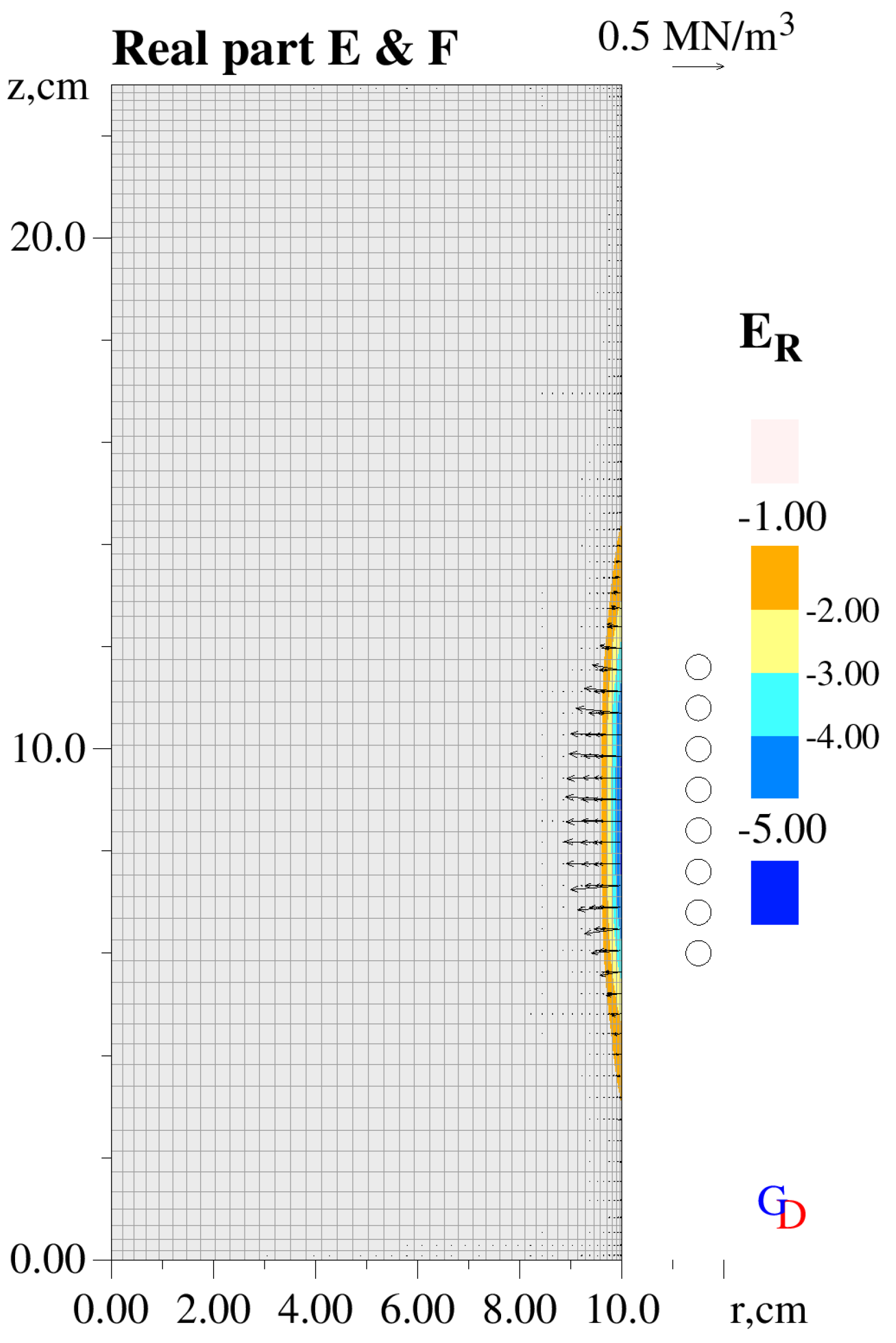
The alternating electromagnetic field produced by the AC coil with a known frequency and current amplitude induces eddy currents in the liquid metal in a thin layer by the container wall. The interaction of these currents with the magnetic field is responsible for the Lorentz force acting on the metal. Both the current and the force depend on the exact shape of the body of metal, which itself depends on the mean component of the force that causes the free surface to acquire a domelike shape resolved by specialized software [4]. Theoretically, the acoustic motion caused by the periodic component of the Lorentz force also disturbs the surface, but those oscillations of micron height can be neglected. Thus, any feedback from the acoustic field onto the electromagnetic field can be ignored, allowing the latter to be computed separately and prior to the acoustic simulation. Here, the mean deformation of the free surface is also neglected and a method consistent with CFD solvers is used [10]. Following a quasi-steady approach, it involves numerically solving partial differential equations (PDEs) for the real and imaginary components of the electric field vector E plus two extra PDEs for the real and imaginary components of an auxiliary scalar potential. The above PDEs are obtained from Maxwell’s equations of the electromagnetic field, assuming the liquid metal is a non-magnetic material with no localised electric charges—the electromagnetic induction approximation.

The computational domain only covers the electrically conducting volume of liquid metal. Boundary conditions are calculated at each iterative step for all surfaces (the ceramic crucible bottom and inner wall and the top free surface, see also Figure 1) via the Biot–Savart integral for the local values of the magnetic induction taking into account the driving and induced currents. For the axisymmetric case considered here, as the domain only covers a segment of 10 degrees, the driving and the induced electrical current segments are extended to full circles using azimuthal symmetry before Biot–Savart integration [10]. Azimuthal symmetry is also applied to the solved electric field vectors at the near and far sides of the two-dimensional sector domain [10].

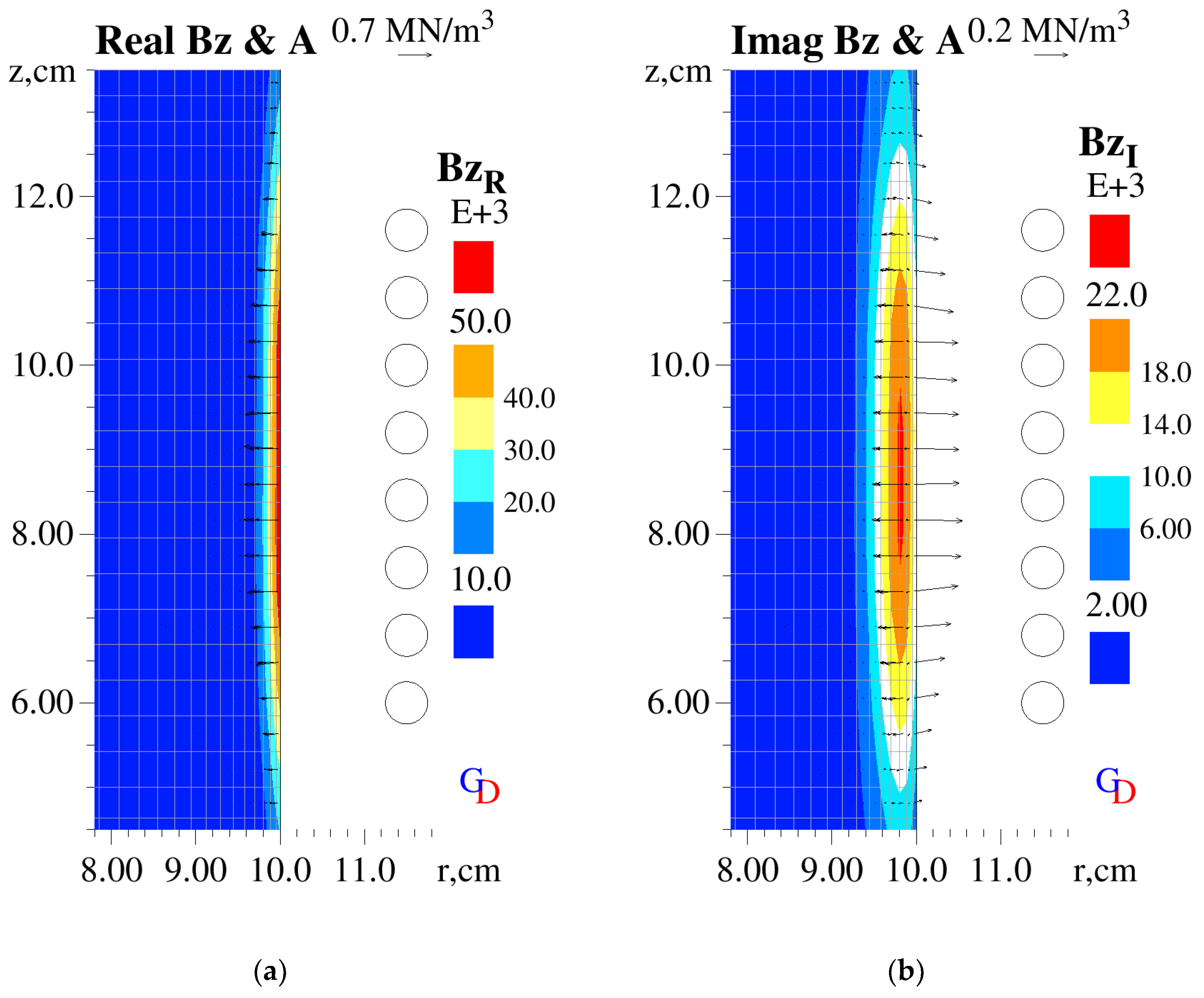
The numerical solutions are obtained on a computational mesh that is refined in the ‘skin’ layer containing the induced current (Figure 1). In a post-processing step, the mean F_M and oscillatory F_A components of the Lorentz force vector field are calculated [4] in each mesh cell:

$${\mathit{F}}_M=\frac{1}{2}\left({\mathit{J}}_R\times {\mathit{B}}_R+{\mathit{J}}_I\times {\mathit{B}}_I\right)$$

(1)

$${\mathit{F}}_A=\frac{1}{2}\sqrt{{\left({\mathit{J}}_R\times {\mathit{B}}_R-{\mathit{J}}_I\times {\mathit{B}}_I\right)}^2+{\left({\mathit{J}}_R\times {\mathit{B}}_I+{\mathit{J}}_I\times {\mathit{B}}_R\right)}^2}$$

(2)

where all imaginary parts (with subscript ‘I’) of the current density J and the magnetic induction B are 90° later in phase than the corresponding real parts (subscript R), e.g., $\mathit{B}={\mathit{B}}_R\cos \omega t+{\mathit{B}}_I\sin \omega t$ with t—time and ω [s⁻¹]—rotational frequency of the AC current. The mean force is responsible for bulk flow in the liquid volume, which may be beneficial for stirring the products of cavitation treatment, e.g., finely fractured dendrites or grain refiner particles. The oscillatory force drives the acoustic waves that cause cavitation.

For the time-dependent acoustic simulation that follows, the driving oscillatory signal is recovered from the amplitude F_A into a sinusoidal one (with a twice higher frequency) and applied as an acoustic momentum source in each cell of a new, regular Cartesian computational mesh. A mapping procedure between the two meshes is needed, and is implemented according to the following algorithm: for the centre of a CFD cell, the containing Cartesian cell is located and its indices stored; and if, due to the stepwise representation of boundaries in the acoustic module, the containing cell is not active, successive neighbours are checked and the nearest active one is selected. The solution procedure for the acoustic waves from first principles has been described elsewhere [11,12]. It is based on higher-order finite difference numerical schemes that have been optimised for accurate representation of sinusoidal functions. A characteristic of the sound propagation in liquids is the very high speed of sound compared to the fluid bulk velocity (the Mach number in liquids is always negligibly small), so all terms in the governing linearised Euler equations that have a fluid velocity component as a factor are ignored and set to zero.

The boundary conditions on all external surfaces (crucible walls and metal top free surface) are assumed ‘acoustically soft’, i.e., acoustic pressure p is fixed to zero. This assumption is justified by the fact that the acoustic impedance (the product of density and speed of sound,

Table 1. Simulated case parameters.

Parameter	Value	Unit
Crucible inner radius	100	mm
Crucible wall and bottom thickness	12	mm
Liquid aluminium depth	230	mm
Outer boundaries and top surface acoustic pressure	0	Pa
Liquid metal density	2325	kg/m3
Liquid metal speed of sound	4560	m/s
Crucible density	2000	kg/m3
Crucible speed of sound	1400	m/s
Acoustic solver mesh size	4	mm
Acoustic solver time step	1.75 × 10−7	s
Equilibrium (hydrogen) bubble radius	8	μm
Driving coil turns	8	-
Driving coil inner radius	112	mm
Driving coil outer radius	118	mm
Driving AC amplitude	650	A
Driving AC frequency	8906	Hz
Electric field error tolerance	1	mV/m
Driving acoustic source frequency	17,812	Hz
Liquid metal surface tension	0.87	N/m
Liquid metal viscosity	0.0013	Pa.s
Bubble concentration	5 × 107	m−3
Polytropic exponent	1.4	-
Ambient pressure	101,325	Pa
Smallest allowed ODE solver time step	2 × 10−13	s
Relative ODE solver error tolerance	0.0005	-
Signals monitor location radius	37	mm
Signals monitor location heights	80, 120, 160	mm
Signal RMS averaging interval	1.1	ms
Total simulated time for acoustic cavitation	0.01	s

) of the liquid metal and solid walls is orders of magnitude higher than that of the surrounding air.

Central to acoustic cavitation modelling is the representation of the bubble pulsation. When only the main, spherical mode of oscillation is considered out of the many variants investigated by numerous scientists over the years, the Keller–Miksis (3) ordinary differential equation (ODE) for the bubble radius R is used here as it provides a good balance between accuracy and complexity [13,14].

$$\begin{gathered} \left(1-\frac{\dot{R}}{c}\right)R\ddot{R}+\frac{3}{2}{\dot{R}}^2\left(1-\frac{\dot{R}}{3c}\right)=\left(1+\frac{\dot{R}}{c}\right)\frac{q}{\rho }+\frac{R}{\rho c}\frac{\partial q}{\partial t} \\ q=\left(p_0+\frac{2\sigma }{R_0}\right){\left(\frac{R_0}{R}\right)}^{3\gamma }-p_0-\frac{2\sigma }{R}-\frac{4\mu }{R}\dot{R}-p \end{gathered}$$

(3)

with p—the local acoustic time-dependent pressure, t—time, ρ and c—the density and speed of sound in the liquid, and the single and double dots over R indicating the first and second temporal derivatives. Equation (3) partially (to the first order) accounts for the liquid compressibility in its rapid radial motion in the vicinity of the bubble, as driven by the varying pressure q just outside the bubble wall; and q gives the balance of bubble pressure (depending on equilibrium radius R₀, ambient static pressure p₀ and polytropic exponent γ), surface tension σ, viscosity μ and driving acoustic pressure p. In the fully incompressible limit ($c\to \infty$), the Keller–Miksis Equation (3) reduces to the original Rayleigh–Plesset equation.

The changing bubble volume (as a function of R) determines the source term of the mass continuity equation according to the Caflisch model [15]:

$$\frac{1}{\rho c^2}\frac{\partial p}{\partial t}+\nabla ·\mathit{u}=\frac{\partial \beta }{\partial t}=\frac{\partial }{\partial t}\left(\frac{4}{3}\pi R^{3}N\right)$$

(4)

$$\rho \frac{\partial \mathit{u}}{\partial t}+\nabla p={\mathit{F}}_A\sin 2\omega t$$

(5)

u—the acoustic velocity vector, β—local bubble volume fraction, and N [m⁻³]—the local concentration of bubbles. The rate of change of β is the source term in the mass continuity equation, which represents the effect of the oscillating bubbles on the sound waves. The bubble spherical oscillation, described by R, depends on the variable local sound pressure p, thus making the interaction between sound and bubbles very tightly coupled.

Without their source terms, the system of Equations (4) and (5) describes the propagation of acoustic waves in the liquid. Since sound waves are a form fluid motion, these equations have been derived from the continuity and momentum equations of fluid flow under the assumption of the negligibly small Mach number in liquids. When these equations are solved numerically for many acoustic cycles, some numerical errors inevitably arise. Figure 2 gives an illustration of the error accumulation with the numerical implementation [12] used in this study. It shows a positive pressure pulse (with Gaussian distribution) in its initial state, and after multiple reflections at the ends of a one-dimensional computational domain. The boundary condition at the left (0) end is rigid reflection, and on the right (100)—‘sound-soft’, i.e., p = 0. An error accumulation of about 10% can be seen over 1600 acoustic cycles requiring 512,000 time steps. This number of steps is representative of what is needed to simulate an acoustic cavitation case (as shown later) over a sufficiently long time interval so that FFT analysis of monitored signals can be performed with an accuracy of about 10 Hz. The observed error is a combination of imperfections of both the numerical scheme for solving Equations (4) and (5) and the numerical boundary conditions for direct and inverted reflections, which appear in a simulated case of a vessel full of liquid.

The algorithm for the acoustic equations [12] is based on explicit time-stepping, i.e., it is subject to a CFL limit on the size of the time step depending on the density of the computational mesh, which, in turn, depends on the dimensions of the geometrical features that must be resolved; and this time step is typically in the order of 10⁻⁷ s. The numerical solution of the ODE requires about five orders of magnitude smaller time steps during bubble collapse and rebound but can revert to the acoustic time step size in the expansion phase. Here an implementation with variable time step and automatic stiffness determination that used to be available on the Intel Compiler website [16] is repeatedly called (before each acoustic time step) to cover an interval the size of the acoustic time step. During each of those intervals, the acoustic pressure p is assumed constant and fixed at its value at the beginning of the interval. This assumption is justified by the fact that the acoustic time step is already sufficiently small to resolve accurately both p and its temporal derivative. An alternative implementation where the bubble collapse is approximated in a way that avoids the need for extremely small timesteps has also provided useful results [9]. At the end of each ODE interval, the integral contribution of the Caflisch source term is calculated as

$$∆\beta =\frac{4}{3}\pi \rho c^{2}N\left(R^3-R_{old}^3\right)$$

(6)

where R is the bubble radius at the end of the current interval and R_old—at its beginning. This contribution is applied in the explicit numerical scheme [12] next time the acoustic pressure is updated according to the continuity Equation (4). The numerical solution procedures for the electromagnetic field and for the time domain propagation of acoustic waves in bubbly liquids have been incorporated into the in-house computational framework PHYSICA [17].

The cylindrical geometry of the examined case allows two-dimensional axisymmetric approximation, in which case the spiral induction coil is represented by a vertical array of rings. The parameters of the simulation are listed in Table 1. As this is an example case, the dimensions of the vessel and of the induction coil are arbitrary; the driving current and its frequency have been adjusted to achieve acoustic resonance at the lowest (in frequency) acoustic mode in the assumed geometry. The material properties of aluminium are based on various internet searches [1] and the acoustic properties of the crucible are from past research [5], the computational mesh density is chosen based on the author’s experience in past projects (the acoustic time step size then follows the CFL limit for explicit time-stepping), and the ODE solver parameters have been adjusted by trial and error based on the author’s experience. Two more parameters have been assigned arbitrary values based on past experience: the equilibrium bubble radius and the bubble concentration. When simulating a specific, practical case, these two are not known in advance and can be variable as the degassing of the melt progresses. Thus, they are treated as open parameters and can be varied to match computed results with available measurements.

3. Results

3.1. Electromagnetic Field and Forces

For the axisymmetric approximation, the calculation of the electromagnetic field and resulting forces takes about 1 min on a single workstation processor. As the dominant component of the magnetic field is vertical, it is shown in Figure 3 together with dominant components of the oscillatory part of the Lorentz force that are perpendicular to the cylindrical metal surface. The latter values are stored for use in the subsequent acoustic simulation. It can be seen that the considered values are non-zero only in the thin ‘skin’ layer of liquid metal opposite the induction coil.

3.2. Acoustic Field and Cavitation

At the beginning of the acoustic simulation, the amplitudes of the driving forces are remapped onto the regular Cartesian mesh needed for the acoustic simulation. At each time step, the real and imaginary parts of the force amplitude vectors are then used to calculate the cosine and sine contributions that drive the acoustic waves via the momentum sources in (5). Values of the acoustic pressure and of the oscillating bubble radius are recorded in selected locations and used to calculate RMS pressure, as displayed in Figure 4. The pressure contours indicate the standing-wave mode established with the highest values at the centre of the cylindrical volume (a), and the resonant growth of the acoustic pressure amplitude is interrupted when the Blake threshold of bubble pulsation is reached at about 4.5 ms (b). This is due to the really strong attenuation of the acoustic waves resulting from the elasticity of the bubbles when inertial cavitation occurs.

Although the driving oscillatory force on the metal is concentrated in the thin ‘skin’ layer of induced current (Figure 1), the highest RMS acoustic pressure is in the middle of the metal volume as this corresponds to the first acoustic resonant mode [5]. The pressure corresponding to the driving force alone is about 100 times lower than at the resonant peak, so it cannot be distinguished at the scale of Figure 4a.

An expanded image (Figure 5a) provides insight into the change of the bubble oscillation when the Blake threshold is reached: at the negative pressure half-cycle, the bubble grows more than before and high-frequency after-bounces follow every collapse at positive acoustic pressure. Figure 5b shows the frequency analysis of the monitored signals: the amplitude at the driving frequency dominates, and all higher acoustic modes appear weaker by at least one order of magnitude. This is expected under resonance and justifies the alternative approach [7] of advancing the theoretical models based on a single frequency assumption.

The combined simulation for solving Equations (3) to (5) over a time span of 10 ms (178 acoustic cycles) takes about 11 min on a 32-processor parallel workstation but the ODE implementation for (3) is not parallelised and all 1680 cells of the two-dimensional domain are processed sequentially at each acoustic time step. This time interval would ensure FFT accuracy of 100 Hz, which is not sufficient for fine tuning the driving electrical frequency. To achieve 10 Hz accuracy takes 10 times longer as the FFT resolution is inversely proportional to the sample interval. For three-dimensional domains (with many times more computational cells), the long running time may become an issue. An alternative approach to the ODE solution (with truncated bubble collapse resolution and parallel implementation) has been shown to provide useful results [9], and with that method the fuller 100 ms simulation for the examined two-dimensional case takes only 2 min.

The time domain approach to the above system of equations may have stability issues, especially with higher bubble concentration (above 10⁸ m⁻³). This is due to the increased magnitude of the source term on the right-hand side of the continuity Equation (4), which can lead to positive feedback and non-physical, unrealistic growth of the computed pressure oscillations; and then only the onset of cavitation can be predicted.

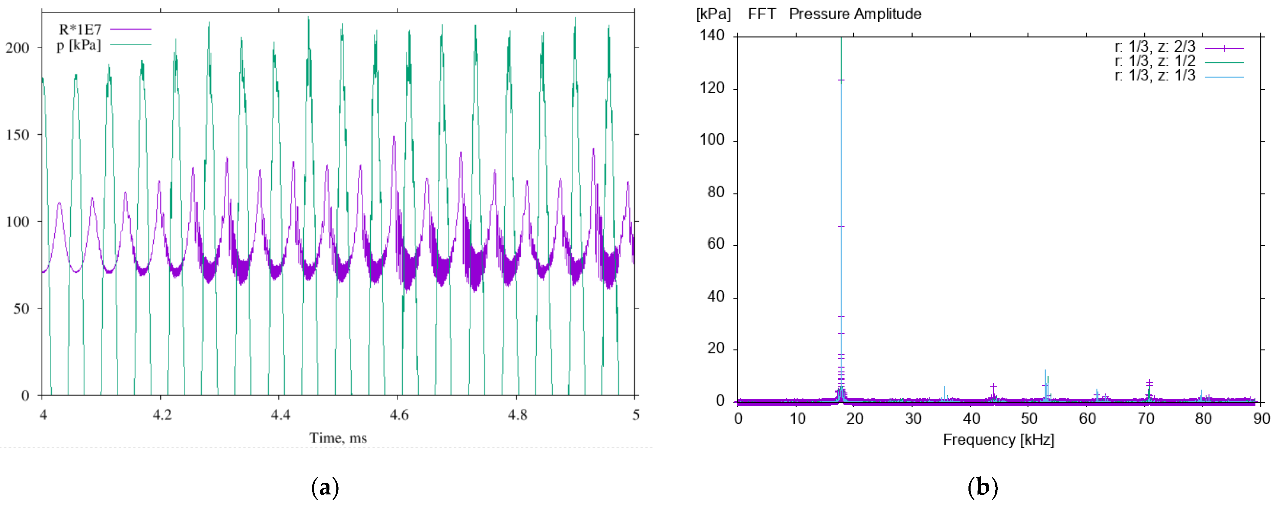
4. Discussion

The simulation results presented above highlight the mechanism of inducing and sustaining acoustic cavitation in a vessel full of liquid metal by the action of electromagnetic induction. Fine tuning of the driving AC frequency allows acoustic resonance to be initiated within the liquid volume. In the example presented in the previous section, standing waves are established at the first acoustic mode in the cylindrical geometry, which exhibits a peak of the pressure amplitude near the centre; other modes at higher frequencies can also be targeted [5], depending on the specification of the power supply to the induction coil.

The simulation results reveal the attenuation of the sound waves by the bubbles: when the acoustic pressure amplitude reaches a certain level (the Blake threshold), the oscillations of any gas bubbles contained in the liquid become violent, thus opposing further pressure growth. Some benefits of the cavitation treatment can be obtained at this level: bubbles will grow in mass by rectified diffusion from the liquid with each cycle, facilitating degassing of the melt for avoiding porosity in the final cast product. For other cavitation treatment results, e.g., primary phase dendrite fracture or grain refiner particles deagglomeration, even stronger bubble collapses may be required—then the inducing magnetic field can be amplified by increasing the driving current or the number of turns in the induction coil.

When the purpose of the simulation is to predict the acoustic spectrum of the bubbly liquid in the specified geometry, a simulated time of 0.1–0.2 s is sufficient to achieve FFT accuracy of 10 or 5 Hz needed for equipment tuning. This is at least 10 times longer than the time interval in the presented example. One option for improving the computational performance of the time-dependent method is using a truncated, approximate calculation of the bubble collapse and simultaneously parallelising the ODE solution [9]. This is suit-able for obtaining also full three-dimensional results with more than 200,000 computational cells within comfortable parameter optimisation computing time and sufficient FFT accuracy.

When the aim is to predict the degassing performance of a particular setup, a simulated time of at least 30 s would be needed to capture the bubble growth and degassing rate. The time-dependent approach in this case would follow the rectified diffusion causing the bubble growth naturally from first principles; to achieve that, a suitable model for bubble break-up after a collapse would need to be implemented and a high-performance computing cluster would be needed rather than a workstation.

5. Conclusions

The simulation sequence revealing the interaction between electromagnetic induction and acoustic cavitation has been demonstrated in an example case of a cylindrical crucible surrounded by an induction coil carrying AC current. A pseudo-steady solution of the electromagnetic field equations provides the driving force of the acoustic waves. At the next step, the modelling followed the time domain approach where the governing equations of sound propagation in the presence of oscillating and collapsing bubbles were solved with a time-dependent numerical scheme simultaneously with the ordinary differential equations for the bubble oscillation in every computational cell. The necessary software components and interfacing techniques between them have been described.

Acoustic resonance is needed for contactless electromagnetic ultrasound treatment of liquid metal, so that the acoustic pressure amplitude can reach and be sustained at a sufficiently high level for useful bubble oscillation. The acoustic behaviour of the cavitating liquid is nonlinear as the effective speed of sound changes with increasing pressure amplitude. Time-dependent modelling can predict the acoustic pressure and cavitation level at given driving frequencies. Subsequent FFT analysis can show other possible resonant frequencies, which can be confirmed by a new simulation. Fast computation allows parametric studies and optimisation to be carried out even on a desk workstation computer.