Heat Transfer Correlations for Smooth and Rough Airfoils

Abstract

Low-fidelity methods such as the Blade Element Momentum Theory frequently provide rotor aerodynamic performances. However, these methods must be coupled to databases or correlations to compute heat transfer. The literature lacks correlations to compute the average heat transfer around airfoil. The present study develops correlations for an average heat transfer over smooth and rough airfoil. The correlation coefficients were obtained from a CFD database using RANS equations and the Spalart–Allmaras turbulent model. This work studies the NACA 0009, NACA 0012, and NACA 0015 with and without the leading roughness representative of a small ice accretion. The numerical results are validated against lift and drag coefficients from the literature. The heat transfer at the stagnation point compares well with the experimental results. The database indicates a negligible dependency on airfoil thickness. The work presents two correlations from the database analysis: one for the smooth airfoils and one for the rough airfoils. For the zero lift coefficient, the average Nusselt number is maximum. This increases with $R{e}^{0.636}$ for the smooth surface and with $R{e}^{0.85}$ for the rough surface. As the lift increases, the average Nusselt is reduced by values proportional to the square of the lift coefficient for the smooth surface, while it is reduced by values proportional to $Re$ and the square of the lift coefficient for the rough surface.

1. Introduction

Aircraft and helicopters need ice protection systems (IPSs), such as anti-icing or de-icing systems, to safely fly through supercooled water droplets in clouds [1]. Thermal melting is the most common method of preventing ice buildup on critical surfaces. The main goal for IPSs is to use the lowest power while ensuring safe ice removal for various atmospheric conditions [2]. The IPS should remove ice accretion to avoid aerodynamic performance degradation without exceeding the critical temperature of the materials, even if the IPS operates outside in-flight icing conditions. Experimental methods [3,4] or computational fluid dynamics (CFD) methods [5,6,7], coupled with reduced-order modeling and optimization methods provide insightful information for the detailed design. However, these high-fidelity tools are expensive to use in the early development phases when several aircraft or helicopter configurations are evaluated. A medium fidelity method such as the vortex lattice method, (VLM) coupled with a 2D viscous database, is computationally less expensive and enables aircraft icing studies [8].

Researchers have coupled low-fidelity methods, such as Blade Element Momentum Theory (BEMT), or medium fidelity methods, such as the VLM, and airfoil lookup tables or correlations to estimate aerodynamic forces, performance degradation or heat transfer. VLM and a drag correlation based on airfoil experimental data enable the computationally efficient calculation of the vibration of helicopter rotors [9]. The nonlinear unsteady VLM coupled to 2D RANS or empirical databases adequately predicts helicopter rotor aerodynamics in hover [10]. Nonlinear VLM coupled to 2.5D RANS sectional data allows the prediction of the maximum lift coefficient for a 3D swept wing [11]. The results agree reasonably well with 3D RANS solution, and the proposed approach is well suited for preliminary design. A model for predicting the torque for a rotor under icing conditions is proposed based on the BEMT [12,13] and a correlation for airfoil performance degradation in an icing environment [14]. Samad et al. [15] coupled the VLM with a 2D RANS database to compute lift and drag. The effective angle of attack and the Reynolds number are determined at each radial position of the blade. Then, the average heat transfer coefficients are computed using a correlation based on a RANS database for an airfoil under fully turbulent conditions [16].

The correlations for the aerodynamic forces on 2D airfoil often related the lift coefficient, $c_l$, to the angle of attack $\alpha$, and the drag coefficient $c_d$ to $c_l$. For a typical airfoil at high Reynolds numbers, $c_l$ linearly evolves with $\alpha$ until the flow separates from the surface, close to the stall angle [17]. The maximum lift coefficient and the aerodynamic forces after the stall angle depend on many parameters, the Reynolds number and the airfoil shape included among them [18]. Researchers used experimental and RANS databases to build correlation for both $c_l$ and $c_d$ at the post-stall angle [19]. Before the stall angle, Hoerner [20] suggests that $c_d$ is a function of the square of the lift coefficient. Usually, $c_d$ has a minimum value $c_{d,min}$ for $-2^{\circ }<\alpha <2^{\circ }$ [21]. At this minimum drag value, the lift coefficient is $c_{l,mind}$, such that

$$c_d=c_{d,min}+A{(c_l-c_{l,mind})}^2$$

Recent research has suggested a novel estimation method for $c_{d,min}$ over smooth airfoil based on an extensive RANS database, including 40 airfoil shapes [22]. Gotten et al. decomposed $c_{d,min}$ in the friction drag and the pressure drag, both functions of the airfoil shape parameters. This estimation method extends the Reynolds range of the validity of the previous correlations.

Most correlations relate the heat transfer to the Reynolds number, $Re$, and the Prandtl number, $Pr$. For well-studied geometries such as a flat plate, the Nusselt number $Nu$ is related to $Re$ and $Pr$ [23]. Separate correlations model the laminar or turbulent flows, but Lienhard [24] suggested approximations that also include the transitional flows. For a cylinder in cross flow, the $Nu$ [25] or the Frossling number $Fr=Nu/\sqrt{Re}$ [26] correlate with $Re$ and $Pr$. For ice-roughened surfaces, limited data are available, but some researchers use $Fr$ instead of $Nu$ [27].

The literature suggests heat transfer correlations for heat exchanger analysis. In particular, recent studies used vortex generators, geometries that share some analogy with wings, to enhance the heat transfer in tubes. The Dittus–Boelter equation, $Nu=0.023R{e}^{0.8}P{r}^{0.4}$, is modified to consider the geometry, the angle of attack, and the spacing of the vortex generators. The correlation coefficients are obtained using the least-square regression method with experimental data [28,29]. Heat transfer enhancement by vortex generators was also numerically studied using CFD [30] data. Instead of correlations, artificial neural network models have been used for the performance prediction and optimization of complex heat exchanger geometries [31].

Compared to flat plates and cylinders, heat transfer correlations for airfoil have a minimum of two additional parameters: the airfoil shape and the angle of attack, $\alpha$. Fewer experimental data and correlations are publicly available for the convective heat transfer around airfoil. Most notably, the works of [32,33] studied the heat transfer coefficient in the leading edge area of an NACA0012 with smooth and rough surfaces, for $-6^{\circ }<\alpha <8^{\circ }$. The local $Fr$ over the smooth surface was independent of $Re$ close to the stagnation point. The rough surfaces consisted of 2 mm diameter hemispheres arranged in four patterns. Dukhan et al. experimentally measured the $Fr$ in the first $10\%$ of an NACA 00012 with mildly rough glaze and rough glaze ice with horns [34]. At $\alpha =0^{\circ }$, the $Fr$ at stagnation point is a quadratic function of $Re$. Downstream from the stagnation point, the local $Fr$ is a polynomial function of the distance along the airfoil. The polynomial constant values vary with $Re$. When ice accretes on an airfoil, the local $Fr$ increases in time as the ice roughness grows [35]. Average heat transfer correlations for NACA0010 [36] and the NACA 63-421 [37] are proposed based on experimental results. Both correlations relate the average Nusselt $\overline{Nu}$ to $Re$. Further works expand the correlation for NACA 63-421 to include the effects of $\alpha$ on $\overline{Nu}$ based on the experimental measurements between $0^{\circ }<\alpha <{25}^{\circ }$ [38].

Instead of experiments, Samad et al. [15] used CFD to build a correlation for the $Fr$ number as a function of $Re$ and $\alpha$ for the NACA 0012 under fully turbulent flow conditions. They further improved the correlation to predict the post stall heat transfer using a cubic variation with $\alpha$ [16]. Using experimental results on a rotor, Ref. [39] proposed correlations to include the effects of water spray and the presence of an ice layer for $\alpha =6^{\circ }$.

The design of IPS requires the heat loss by the airfoil to the cold airflow. The BEMT and the unsteady VLM enable the quick prediction of the aerodynamic forces and the average heat transfer if they are coupled with correlations to include viscous effects. However, correlations for average heat transfer are only available for three airfoils with smooth surfaces at $Re<3\times {10}^6$. The present study partially addresses this gap by studying the effects of the airfoil thickness, the lift coefficient and the roughness on symmetric airfoil for $Re<6\times {10}^6$. The study develops correlations for the average heat transfer over smooth and rough airfoil. A RANS database for aerodynamic flows over symmetric airfoils helps build the correlations. The study focuses on heat transfer before the stall for fully turbulent flow in the range $0.625\times {10}^6\le Re\le 6.0\times {10}^6$. Three airfoil thicknesses to cord ratios, $t/c=0.09$, $0.12$, and $0.15$, assess the result sensitivity to the thickness. The addition of leading edge roughness models the ice accretion effects. First, the paper presents the RANS model used together with the meshes and the proposed average heat transfer function. Second, the lift, drag, and heat transfer from the literature validate the RANS model predictions. Then, the database is verified and used to suggest two heat transfer correlations: one for the smooth airfoils, and one for the rough airfoils.

2. Materials and Methods

In the context of rotor aerodynamics, the work assumes that each blade section acts as a quasi-2D airfoil to produce aerodynamic forces and heat transfer, and thus 3D effects such as wing tip vortices are not included. The flow of air is compressible and fully turbulent, and no laminar boundary layer region exists on airfoil. The heat transfer by radiation is neglected. The conduction and the thermal inertia in the airfoil skin are negligible as the temperature is constant in both time and space.

The heat transfer coefficients over three airfoils were obtained using CFD. The airfoils were selected to study the results’ sensitivity to the thickness-to-cord ratio. The symmetric NACA 0009, NACA 0012, and NACA 0015 have a maximum thickness-to-cord ratio, $t/c$, of $0.09$, $0.12$ and $0.15$, respectively, located at $x/c=0.3$, as shown in Figure 1. The surface is either smooth or rough to model the effects of small ice accretion. The roughness covers the leading edge region, in the first $8\%$ of the cord. The ice accretion depends on atmospheric conditions and can sometimes extend up to $15\%$ of the cord. The present choice of the first $8\%$ follows from previous experimental works [40]. For this study, $\alpha$ goes from $0^{\circ }$ up to the stall angle.

The compressible RANS equations model the airflow around the airfoil [41]. The air is considered to be a perfect gas, with a specific gas constant $R=287.058J/kgK$ and specific heat ratio coefficients at a constant pressure and volume $\gamma =c_p/c_v=1.4$. The Sutherland formula gives the dynamic viscosity $\mu$ for air as a function of temperature T

$$\mu =\frac{1.45\times {10}^{-5}{T}^{3/2}}{T+110}.$$

(1)

The thermal conductivity k is obtained from $Pr$

$$k=\frac{c_p\mu }{Pr}.$$

(2)

The Prandtl number has a constant value of $0.72$. The effects of relative humidity on the air properties are neglected [42].

The flow is fully turbulent, for both smooth and rough airfoils. The Spalart–Allmaras turbulent model (SA) is used for the smooth surface [43]. The SA model is commonly used in aeronautics to model attached flow as it gives satisfactory predictions for lift and drag [41]. The Boeing method corrects the SA model (SA-rough) to predict the flow over rough walls [44]. This model accounts for roughness effects on the wall shear stress with the equivalent sand grain roughness, $h_s$, but an additional correction is needed for the heat transfer prediction. The two parameters of the Prandtl correction model [45] add the function $\Delta P{r}_t$ to the otherwise constant turbulent Prandtl number, $P{r}_t=0.9$. Briefly, the correction $\Delta P{r}_t$ depends on $h_s$ and the physical roughness height h. For a roughness Reynolds number $R{e}_s$ above 70, the correction is

$$\begin{array}{ccc}\hfill \Delta P{r}_t& =& 0.136\frac{R{e}_s^{0.45}P{r}^{0.8}}{1.92},\hfill \end{array}$$

(3)

$$\begin{array}{ccc}\hfill R{e}_s& =& \frac{\rho u_{\tau }{h}_s}{\mu },\hfill \end{array}$$

(4)

$$\begin{array}{ccc}\hfill u_{\tau }& =& \sqrt{{\tau }_w/\rho }.\hfill \end{array}$$

(5)

At the wall, the SA-rough model predicts a non-zero eddy viscosity ${\mu }_t$, and therefore the heat flux at the wall, $q_w$, is

$$\begin{array}{ccc}\hfill q_w& =& -(k+k_t){\left(\frac{\partial T}{\partial y}\right)}_w,\hfill \end{array}$$

(6)

$$\begin{array}{ccc}\hfill k_t& =& \frac{c_p{\mu }_t}{P{r}_t+\Delta P{r}_t}.\hfill \end{array}$$

(7)

where ${\left(\frac{\partial T}{\partial y}\right)}_w$ is the temperature gradient at the wall. Over smooth surfaces, the SA model imposes ${\mu }_t=0$ and $\Delta P{r}_t=0$.

The local Nusselt number is defined based on the airfoil cord $c=$ 1 m and the recovery temperature at freestream $T_t$

$$\begin{array}{ccc}\hfill Nu& =& \frac{q_{w}c}{(T_w-T_t)},\hfill \end{array}$$

(8)

$$\begin{array}{ccc}\hfill T_t& =& T_{\infty }(1+P{r}^{1/3}0.5(\gamma -1)M{a}^2).\hfill \end{array}$$

(9)

where $Ma$ and $T_{\infty }$ are the farfield Mach number and temperature. An average Nusselt number $\overline{Nu}$ over the airfoil wet surface s can also be defined, such that

$$\begin{array}{ccc}\hfill \overline{Q}& =& \frac{\int q_{w}ds}{s},\hfill \end{array}$$

(10)

$$\begin{array}{ccc}\hfill \overline{Nu}& =& \frac{\overline{Q}c}{(T_w-T_t)},\hfill \end{array}$$

(11)

for a constant wall temperature $T_w=300K$.

The 2D computational domain consists of a circle of radius $100c$ with the airfoil leading edge located at the center, as illustrated in Figure 2. Riemann boundary conditions are imposed at the farfield boundary. The Mach number is $Ma=0.2$ and the temperature is $T_{\infty }=268.15K$. The static pressure at farfield $P_{\infty }$ set the density $\rho =P_{\infty }/R{T}_{\infty }$ and the Reynolds numbers, $Re=\rho V_{\infty }c/\mu$. The turbulence model variable $\tilde{\nu }$ is set to three times the kinematic viscosity at farfield. At the airfoil wall, a no-slip boundary condition is imposed together with a constant temperature. For the rough leading edge, the standard leading-edge roughness consists of carborundum grains applied to the surface of the model [40]. In [40], 0.279 mm carborundum grains are applied to a $c=$ 0.6096 m airfoil. The equivalent sand grain roughness is $h_s/c=0.001$ and the roughness height is $h/c=0.00458$, corresponding to the small ice accretions between deicing cycles.

Mixed meshes discretize the computational domain. The mesh generator Gmsh [46] builds rectangular elements with a growth ratio of $1.15$ for a normal surface distance lower than $0.02c$ and triangular elements farther away. For each airfoil, three meshes are constructed to enable a grid convergence study. Figure 3 shows a close-up view of the airfoil leading edge for the NACA 0012 medium mesh. For the coarse, medium and fine meshes, the first node above the surface is located at $3.5\times {10}^{-6}$ m, $2.5\times {10}^{-6}$ m and $1.8\times {10}^{-6}$ m. At $Re=6\times {10}^6$, this corresponds to maximum dimensionless wall distances $y^{+}=0.48$, $0.35$, and $0.25$ above the smooth surface, respectively. For the rough surface and the medium mesh, $y^{+}=0.7$. The number of nodes on the airfoil surface is approximately 400, 560, and 780 with a smaller node spacing close to the leading edge and the trailing edge. For the medium mesh in Figure 3, at $Re=6\times {10}^6$, $x^{+}\approx 70$ is close to the leading edge.

The steady RANS equations are solved with a modified version of the finite volume code SU2 version 6.2 [47]. The modifications implement the SA-rough model and the turbulent Prandtl number correction for flow over the rough surface, as validated in [45]. The RANS and SA equations are discretized over the mesh using a cell-vertex scheme with median dual control volumes. The space numerical integration uses the Roe scheme for the RANS inviscid terms [48]. To reach second-order accuracy, the MUSCL scheme is used with a Venkatakrishnan–Wang slope-limiting method [49]. For the viscous terms, the gradients are computed using the Green–Gauss theorem [41]. The steady-state solution is iteratively reached using an implicit time stepping scheme. An Euler implicit time integration method is used for the flow equations with an adaptive Courant–Friedrichs–Lewy (CFL) number, with $0.5<CFL<10$. The flexible generalized minimal residual method, FGMRES, solves the resulting linear system of equations using a LU-SGS preconditioning [47]. The iterations stop when the residual of the density equation is below ${10}^{-11}$.

The grid convergence method (GCI) is applied [50] to study the effects of the grid refinement on $\overline{Nu}$. The maximum GCI for the three smooth airfoils at $\alpha =0^{\circ }$, ${10}^{\circ }$, and ${15}^{\circ }$ is $0.18\%$. For the three rough airfoils, at $\alpha =0^{\circ }$, $5^{\circ }$, and $8^{\circ }$, the maximum GCI is $2\%$. This is higher than for the smooth airfoil, but still acceptable to build a database for correlations. The GCi is a measure of the grid-induced errors. At $2\%$, it is lower than the error induced by the turbulence model choice between $\approx 3\%$ and $5\%$ according to [16].

This work assumes that $\overline{Nu}$ is a function of $Re$, $c_l$, and $Pr$

$$\overline{Nu}=(AR{e}^B+C{c}_l^2)P{r}^{1/3}$$

(12)

for the attached and mildly separated flow. The $Pr$ dependency is assumed for compatibility with previous correlations.

The database contains 360 CFD simulations. The simulations are run at five Reynolds numbers $Re=0.625\times {10}^6$, $1.25\times {10}^6$, $2.5\times {10}^6$, $4.0\times {10}^6$, $5.0\times {10}^6$, and $6.0\times {10}^6$. The $\alpha$ range is limited by the stall angle, reached at lower values for the rough airfoils. For the smooth airfoils, $\alpha =0^{\circ }$, $2^{\circ }$, $4^{\circ }$, $6^{\circ }$, $8^{\circ }$, ${10}^{\circ }$, ${12}^{\circ }$, ${13}^{\circ }$, ${14}^{\circ }$, and ${15}^{\circ }$. For the rough airfoils, $\alpha =0^{\circ }$, $2^{\circ }$, $4^{\circ }$, $6^{\circ }$, $8^{\circ }$, $9^{\circ }$, ${10}^{\circ }$, ${11}^{\circ }$, ${12}^{\circ }$, and ${13}^{\circ }$. The correlation coefficients A, B, and C are not sensitive to the three thickness ratios $t/c$ selected.

3. Results

The coefficients A, B, and C are determined by fitting the nonlinear regression model Equation (12) to the CFD dataset [51]. The CFD results are first validated against experimental lift and drag coefficients for the three airfoils. The Nusselt number predictions are validated against experimental data for the NACA 0012. Then, the heat transfer results are verified at $\alpha =0^{\circ }$ over the Reynolds range and at $Re=6\times {10}^6$ over the $\alpha$ range. Finally, $\overline{Nu}$ is correlated to $Re$ and $c_l$ for smooth and rough surfaces.

3.1. Validation

With a maximum GCI around $2\%$, the medium mesh precision is sufficient to build average heat transfer correlations. The CFD results for the NACA 0009 and NACA 0012 on the medium mesh are validated against experimental lift and drag coefficients from [40,52]. Although the compressible RANS equations are solved, the compressible effects are essentially negligible. The CFD Mach number is $0.2$ and the Reynolds number is $Re=6\times {10}^6$. Figure 4 shows the $c_l$ evolution with $\alpha$. For the NACA 0012, two sets of experimental data are plotted. The $c_l$ linearly increases with $\alpha$ for both the NACA 0009 and NACA 0012 until around $\alpha ={12}^{\circ }$. At $\alpha ={13}^{\circ }$, the experimental results for the NACA 0009 show a decrease in $c_l$, whereas the $c_l$ predicted by the SA model keeps increasing, but not linearly. For the NACA 0012 experimental results, the maximum lift coefficient is reached around $\alpha \approx {16}^{\circ }$, above the maximum $\alpha ={15}^{\circ }$ for the CFD simulation.

Figure 4 also compares the $c_d$ as a function of $c_l$. For NACA 0012, $c_d$ from [52] experiments, obtained by tripping the boundary layer at the airfoil leading, is closer to the CFD results than the untripped Abott results for $c_l<1$. The fully turbulent CFD results for both airfoils are close until $c_l\approx 1.2$. Then, the predicted $c_d$ increases faster for the NACA 0009, most probably because the stall occurs at $\alpha ={13}^{\circ }$. Note that Abbott results do not include $c_d$ values above the stall angle.

For the NACA 0015 geometry, the SA results are compared to the experimental results [53] and numerical results [54] in Figure 5. The Reynolds number is $Re=1.6\times {10}^6$. For the SA model, the Mach number is kept at $0.2$. The SA model results agree well with the SST turbulence model results. Both numerical results fail to predict the stall angle and maximum lift coefficient, but closely follow the experiments for $\alpha <{12}^{\circ }$. Although the experimental results are for untripped flow, the predicted drag coefficients $c_d$ in Figure 5 are only slightly above the measurements before the stall angle, $\alpha <{15}^{\circ }$. The SST and SA results provide similar drag predictions.

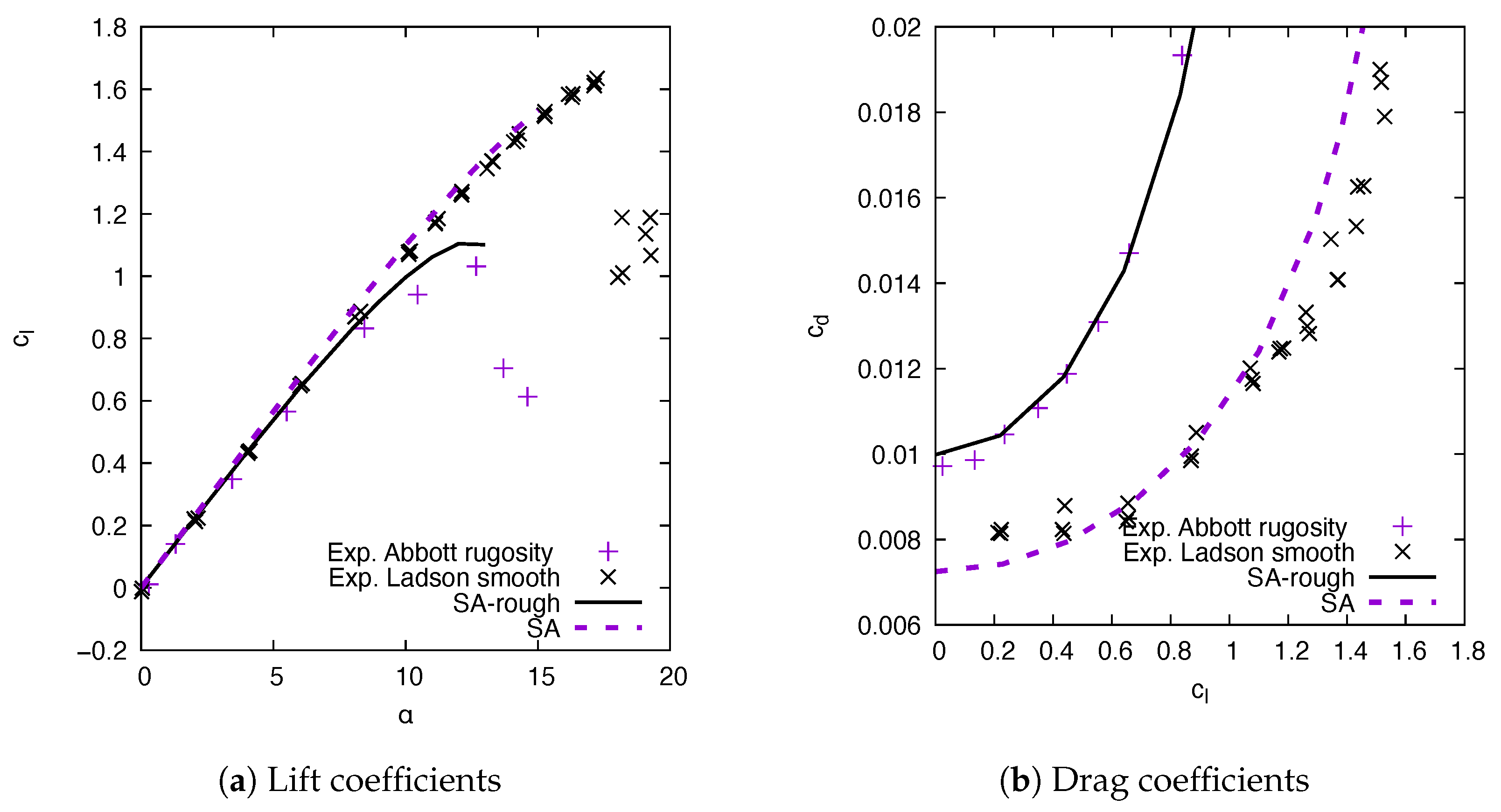
For the rough results, the equivalent sand grain roughness is $h_s/c=0.001$ and the roughness height is $h/c=0.00458$, approximately corresponding to the experimental grit 60 size roughness used on the NACA 0012 airfoil of $c=0.6096$ m [40]. Figure 6a,b compare the predicted $c_l$ and $c_d$ with the experimental results of [40] for the NACA 0012 with roughness at $Re=6\times {10}^6$. The results for the smooth NACA 0012 are also plotted to ease the comparison. The reduction in the maximum lift coefficient is well predicted by the SA-rough model. The increase in the drag coefficient is similar to that observed experimentally, with a maximum discrepancy of approximately $3\%$.

Almost no data are available for the validation of the CFD average heat transfer prediction over an airfoil. The SA-rough model coupled with the thermal Prandtl correction was previously validated against flat plate results [45], or flow with curvature [55]. No experimental data for average heat transfer over the airfoils at high Reynolds number and fully turbulent flow are available. However, the heat transfer at the NACA 0012 stagnation point is compared with the experiments. Figure 7 shows the predicted heat transfer for both the SA and SA-rough model at the leading edge as a function of $Re$. The angle of attack is $\alpha =0$. In [56], a correlation based on the heat transfer measurement at the airfoil leading edge in the IRT wind tunnel is given, as $Nu=6.818R{e}^{0.472}$. The correlation is valid for smooth surfaces, and for the Reynolds range of the experiment, $1.2\times {10}^6<Re<4.5\times {10}^6$. The SA model prediction closely follows the experimental results. The SA-rough results are also plotted to show that $Nu$ increases with surface roughness at a lower Reynolds number, approximately $8\%$ of increases at $Re=2.5\times {10}^6$. For $Re\ge 4\times {10}^6$, the heat transfer at the leading edge is unaffected by the roughness.

3.2. Database Verification

Previous experiments with airfoils at a lower $Re$ [36,37] and correlations for heat transfer in the turbulent boundary layer [23] predict that $\overline{Nu}$ should increase with $Re$. Figure 8 shows that $\overline{Nu}$ has a function of $Re$ for the three airfoils. Although the roughness height $h_s$ is constant, the roughness Reynolds number, $R{e}_s$ increases from $\approx 50$ at $Re=0.625\times {10}^6$, to $\approx 500$ at $Re=6\times {10}^6$. According to [57], the roughness regime is transitionally rough for $Re=0.625\times {10}^6$ and fully rough for all the others $Re$.

At $\alpha =0^{\circ }$, the results for rough airfoils increase faster than the results for smooth airfoils. The effects of airfoil thickness $t/c=9\%$, $12\%$, and $15\%$ on $\overline{Nu}$ are small once the total heat flux is divided by the respective wet surface $s=2.02c$, $2.04c$, and $2.06c$. For comparisons, the correlation for the turbulent heat transfer over a flat plate of length c

$$\overline{Nu}=(0.037R{e}^{0.8}-871)P{r}^{0.333}$$

is also plotted [23]. The curve for the flat plate gets closer to the smooth airfoil results as $Re$ increases. The discrepancy between the rough and smooth results increases with $Re$, reaching a maximum value of $\approx 9\%$ for $Re=6\times {10}^6$. This indicates that the Reynolds exponent in Equation (12) must be different for rough and smooth surfaces.

The heat transfer locally increases above the roughness and reduces to smooth values downstream of the first $0.08c$. The fraction of the surface with roughness, $s_r$, changes with increasing airfoil thickness, such that $s_r=0.089s$, $0.094s$, and $0.099s$. $\overline{Nu}$ blurs the effects of roughness. To emphasize the roughness effects, Figure 9 shows that the Nusselt number averaged over the first $0.08c$

$$\begin{array}{ccc}\hfill \overline{Q_r}& =& \frac{\int q_{w}ds}{s_r},\hfill \end{array}$$

(13)

$$\begin{array}{ccc}\hfill \overline{N{u}_r}& =& \frac{\overline{Q_r}c}{(T_w-T_t)}.\hfill \end{array}$$

(14)

$\overline{N{u}_r}$ is significantly higher in the leading edge area than for the complete airfoil, with a maximum value for the rough surface of $2.0\times {10}^5$ compared to $0.9\times {10}^5$. The results are more sensitive to the roughness than to the airfoil thickness. As in Figure 8, the discrepancy between the smooth and rough results increase with $Re$. At $Re=0.625\times {10}^6$, $\overline{N{u}_r}$ is $\approx 13\%$ higher for the rough surface. At $Re=6\times {10}^6$, $\overline{N{u}_r}$ is $\approx 80\%$ higher for the rough surface. This confirms the need for a different correlation for the flow over the rough surface. The heat transfer decreases as the airfoil thickness increases. However, the effect of the airfoil thickness at $\alpha =0^{\circ }$ is negligible, being at least an order of magnitude smaller than the effects of $Re$ and roughness.

For symmetric airfoil, $\overline{Nu}$ should be maximum when $\alpha =0^{\circ }$. As $c_l$ increases, the stagnation point moves towards the pressure side and the curvilinear distance from the stagnation point to the trailing edge increases on the suction side. The thermal boundary layer becomes thicker on the suction side; thus, the heat transfer is reduced. This is observed on Figure 10a for the three airfoils at $Re=6\times {10}^6$ for both the smooth and rough surface. $\overline{Nu}$ for the NACA 0009 decreases faster with the lift coefficient than $\overline{Nu}$ for the thicker airfoils. Figure 10b shows that the predicted maximum $c_l$ for the rough airfoil is approximately $0.95$ for the NACA 0009, which is below the maximum $c_l\approx 1.1$ for the thicker airfoils. For these airfoils, the flow separation eventually starts at the trailing edge before the maximum lift coefficient is reached. In the separation area, the heat transfer is further reduced. As a consequence, $\overline{Nu}$ for the rough airfoils are lower than for the smooth airfoils, for $c_l>0.9$ or $c_l>1.0$ depending on the airfoil thickness. $\overline{Nu}$ shows a stronger dependency on $c_l$ and roughness than on the airfoil thickness.

3.3. Correlations

The average Nusselt numbers for the three smooth airfoils are gathered together to obtain the correlation coefficients. The coefficients are estimated using the Levenberg–Marquardt nonlinear least squares algorithm [51] such that the sum of the squares of the deviations is minimized. The coefficients do not significantly change if the airfoil thicknesses are considered separately. The following correlation fits the data with a coefficient of determination $R^2=0.998$

$$\overline{Nu}=(0.0289R{e}^{0.81}-257c_l^2)P{r}^{1/3}.$$

(15)

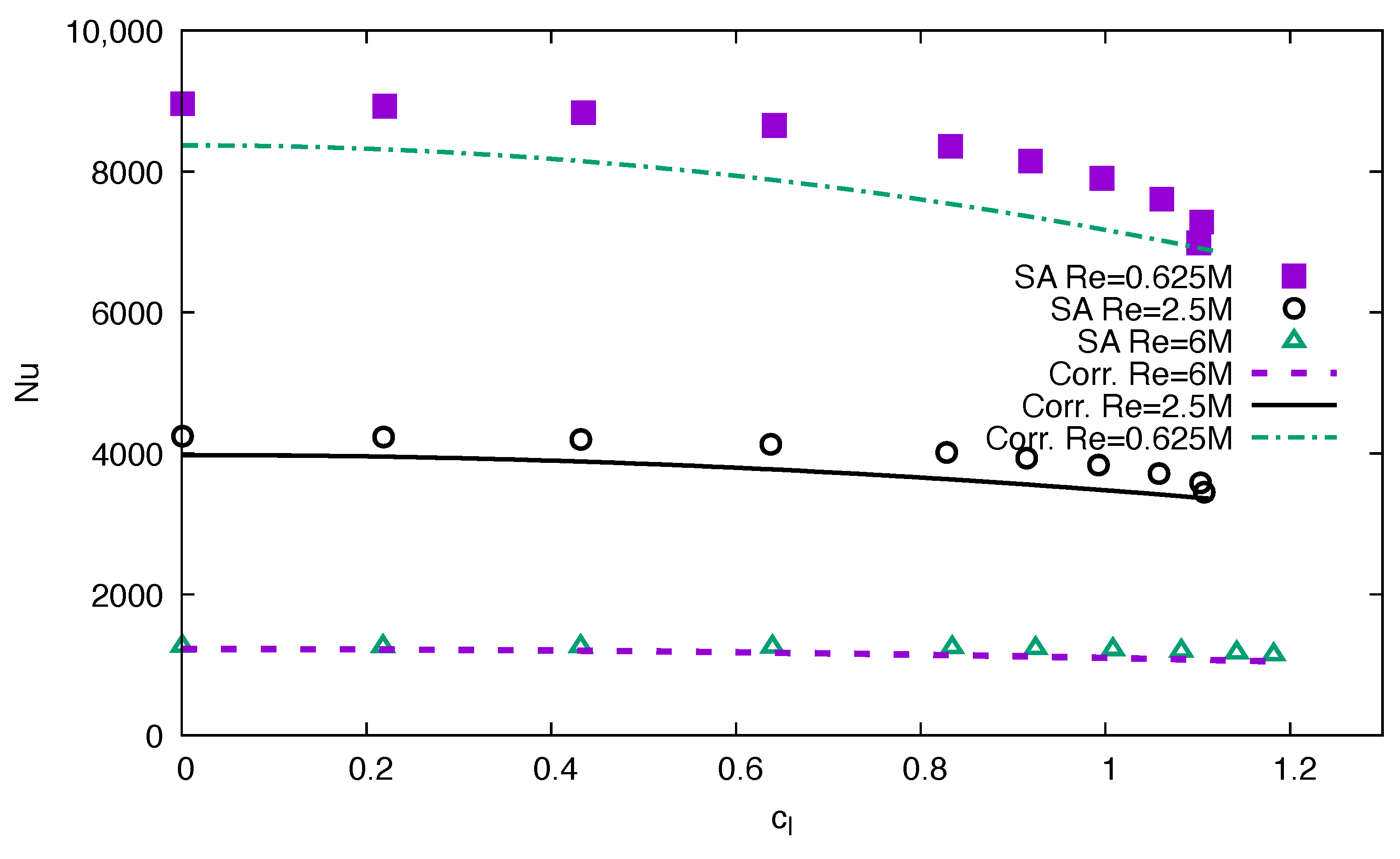
The correlation predictions are compared to the CFD data for the smooth NACA 0012 airfoil on Figure 11. The $\overline{Nu}$ values are plotted at three Reynolds numbers, $Re=0.625\times {10}^6$, $2.5\times {10}^6$, and $6\times {10}^6$ as a function of $c_l$. The maximum error on $\overline{Nu}$ is $\pm 250$, and it occurs for the lowest $Re$ number and $c_l>1.1$.

Similarly, the average Nusselt numbers for the rough airfoils are gathered together. Unlike the smooth correlation Equation (15), coefficient C in front of $c_l^2$ must increases linearly with $Re$ to obtain a coefficient of determination $R^2=0.998$

$$\overline{Nu}=(0.0162R{e}^{0.85}-(2.23\times {10}^{-4}Re)c_l^2)P{r}^{1/3}.$$

(16)

For the rough airfoils, $\overline{Nu}$ decreases faster with the lift coefficient at a higher $Re$, as shown in Figure 12. At $Re=1.25\times {10}^6$, the rate of decrease with $c_l^2$ is $C=279$, close to the $C=257$ value in the Equation (15). For $Re>1.25\times {10}^6$, $\overline{Nu}$ is more sensitive to the lift coefficient for the rough airfoils than for the smooth airfoils.

4. Discussion

This work proposes two correlations to predict the average heat transfer over an airfoil. The correlations are the results of a nonlinear curve fit of a CFD database. The RANS equations and the SA turbulence model poorly predict large flow separations. Hence, the database focuses on fully turbulent flow around the airfoil before the stall angle. The database assumes that the average heat transfer depends on four parameters, $\overline{Nu}$$(Re,\alpha ,h_s,t/c)$. The most important parameter is $Re$. The analysis shows that the correlation coefficients are mostly insensitive to $t/c$ in the studied range, $0.09\le t/c\le 0.15$. To the best of our knowledge, this is the first time the sensitivity of the heat transfer to $t/c$ has been investigated. The average discrepancy between the $\overline{Nu}$ values determined from CFD simulations and the values calculated with the correlation is $3\%$, with discrepancies reaching $\approx 20\%$ close to the maximum $c_l$ for the lowest $Re$.

The originality of the proposed correlations comes from the fact that they cover Reynolds numbers up to $6\times {10}^6$, relate the average heat transfer coefficient to the lift coefficient, and take into account the surface roughness. Literature correlations for airfoil in free stream flow are summarized in

Table 1. Correlations from the literature.

Airfoil	$\overline{\mathit{Nu}}$	$\mathit{Re}$	$\mathit{\alpha }$
NACA 0010 [36]	$0.0000422R{e}^{1.3065}P{r}^{1/3}$	$5\times {10}^5\le Re<8.1\times {10}^5$	$\alpha =0^{\circ }$
NACA 0010 [36]	$0.0206R{e}^{0.8356}P{r}^{1/3}$	$Re<5\times {10}^5$	$\alpha =0^{\circ }$
NACA 63-421 [38]	$0.0943(0.75+0.017\alpha )R{e}^{0.636}P{r}^{1/3}$	$5\times {10}^5\le Re<1.1\times {10}^6$	$0^{\circ }<\alpha <{25}^{\circ }$
NACA 63-421 [38]	$2.482(0.75+0.013\alpha )R{e}^{0.389}P{r}^{1/3}$	$Re<5\times {10}^5$	$0^{\circ }<\alpha <{25}^{\circ }$
NACA 0012 [15]	$0.023(1-0.389\alpha -0.678{\alpha }^2)R{e}^{0.830}P{r}^{1/3}$	$2\times {10}^5\le Re<3.0\times {10}^6$	$0^{\circ }<\alpha <{30}^{\circ }$

. They are mostly for laminar or transitional flow [36] or low Reynolds number turbulent flows, $Re<3\times {10}^6$ [15,38]. Some correlations in the related literature correct the heat transfer by a factor proportional to the angle of attack [15,38], but not the lift coefficients. Furthermore, the present study is the first to suggest that the NACA 0009, NACA 0012, and NACA 0015 could use the same correlation if the average is based on the wet surface.

The correlation results from Table 1 are compared against Equation (15) results for a smooth NACA 0012 at $\alpha =0^{\circ }$ in Figure 13. The Equation (15) results agree with [15,36] but extend the range of validity to $Re=6\times {10}^6$. The results of [38] for a NACA 63-421 are noticeably lower, around $\overline{Nu}=500$ at $Re=1\times {10}^6$ instead of $\overline{Nu}\approx 2000$. This is in line with their measured value at the stagnation point. At the stagnation point, the local $Nu\approx 900$ for $Re=1.037\times {10}^6$, and $\alpha =0^{\circ }$ (and $c_l>0$), approximately five times less than that measured for an NACA 0012. As $Re$ increases, the flat plate correlation results get closer to Equation (15).

The maximum $\overline{Nu}$ occurs for $\alpha =0^{\circ }$. For the smooth airfoils at $Re>2.5\times {10}^6$, the average heat transfer is only slightly above the one predicted by a correlation for a turbulent flow over a flat plate. As $\alpha$ increases, the lift coefficient increases and $\overline{Nu}$ decreases. For example, a $10\%$ decrease is observed between $\alpha =0^{\circ }$ and ${15}^{\circ }$ for the smooth NACA 0012 at $Re=2.5\times {10}^6$. Ref. [38] has experimentally observed this diminution of $\overline{Nu}$ for an NACA 63-421 airfoil up to $\alpha ={15}^{\circ }$. Ref. [15] numerically observed a similar diminution for an NACA 0012 up to $\alpha ={30}^{\circ }$. Their correlations reduce $\overline{Nu}$ by multiplying $Re$ by a coefficient function of $\alpha$, for example

$$\overline{Nu}=A(1+C_1\alpha +D_1{\alpha }^2)R{e}^{B}P{r}^{1/3}.$$

The correlation from [15] set $C_1=-0.389$, $D_1=-0.678$, and predicted a $15\%$ reduction in the average heat transfer. In the present work, the suggested correlations use $c_l$ instead of $\alpha$, similarly to most drag coefficient correlations [20].

The authors in [15] suggested a correlation for the average heat transfer over a smooth NACA 0012 based on a CFD database and fully turbulent flows for $0.2\times {10}^6<Re<3.0\times {10}^6$. The $Re$ exponent is slightly higher, $B=0.830$, just outside of the confidence interval for the exponent of Equation (16), $B=0.81\pm 0.01$. Experimental heat transfer correlations for different airfoils, the NACA 0010 [36] and the NACA 63-421 [38], also predicted different exponent values. The NACA 0010 results were obtained for laminar and transitional flows, $1.0\times {10}^5\le Re\le 8.0\times {10}^5$, an angle of attack of $0^{\circ }$, and constant heat flux. For $Re\ge 5\times {10}^5$,

$$\overline{Nu}=0.0000422R{e}^{1.3065}P{r}^{1/3}.$$

At $Re=0.625\times {10}^6$, the correlation predicts $\overline{Nu}=1390$ for the NACA 0010, whereas Equation (16) predicts $\overline{Nu}=1290$, only a $7\%$ discrepancy. The NACA 63-421 results were also obtained for transitional flow, with $0.5\times {10}^6<Re<1.35\times {10}^6$. The $Re$ exponent is $B=0.636$. The lower exponent is probably due to the laminar part of the boundary layer flow over the airfoil, since $B=0.5$ for the average heat transfer over a laminar flat plate [24].

As expected, the leading edge roughness increases the heat transfer [58]. $\overline{Nu}$ increases faster with $Re$ than for the smooth surface, reaching a maximum discrepancy of approximately $10\%$ at $Re=6\times {10}^6$. Consequently, $Re$ in Equation (16) has a higher exponent, $B=0.85$, compared to $B=0.81$ for the smooth Equation (15). If the average only includes the leading area, the average heat transfer almost double at $Re=6\times {10}^6$. The leading edge roughness also reduces the stall angle and the maximum lift coefficient, as expected. Therefore, the correlation range of validity reduces to $0^{\circ }<\alpha <9^{\circ }$ for NACA 0009. The $\overline{Nu}$ reduction due to the lift coefficient depends on $Re$, in opposition to the smooth airfoil correlation.

No correlation for average heat transfer over a rough airfoil is available in the literature. However, Ref. [59] correlates the $Re$ exponent values with the average roughness height for flow over a flat plate and a maximum correlation constant $B=0.88$. The determination of the exponent evolution in the case of the leading edge roughness requires CFD calculations with many roughness heights. The results show that the heat transfer is more sensitive to the roughness than to the $c_l$ for $\alpha <8^{\circ }$.

These correlations will be useful to extend the use of low-fidelity methods, such as BEMT, or medium fidelity method, such as VLM, to predict the heat required for IPS. Wind turbines, unmanned aerial vehicles [39], or helicopter blades’ conceptual design or preliminary design studies frequently use low-to-medium fidelity tools. Often, rotating blades require an ice protection system over the entire airfoil and $\overline{Nu}$ correlations offer a quick estimate of the electrical power needed.

5. Conclusions

Two correlations are proposed to predict the average heat transfer for attached flows over an airfoil kept at a constant temperature. The novel form for the correlations relates the average heat transfer to the Reynolds number and the lift coefficient, for fully turbulent flow Reynolds numbers up to $6\times {10}^6$ over smooth and rough surfaces. Equation (15) is valid for a smooth symmetrical airfoil, with $0.09<t/c<0.15$, and fully turbulent flow in the range $0.625\times {10}^6<Re<6\times {10}^6$. Equation (16) is valid for symmetrical airfoil, with $0.09<t/c<0.15$, leading roughness, and fully turbulent flow in the range $0.625\times {10}^6<Re<6\times {10}^6$. The leading edge roughness cover the first $0.08c$, the equivalent sand grain roughness is $h_s=0.001c$ and the roughness height is $h=0.00458c$. Future works should consider the effects of roughness size and extend around the leading edge.

References

- Thomas, S.K.; Cassoni, R.P.; MacArthur, C.D. Aircraft Anti-Icing and De-Icing Techniques and Modeling. J. Aircr. 1996, 33, 841–854. [Google Scholar] [CrossRef]
- Chen, L.; Zhang, Y.; Wu, Q. Heat transfer optimization and experimental validation of anti-icing component for helicopter rotor. Appl. Therm. Eng. 2017, 127, 662–670. [Google Scholar] [CrossRef]
- Strobl, T.; Storm, S.; Thompson, D.; Hornung, M.; Thielecke, F. Feasibility Study of a Hybrid Ice Protection System. J. Aircr. 2015, 52, 2064–2076. [Google Scholar] [CrossRef]
- Chen, L.; Zhang, Y.; Liu, Z.; Zhang, Y. An experimental investigation on heat transfer performance of rotating anti-/deicing component. Appl. Therm. Eng. 2020, 177, 115488. [Google Scholar] [CrossRef]
- Pellissier, M.P.C.; Habashi, W.G.; Pueyo, A. Optimization via FENSAP-ICE of aircraft hot-air anti-icing systems. J. Aircr. 2011, 48, 265–276. [Google Scholar] [CrossRef]
- Anthony, J.; Habashi, W.G. Helicopter rotor ice shedding and trajectory analyses in forward flight. J. Aircr. 2021, 58, 1051–1067. [Google Scholar] [CrossRef]
- Targui, A.; Habashi, W.G. On a reduced-order model-based optimization of rotor electro-thermal anti-icing systems. Int. J. Numer. Methods Heat Fluid Flow 2022, 32, 2885–2913. [Google Scholar] [CrossRef]
- Fujiwara, G.E.C.; Bragg, M.B. 3D computational icing method for aircraft conceptual design. In Proceedings of the 9th AIAA Atmospheric and Space Environments Conference, Denver, CO, USA, 5–9 June 2017. [Google Scholar] [CrossRef]
- Tedesco, M.B.; Hall, K.C. Blade Vibration and Its Effect on the Optimal Performance of Helicopter Rotors. J. Aircr. 2022, 59, 184–195. [Google Scholar] [CrossRef]
- Proulx-Cabana, V.; Nguyen, M.T.; Prothin, S.; Michon, G.; Laurendeau, E. A Hybrid Non-Linear Unsteady Vortex Lattice-Vortex Particle Method for Rotor Blades Aerodynamic Simulations. Fluids 2022, 7, 81. [Google Scholar] [CrossRef]
- Parenteau, M.; Sermeus, K.; Laurendeau, E. VLM Coupled with 2.5D RANS Sectional Data for High-Lift Design. In Proceedings of the 2018 AIAA Aerospace Sciences Meeting, Kissimmee, FL, USA, 8–12 January 2018. [Google Scholar] [CrossRef]
- Han, Y.; Rocco, E.; Palacios, J. Verification of a LEWICE-based icing code with coupled heat transfer prediction and aerodynamics performance determination. In Proceedings of the 9th AIAA Atmospheric and Space Environments Conference, Denver, CO, USA, 5–9 June 2017. [Google Scholar] [CrossRef]
- Scroger, S.P.; Palacios, J.; Han, Y. Empirical modeling of urban air mobility rotor icing thrust degradation. In Proceedings of the AIAA AVIATION 2020 FORUM, Virtual, 15–19 June 2020. [Google Scholar] [CrossRef]
- Han, Y.; Palacios, J. Airfoil-Performance-Degradation Prediction Based on Nondimensional Icing Parameters. AIAA J. 2013, 51, 2570–2581. [Google Scholar] [CrossRef]
- Samad, A.; Tagawa, G.B.; Morency, F.; Volat, C. Predicting Rotor Heat Transfer Using the Viscous Blade Element Momentum Theory and Unsteady Vortex Lattice Method. Aerospace 2020, 7, 90. [Google Scholar] [CrossRef]
- Samad, A.; Tagawa, G.B.S.; Khamesi, R.R.; Morency, F.; Volat, C. Frossling Number Assessment for Airfoil Under Fully Turbulent Flow Conditions. J. Thermophys. Heat Transf. 2022, 36, 389–398. [Google Scholar] [CrossRef]
- Anderson, J.D. Fundamentals of Aerodynamics, 4th ed.; McGraw-Hill series in aeronautical and aerospace engineering; McGraw-Hill Higher Education: Boston, MSA, USA, 2007; p. xxiv. 1008p. [Google Scholar]
- Battisti, L.; Zanne, L.; Castelli, M.R.; Bianchini, A.; Brighenti, A. A generalized method to extend airfoil polars over the full range of angles of attack. Renew. Energy 2020, 155, 862–875. [Google Scholar] [CrossRef]
- Bianchini, A.; Balduzzi, F.; Rainbird, J.M.; Peiro, J.; Graham, J.M.R.; Ferrara, G.; Ferrari, L. An Experimental and Numerical Assessment of Airfoil Polars for Use in Darrieus Wind Turbines—Part II: Post-stall Data Extrapolation Methods. J. Eng. Gas Turbines Power 2015, 138. [Google Scholar] [CrossRef]
- Hoerner, S.F. Fluid-dynamic drag; practical information on aerodynamic drag and hydrodynamic resistance. Aeronaut. J. 1965, 80, 371. [Google Scholar]
- Gudmundsson, S. 15.2.2.8 Drag of Airfoils and Wings. In General Aviation Aircraft Design—Applied Methods and Procedures; Elsevier: Amsterdam, The Netherlands, 2014. [Google Scholar]
- Götten, F.; Havermann, M.; Braun, C.; Marino, M.; Bil, C. Airfoil Drag at Low-to-Medium Reynolds Numbers: A Novel Estimation Method. AIAA J. 2020, 58, 2791–2805. [Google Scholar] [CrossRef]
- Incropera, F.P.; DeWitt, D.P. Introduction to Heat Transfer, 4th ed.; J. Wiley: New York, NY, USA; Toronto, ON, Canada, 2002; p. xxiii. 892p. [Google Scholar]
- Lienhard, J.H.V. Heat Transfer in Flat-Plate Boundary Layers: A Correlation for Laminar, Transitional, and Turbulent Flow. J. Heat Transf. 2020, 142. [Google Scholar] [CrossRef] [Green Version]
- Ahmed, G.R.; Yovanovich, M.M. Analytical method for forced convection from flat plates, circular cylinders, and spheres. J. Thermophys. Heat Transf. 1995, 9, 516–523. [Google Scholar] [CrossRef]
- Achenbach, E. The effect of surface roughness on the heat transfer from a circular cylinder to the cross flow of air. Int. J. Heat Mass Transf. 1977, 20, 359–369. [Google Scholar] [CrossRef]
- Han, Y.; Palacios, J. Heat Transfer Evaluation on Ice-Roughened Cylinders. AIAA J. 2017, 55, 1070–1074. [Google Scholar] [CrossRef]
- Jayranaiwachira, N.; Promvonge, P.; Thianpong, C.; Skullong, S. Entropy generation and thermal performance of tubular heat exchanger fitted with louvered corner-curved V-baffles. Int. J. Heat Mass Transf. 2023, 201, 123638. [Google Scholar] [CrossRef]
- Zhai, C.; Islam, M.; Simmons, R.; Barsoum, I. Heat transfer augmentation in a circular tube with delta winglet vortex generator pairs. Int. J. Therm. Sci. 2019, 140, 480–490. [Google Scholar] [CrossRef]
- Sharma, V.R.; S, S.S.; N, M.; S, M.M. Enhanced thermal performance of tubular heat exchanger using triangular wing vortex generator. Cogent Eng. 2022, 9, 2050021. [Google Scholar] [CrossRef]
- Turgut, E.; Yardımcı, U. Detailed evaluation of a heat exchanger in terms of effectiveness and second law. J. Turbul. 2022, 23, 515–547. [Google Scholar] [CrossRef]
- Poinsatte, P.E.; Van Fossen, G.J.; De Witt, K.J. Roughness effects on heat transfer from a NACA 0012 airfoil. J. Aircr. 1991, 28, 908–911. [Google Scholar] [CrossRef]
- Poinsatte, P.E.; Van Fossen, G.J.; Newton, J.E.; De Witt, K.J. Heat transfer measurements from a smooth NACA 0012 airfoil. J. Aircr. 1991, 28, 12. [Google Scholar] [CrossRef]
- Dukhan, N.; DeWitt, K.J.; Masiulaniec, K.C.; Van Fossen, G.J., Jr. Experimental Frossling Numbers for Ice-Roughened NACA 0012 Airfoils. J. Aircr. 2003, 40, 1161–1167. [Google Scholar] [CrossRef]
- Liu, Y.; Hu, H. An experimental investigation on the unsteady heat transfer process over an ice accreting airfoil surface. Int. J. Heat Mass Transf. 2018, 122, 707–718. [Google Scholar] [CrossRef]
- Benissan, M.; Akwaboa, S.; Mensah, P. Experimental Measurement of Nusselt Number Correlations on Flat Plate and NACA 0010 Section Surfaces. In Proceedings of the ASME 2012 Heat Transfer Summer Conference collocated with the ASME 2012 Fluids Engineering Division Summer Meeting and the ASME 2012 10th International Conference on Nanochannels, Microchannels, and Minichannels, Rio Grande, PR, USA, 8–12 July 2012; pp. 809–818. [Google Scholar] [CrossRef]
- Wang, X.; Bibeau, E.; Naterer, G.F. Experimental correlation of forced convection heat transfer from a NACA airfoil. Exp. Therm. Fluid Sci. 2007, 31, 1073–1082. [Google Scholar] [CrossRef]
- Wang, X.; Naterer, G.F.; Bibeau, E. Convective Heat Transfer from a NACA Airfoil at Varying Angles of Attack. J. Thermophys. Heat Transf. 2008, 22, 457–463. [Google Scholar] [CrossRef]
- Samad, A.; Villeneuve, E.; Blackburn, C.; Morency, F.; Volat, C. An Experimental Investigation of the Convective Heat Transfer on a Small Helicopter Rotor with Anti-Icing and De-Icing Test Setups. AEROSPACE 2021, 8, 96. [Google Scholar] [CrossRef]
- Abbott, I.H.; Von Doenhoff, A.E. Theory of Wing Sections, Including a Summary of Airfoil Data; Dover Publications: New York, NY, USA, 1959; p. 693. [Google Scholar]
- Blazek, J. Computational Fluid Dynamics: Principles and Applications, 3rd ed.; Elsevier Ltd.: Amsterdam, The Netherlands, 2015. [Google Scholar] [CrossRef]
- Tsilingiris, P.T. Thermophysical and transport properties of humid air at temperature range between 0 and 100 °C. Energy Convers. Manag. 2008, 49, 1098–1110. [Google Scholar] [CrossRef]
- Spalart, P.; Allmaras, S. A One-Equation Turbulence Model for Aerodynamic Flows. Rech. AéRospatiale 1994, 1, 5–21. [Google Scholar]
- Aupoix, B.; Spalart, P.R. Extensions of the Spalart–Allmaras turbulence model to account for wall roughness. Int. J. Heat Fluid Flow 2003, 24, 454–462. [Google Scholar] [CrossRef]
- Morency, F.; Beaugendre, H. Comparison of turbulent Prandtl number correction models for the Stanton evaluation over rough surfaces. Int. J. Comput. Fluid Dyn. 2020, 34. [Google Scholar] [CrossRef]
- Geuzaine, C.; Remacle, J.F. Gmsh: A three-dimensionnal finite element mesh generator with built-in pre- and post-processing facilities. Int. J. Numer. Methods Eng. 2009, 79, 1309–1331. [Google Scholar] [CrossRef]
- Palacios, F.; Economon, T.D.; Aranake, A.C.; Copeland, S.R.; Lonkar, A.K.; Lukaczyk, T.W.; Manosalvas, D.E.; Naik, K.R.; Santiago Padron, A.; Tracey, B.; et al. Stanford university unstructured (SU2): Open-source analysis and design technology for turbulent flows. In Proceedings of the 52nd Aerospace Sciences Meeting, National Harbor, MA, USA, 13–17 January 2014. [Google Scholar] [CrossRef]
- Toro, E.F. Riemann Solvers and Numerical Methods for Fluid Dynamics: A Practical Introduction, 3rd ed.; Springer: Berlin, Germany, 2009; p. xxiv. 724p. [Google Scholar] [CrossRef]
- Wang, Z.J. A fast nested multi-grid viscous flow solver for adaptive Cartesian/Quad grids. Int. J. Numer. Methods Fluids 2000, 33, 657–680. [Google Scholar] [CrossRef]
- Roache, P.J. Perspective: A method for uniform reporting of grid refinement studies. J. Fluids Eng. Trans. ASME 1994, 116, 405–413. [Google Scholar] [CrossRef]
- Seber, G.A.F.; Wild, C.J. Nonlinear Regression; Wiley series in probability and statistics; Wiley-Interscience: Hoboken, NJ, USA, 2003; p. xx. 768p. [Google Scholar] [CrossRef]
- Ladson, C.L.; Hill, A.S.; Johnson, W.G., Jr. Pressure Distributions from High Reynolds Number Transonic Tests of an NACA 0012 Airfoil in the Langley 0.3-Meter Transonic Cryogenic Tunnel; Report NASA TM 100526; NASA: Hampton, VA, USA, 1987.
- Bertagnolio, F. NACA0015 Measurements in LM Wind Tunnel and Turbulence Generated Noise. Report Risoe-R No. 1657, Danmarks Tekniske Universitet, Risø Nationallaboratoriet for Bæredygtig Energi; Forskningscenter Risoe: Roskilde, Denmark, 2008. [Google Scholar]
- Gilling, L.; Sørensen, N.; Davidson, L. Detached Eddy Simulations of an Airfoil in Turbulent Inflow. In Proceedings of the 47th AIAA Aerospace Sciences Meeting Including The New Horizons Forum and Aerospace Exposition, Orlando, FL, USA, 5–8 January 2014. [Google Scholar] [CrossRef]
- Ignatowicz, K.; Solaï, E.; Morency, F.; Beaugendre, H. Data-Driven Calibration of Rough Heat Transfer Prediction Using Bayesian Inversion and Genetic Algorithm. Energies 2022, 15, 3793. [Google Scholar] [CrossRef]
- Poinsatte, P.E. Heat Transfer Measurements from a NACA0012 Airfoil in Flight and in the NASA Lewis Icing Research Tunnel. Ph.D. Thesis, University of Toledo, Toledo, OH, USA, 1989. [Google Scholar]
- White, F.M. Viscous Fluid Flow, 3rd ed.; McGraw-Hill series in mechanical engineering; McGraw-Hill Higher Education: New York, NY, USA, 2006; p. xxi. 629p. [Google Scholar]
- Kays, W.M.; Crawford, M.E. Convective Heat and Mass Transfer, 3rd ed.; McGraw-Hill series in mechanical engineering; McGraw-Hill: New York, NY, USA, 1993; p. xxxii. 601p. [Google Scholar]
- Dukhan, N.; Masiulaniec, K.C.; De Witt, K.J.; Van Fossen, G.J. Experimental Heat Transfer Coefficients from Ice-Roughened Surfaces for Aircraft Deicing Design. J. Aircr. 1999, 36, 948–956. [Google Scholar] [CrossRef]
Figure 1.
Comparison of the three airfoil geometries for a cord 1 m. Maximum thickness ratios range from 0.09 to 0.15.
Figure 2.
Computational domain around airfoil, but the airfoil is out of scale. The farfield boundary is a circle of the radius of centered around the airfoil leading edge.
Figure 3.
Medium mesh close to the leading area for the NACA 0012. When activated, the rough surface covers the first .
Figure 4.
Comparison between CFD results and experiments for NACA 0009 and NACA 0012 at . Legend applies to (a,b). Ladson results are obtained by tripping the boundary layer at the airfoil leading edge. Abbot results are not tripped.
Figure 5.
Lift and drag coefficients comparison between CFD results and experiments for the NACA 0015 at . Legend applies to (a,b).
Figure 6.
Lift and drag coefficients comparison between CFD results and experiments for the NACA 0012 with a leading edge roughness at .
Figure 7.
at the leading edge: comparison between CFD results and experimental correlation for the NACA 0012 at .
Figure 8.
function of : comparison between CFD results for the NACA 0009, the NACA 0012, and the NACA 0015 at . Smooth, rough airfoil, and smooth flat plate results.
Figure 9.
in the leading edge area as a function of : comparison between the CFD results for the NACA 0009, the NACA 0012, and the NACA 0015 at . Smooth and rough airfoil.
Figure 10.
Comparison between CFD results for the NACA 0009, NACA 0012, and NACA 0015 at , smooth and rough leading edge.
Figure 11.
as a function of : comparison between CFD results and correlation for the smooth NACA 0012 airfoil.
Figure 12.
as a function of : comparison between CFD results and correlation results for the rough NACA 0012 airfoil.
Disclaimer/Publisher’s Note: The statements, opinions and data contained in all publications are solely those of the individual author(s) and contributor(s) and not of MDPI and/or the editor(s). MDPI and/or the editor(s) disclaim responsibility for any injury to people or property resulting from any ideas, methods, instructions or products referred to in the content. |
© 2023 by the authors. Licensee MDPI, Basel, Switzerland. This article is an open access article distributed under the terms and conditions of the Creative Commons Attribution (CC BY) license (https://creativecommons.org/licenses/by/4.0/).
Share and Cite
MDPI and ACS Style
Samadani, S.; Morency, F. Heat Transfer Correlations for Smooth and Rough Airfoils. Fluids 2023, 8, 66. https://doi.org/10.3390/fluids8020066
AMA Style
Samadani S, Morency F. Heat Transfer Correlations for Smooth and Rough Airfoils. Fluids. 2023; 8(2):66. https://doi.org/10.3390/fluids8020066
Chicago/Turabian StyleSamadani, Sepehr, and François Morency. 2023. "Heat Transfer Correlations for Smooth and Rough Airfoils" Fluids 8, no. 2: 66. https://doi.org/10.3390/fluids8020066