1. Introduction
Studies of bulk viscosity and relaxation processes in molecular polyatomic gases and their mixtures is a challenging problem of gas dynamics. The first studies on wave propagation in gas date back to the 19th century. Stokes [
1] suggested that the main mechanism for the absorption of sound waves is internal friction (viscosity) that occurs during wave propagation. Later, Kirchhoff [
2] showed that wave attenuation also occurs due to heat conduction. Based on these assumptions, the classical sound dispersion and attenuation theory was developed, expressing the attenuation coefficient
in terms of the viscosity and thermal conductivity coefficients
is the sound wave angular frequency,
is the gas density,
c is the speed of sound,
and
are, respectively, constant-volume and constant-pressure specific heats,
is the shear viscosity coefficient,
is the thermal conductivity coefficient. This theory describes well sound wave propagation in atomic gases that do not have internal degrees of freedom.
Leontovich and Mandelstam in 1937 [
3] and later Tisza in 1941 [
4] discovered experimentally that in molecular gases Equation (
1) does not predict correctly sound absorption, and there is an additional mechanism for sound wave attenuation, namely, molecular relaxation (see also review [
5]). This was the basis for introducing the bulk viscosity coefficient
which characterizes the finite rate of energy redistribution between the translational and internal degrees of freedom and subsequent additional compression/expansion of the gas volume after its initial compression or expansion. The presence of this effect causes a violation of the so-called Stokes relation
(
is the second viscosity coefficient) for gases with internal degrees of freedom.
The Stokes–Kirchhoff formula accounting for the bulk viscosity takes the generalized form
This formula works well for diatomic gases but may fail in correctly predicting the attenuation coefficient of polyatomic gases with multiple vibrational modes.
Since its first introduction, the bulk viscosity was widely discussed in the literature, and even caused disputes and disagreements, see [
6,
7], due to uncertainties in the definitions. Various methods were developed to evaluate this quantity. Experimental measurements of bulk viscosity were carried out using different techniques such as ultrasonic absorption [
8,
9,
10,
11,
12], Rayleigh–Brillouin scattering [
13,
14,
15,
16], laser-induced thermal acoustics [
17]. Experimental studies in general show that the bulk viscosity coefficient is of the same order of magnitude as the shear viscosity coefficient, and therefore, neglecting the bulk viscosity in the stress tensor may cause inaccuracies in simulations of compressible flows.
Theoretical approaches for studying the bulk viscosity in gases and fluids include the Chapman–Enskog theory and its generalizations for strong deviations from equilibrium [
18,
19,
20,
21,
22,
23,
24,
25,
26,
27,
28,
29,
30]; rational extended thermodynamics [
31,
32,
33,
34] and its combination with the kinetic theory [
35]; momentum methods [
36,
37,
38]; statistical mechanics [
39,
40]; phenomenological models [
4,
41]. In the phenomenological approach [
41], the bulk viscosity is either specified by rotational relaxation or represented as a sum of two independent terms associated with rotational and vibrational degrees of freedom; problems and limitations of such an approach are discussed in [
29] and will be further addressed in the present paper. Rational extended thermodynamics [
34] creates a basis for deriving governing equations and constitutive relations applicable for both continuum and rarefied gas flows at arbitrary deviations from equilibrium; however, it does not provide a fully closed flow description since the transport coefficients are not calculated explicitly, without invoking additional experimental or kinetic-theory data. The Chapman–Enskog method and its generalizations provide self-consistent flow description including governing equations, constitutive relations, and algorithms for the transport coefficients evaluation; on the other hand, its application is limited by small Knudsen numbers. Various models for the bulk viscosity were developed in the framework of the generalized Chapman–Enskog method: one-temperature with one or several internal energy modes, multi-temperature, and state-to-state (see detailed review in [
30]). In particular, it is shown that in gases with multiple energy modes, the bulk viscosity is specified by rapid inelastic non-resonant processes [
24,
29,
30].
Another modern tool for the bulk viscosity evaluation is numerical experiments, such as molecular dynamics [
42,
43,
44,
45,
46,
47,
48,
49,
50,
51] or solving the Boltzmann transport equation using Monte–Carlo methods [
26,
30,
52]. In the latter technique, the transport coefficients are found from spontaneous fluctuations at thermal equilibrium; the dynamics of spontaneous fluctuations can be assessed by light scattering experiments and molecular-dynamic simulations [
30]. The accuracy of molecular simulations depends on the adopted potential energy surface as well as on the length and number of molecular trajectories; both equilibrium and nonequilibrium molecular-dynamic methods can be used in simulations [
49,
50].
The effect of including the bulk viscosity to fluid-dynamic simulations of nonequilibrium flows is discussed in [
53,
54,
55,
56,
57,
58,
59,
60,
61,
62,
63,
64,
65,
66,
67] and many other papers. It was shown that accounting for bulk viscosity may significantly alter the shock wave structure and dynamics of other compressible flows with large values of velocity divergence. On the other hand, using over-predicted values of the bulk viscosity coefficient may lead to incorrect simulations of gas flows in the frame of the one-temperature Navier–Stokes approach and to some numerical artifacts not existing in reality.
It is worth mentioning that various theoretical approaches, while providing satisfactory agreement for the bulk viscosity of diatomic species, still yield highly scattered data on the bulk viscosity of polyatomic gases, in particular, carbon dioxide. For instance, in the paper by Cramer [
41], the ratio of bulk and shear viscosity coefficients
found in CO
on the basis of the attenuation coefficient evaluations is estimated as 4000 at low temperatures. In our studies [
29,
65], this ratio is estimated at about 3–5, and it is shown that high
value is the result of the unjustified splitting of the rotational and vibrational modes. In recent experiments [
16], the same ratio of about 3–5 is obtained in low-temperature carbon dioxide. However, substituting such a ratio into Equation (
2) yields a significantly underestimated attenuation coefficient at intermediate and high frequencies. Thus, one of the objectives of the present study is to clarify the issue of high bulk viscosity in CO
, CH
, and other polyatomic species and develop a consistent model providing realistic values for both bulk viscosity and attenuation coefficients.
In this study, we consider continuum relaxation models based on the generalized Chapman–Enskog method [
24] and suitable for extended Navier–Stokes–Fourier equations. The paper is organized as follows: (1) we start with recalling the main peculiarities of the one-temperature (1T) description of nonequilibrium flows and compare bulk viscosity coefficients of diatomic and polyatomic species obtained in the frame of the 1T-model; in particular, we discuss the effect of splitting different energy modes on the bulk viscosity coefficient (
Section 3); (2) in
Section 4, we describe briefly a two-temperature (2T) model of a nonequilibrium flow with slow vibrational relaxation; (3) in the next sections, we derive the dispersion relation for a single-component gas in the frame of 2T and 1T models and analyze attenuation coefficients obtained using different approaches (
Section 5 and
Section 6); (4) in
Section 7, we derive the dispersion equation for a mixture with multiple vibrational temperatures and give preliminary estimates for the mixture attenuation coefficient; (5) the concluding remarks are given in
Section 8.
2. One-Temperature Model
The one-temperature approach is developed for weak deviations from thermodynamic equilibrium and is based on the following characteristic time scaling:
where
,
,
are characteristic times of translational, rotational, and vibrational relaxation correspondingly,
is the gas-dynamic time scale. This model is commonly used in computational fluid dynamics (CFD), and the Chapman–Enskog formalism for its closure is well established [
18,
19,
21,
24].
In the one-temperature approach, the governing equations include the conservation of mass, momentum, and total energy,
is density,
is velocity,
E is the energy per unit mass including the energy of translational and internal degrees of freedom,
is the pressure tensor, and
is the heat flux.
In the first-order approximation of the Chapman–Enskog method we obtain the Navier–Stokes–Fourier (NSF) equations with the following constitutive relations for the pressure tensor
(which is related to the stress tensor
as
)
and the heat flux
In these expressions, p is the pressure, is the unit tensor, is the traceless strain rate tensor, , are coefficients of shear and bulk viscosity, is the thermal conductivity coefficient including contributions of translational, rotational and vibrational modes. Note that in the frame of the one-temperature model (under weak deviations from equilibrium), all relaxation processes are described in terms of bulk viscosity and internal heat conductivity, with no additional relaxation equations.
The algorithm for deriving the transport coefficients in the 1T quasi-classical approach was developed in [
18,
19,
68]. Following the Chapman–Enskog formalism, we expand the first-order distribution function into the series of the Sonine and Waldmann-Trübenbacher polynomials, and obtain linear algebraic systems for the expansion coefficients; for single-component gases, these systems can be solved analytically, and the transport coefficients are thus expressed in terms of the collision integrals
:
Here,
m is the mass of the molecule,
is the Boltzmann constant,
T is the temperature,
is the specific heat of internal degrees of freedom,
is the total constant-volume specific heat,
and
are the rotational and vibrational specific heats,
is the gas constant.
The collision integrals
,
can be calculated using known interaction potentials [
19,
69]. The integral bracket
is associated with the internal energy variation in inelastic collisions and has the form
Here,
j,
l,
i,
k are rotational and vibrational states before the collision,
,
,
,
are rotational and vibrational states after the collision,
is the corresponding internal energy including the energy of rotational and vibrational states,
is the internal partition function (the product of rotational and vibrational partition functions),
is the dimensionless relative velocity,
is the cross section of inelastic transition,
is the element solid angle,
is the statistical weight,
is the dimensionless variation of the internal energy in an inelastic collision
The bracket integral
can be connected with the internal energy relaxation time [
18,
19]
n is the gas number density (
). We remind here that Equation (
13) requires the relaxation
to be shorter than the characteristic fluid time
.
Up to this point, there is no contradiction in the bulk viscosity calculation. If the cross sections of all inelastic collisions
are known, the bracket integral (
11) can be evaluated either analytically or numerically. However, the common practice is to use the relaxation time rather than bracket integrals, since the times can be measured experimentally. The problem is that in the experiments, one measures either rotational or vibrational relaxation time, and not the internal energy relaxation time
. Therefore, it is desirable to express the bulk viscosity coefficient in terms of
and
.
If we assume that the cross sections of rotational and vibrational energy transitions are independent, then after some algebra we can write the effective internal relaxation time as [
29]:
Moreover, in case of several vibrational modes and multiple relaxation channels, the vibrational energy variation
is a sum of several terms responsible for various transitions (intra- and inter-mode), and the vibrational relaxation time includes contributions of all processes in the form similar to Equation (
14).
Finally, the bulk viscosity coefficient is expressed in terms of experimentally measurable relaxation times:
For diatomic species, the rotational relaxation time can be calculated using the traditional Parker theory [
70] or the model proposed recently in [
71]. For the vibrational relaxation time evaluation, the Millikan–White formula [
72] yields satisfactory agreement with experimental data at moderate temperatures. For more complex gases with several vibrational degrees of freedom (in the present study we consider CH
and CO
), the Millikan–White formula with the characteristic temperature of the mode with the lowest frequency can be used as a rough approximation; to improve its accuracy, the parameters can be fitted using experimental data. For CO
, a more rigorous theoretical model based on the forced harmonic oscillator transition probabilities [
73] was developed recently [
74].
Now we turn to discussing the phenomenological approach. In [
41], following the original work by Tisza [
4], the author splits the bulk viscosity coefficient into two independent terms
each of them is connected with the corresponding relaxation time
It is clearly seen that, when more than one internal mode is taken into account, these last expressions do not follow from Equation (
15) obtained using polynomials in the total internal energy for the first-order distribution function evaluation. Considering polynomials in the independent discrete energies of each internal mode [
75,
76] may yield arithmetic means (
16) instead of harmonic means (
15). However, to decompose the internal modes, we have to require that they are fully independent, which is not the case. For instance, the rotational energy depends in general on the vibrational state, and the vibrational modes of polyatomic molecules are also mixed due to the anharmonicity. In the next sections, we discuss the consequences of separating rotational and vibrational modes in Equation (
16) and evaluate the bulk viscosity and attenuation coefficients.
3. Bulk Viscosity in the Case of Weak Nonequilibrium
The one-temperature model developed above was applied for the evaluation of the bulk viscosity coefficient under conditions of weak deviations from thermal equilibrium. In this case, according to kinetic scaling (
3), all internal modes contribute to the bulk viscosity.
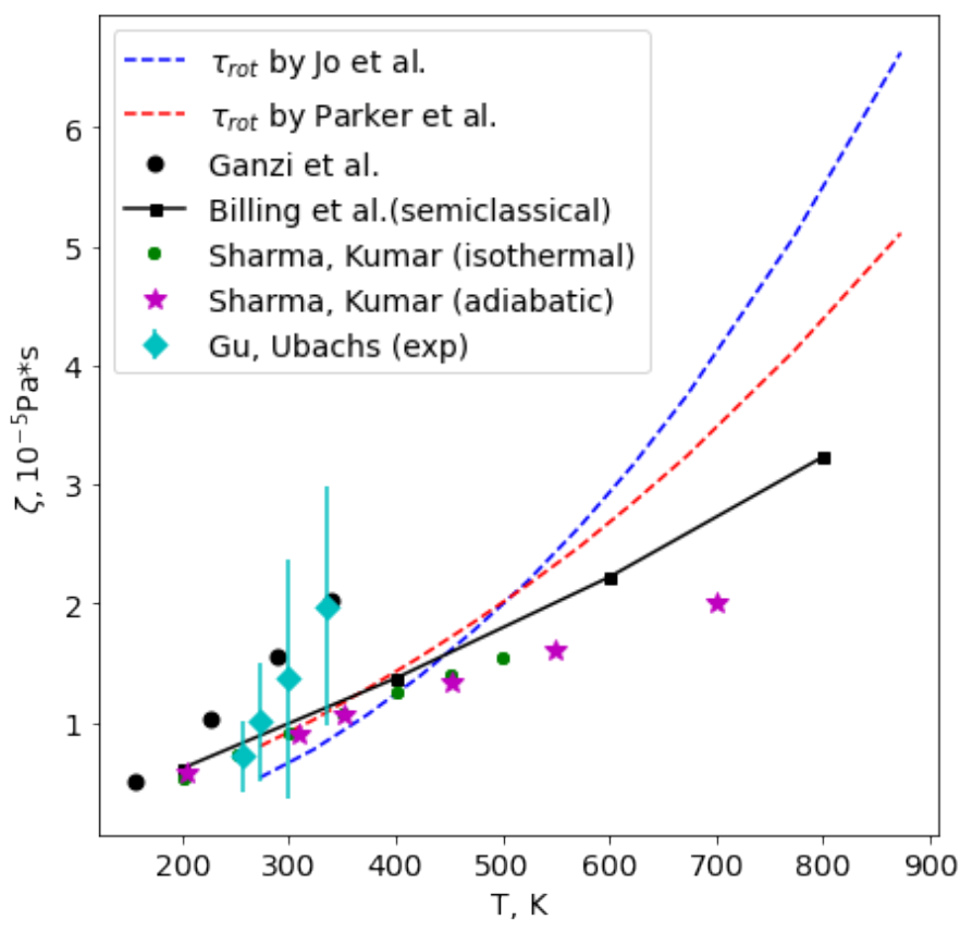
Let us assess first the bulk viscosity of diatomic species. In
Figure 1, we compare the bulk viscosity coefficient in nitrogen calculated using two models for the rotational relaxation time (the well-known model of Parker [
77] and the recent model proposed in [
78]) with experimental results of Ganzi and Sandler [
79] and Gu and Ubachs [
14,
15], molecular-dynamic simulations by Sharma et al [
49,
50], and semiclassical calculations by Billing and Wang [
80]. In experiments of [
79], the rotational collision numbers were found from thermal transpiration measurements; in [
14], spontaneous Rayleigh–Brillouin scattering was employed to evaluate the bulk viscosity coefficients. Molecular-dynamic simulations were carried out using either nonequilibrium [
49] or equilibrium [
50] approach; recent classical trajectory calculations of the rotational collision number are presented in [
81].
One can see that at low temperatures, all simulations are close to experimental measurements and the results fall within the error bar, although experimental results show a faster increase in
with
T. At
K, the overall agreement between various approaches is good, and the main source of uncertainty in our model is the rotational relaxation time since the contribution of vibrational modes is small. With the rising temperature, the difference between theoretical predictions of the bulk viscosity increases, which can be explained by uncertainties in both rotational and vibrational relaxation times. The model of [
78] yields a more sharp increase in
compared to the Parker theory [
77]; taking into account vibrational degrees of freedom leads to further growth of the bulk viscosity.
To evaluate the contributions of different degrees of freedom, let us estimate first the corresponding relaxation times. In
Figure 2, we compare
,
and the effective internal energy relaxation time
defined in Equation (
14) for N
, O
, CO
, CH
. Rotational relaxation times are calculated on the basis of the Parker theory [
77]; the vibrational relaxation time is calculated using the Millikan–White formula [
72]; for polyatomic molecules, the mode with the lowest frequency is used in this formula: bending mode for CO
and scissoring mode for CH
; for CO
, additional parameters adjustment was performed, to fit the experimental data of Simpson [
82] at low temperatures. Some experimental values of
are also plotted: data of Millikan [
72] for N
, O
, data of Lambert [
83] for CH
, and for CO
experimental results of Baganoff [
84], Itterbeek [
85], Eucken [
86]. For diatomic species and CO
, the calculated vibrational relaxation time is in close agreement with the experimental. For methane, the discrepancy is greater, especially with rising
T. This means that, according to Equation (
14), we may under-predict the vibrational energy contribution to the internal energy relaxation time and thus to the bulk viscosity. However, as is shown in
Section 6, using this vibrational relaxation time yields rather good agreement on the methane attenuation coefficient; therefore, we keep these values for our analysis.
As is seen in
Figure 2, at low temperatures the contribution of vibrational modes to the overall internal energy relaxation time
is low, and for diatomic species is hardly distinguishable at the logarithmic scale. With rising temperatures, the role of vibrational degrees of freedom becomes important, especially for polyatomic gases, where one can notice strong competition between rotational and vibrational modes at
K. Anyway, the effective relaxation time
is always found between
and
, and never attains large values comparable to
at low temperatures.
Now let us discuss the contribution of different internal degrees of freedom to the bulk viscosity in the framework of the one-temperature model. In the uncoupled phenomenological approach, it is commonly assumed [
41] that in diatomic gases at temperatures considerably lower than the characteristic vibrational temperature
, vibrational modes are frozen, and
. On the contrary, in polyatomic species with sufficiently fast vibrational relaxation, it is supposed in [
41] that
. For species considered in the present study, the characteristic vibrational temperatures are 3395 K for nitrogen and 2274 K for oxygen; in polyatomic species, the vibrational temperatures of the modes with the lowest frequency are 960 K for CO
and 1870 K for CH
. Thus, one can expect that at
K the bulk viscosity of N
and O
includes only the contribution of the rotational degrees of freedom. However, this is not exactly the case, as is seen from
Figure 3, where we plot the ratio of bulk and shear viscosity coefficients,
, as well as the ratio
. One can notice that in our coupled approach, the contribution of vibrational degrees of freedom to
is not negligible already at
K for oxygen and at
K for nitrogen; including vibrational modes causes an increase in
by 2-3 times. The reason is that the vibrational specific heat
starts increasing gradually at such temperatures, and at
T about 1000 K is comparable to
. Although for N
and O
at
K, the overall contribution of vibrational modes is not negligible since
.
For polyatomic species with several vibrational modes, the situation is quite different. The vibrational relaxation time is less than in N
and O
and gives a significant contribution to both
and
in the entire temperature range. Moreover, the vibrational specific heat is considerably greater in gases with multiple vibrational degrees of freedom. For the coupled model (
15), at low temperatures
and
are of the same order, but with rising temperature, the ratio
grows up to 20. It is worth mentioning that, contrarily to the uncoupled model [
41], the ratio of bulk and shear viscosity coefficients does not reach several thousand, as reported in [
41] for CO
at low temperatures. The latter result is the consequence of unjustified splitting of the bulk viscosity coefficient into the rotational and vibrational parts, see Equations (
16) and (
17). Since
in Equation (
17) is proportional to
, the overall bulk viscosity coefficient is greatly overestimated. In order to support this conclusion, we plot recent experimental results for CO
bulk viscosity [
16] (blue points in
Figure 3). One can see that our calculations are in good agreement with measurements of [
16].
Thus, we see that both in experiments and in the coupled kinetic-theory approach, the bulk viscosity coefficient is of the same order as that of shear viscosity. An interesting question, however, arises in this regard. It is known [
87] that in polyatomic gases, the attenuation coefficient
is considerably higher than in diatomic, and low values of bulk viscosity coefficient cannot reproduce such high values of
. This is why the idea of large bulk viscosity was supported in the fluid-dynamic community. In the next sections, we will show how to reproduce high values of attenuation coefficients in CO
and CH
without introducing artificially large bulk viscosity.
4. Two-Temperature Model
Under conditions of strong deviations from equilibrium, some microscopic processes may proceed at the gas-dynamic time scale. In single-component gases at moderate temperatures (except light gases), the slowest process is vibrational-translational (VT) relaxation. The kinetic scaling in this case can be written in the form
here,
,
are the characteristic times of vibrational-vibrational and vibrational-translational transitions. Note that in polyatomic gases with several vibrational modes, there are multiple channels of vibrational relaxation including intra- and inter-mode vibrational energy transitions. Characteristic times of these processes may differ by several orders of magnitude, which often requires introducing several vibrational temperatures. Multi-temperature models of CO
kinetics and transport processes based on the generalized Chapman–Enskog method were developed in [
23,
29,
88,
89,
90]. In the present study, we focus on the simplest two-temperature (2T) model, which does not distinguish different channels of vibrational relaxation in polyatomic gases but roughly captures main nonequilibrium effects.
Governing equations in the 2T model include Navier–Stokes–Fourier conservation equations coupled to the relaxation equation for the specific vibrational energy
:
The constitutive relations for the pressure tensor, heat flux, and vibrational energy flux in this case have the form
where
is the vibrational temperature,
is the relaxation (dynamic) pressure, and the transport coefficients are given by the expressions:
Strictly speaking,
-integrals in Equations (
9), (
10) and (
26) should be different since they are specified by the cross sections of rapid processes (see [
24]), which are different in the one-temperature and two-temperature models, see Equations (
3) and (
18). Nevertheless, the contribution of inelastic collisions to the
-integrals for the considered species is small [
24], and in the present study, only elastic collision cross sections are kept in the
-integrals.
The rate of vibrational energy relaxation is described using the Landau– Teller formulation:
The last expression is rather approximate for modeling the vibrational relaxation in polyatomic gases with multiple modes and inter-mode energy exchanges [
91], and we use it in the present study only for the sake of simplicity. In future work, we plan to consider advanced relaxation models proposed in [
89,
91], which take into account different temperatures of vibrational modes in polyatomic molecules.
An important feature of the two-temperature approach is that relaxation processes are modeled at various levels, depending on their characteristic times. Fast rotational relaxation is described in terms of the rotational bulk viscosity and heat conductivity depending on the temperature of local equilibrium degrees of freedom. Slow vibrational relaxation is governed by a separate equation, Equation (
22). The bulk viscosity in this case does not include contributions of the vibrational degrees of freedom and is fully specified by the rotational relaxation time.
Thus, assuming constant specific heats,
;
for linear molecules and
for nonlinear, we can simplify the expression for the bulk viscosity. For linear molecules we obtain:
and for nonlinear:
It is worth mentioning that the definition of bulk viscosity in the frame of the two-temperature model has some limitations in the case of polyatomic gases with several vibrational modes. The problem is that in the kinetic scaling (
18), all inter-mode VV exchanges are assumed to be fast, which is necessary for introducing a single vibrational temperature for different modes. Moreover, in order to correctly define the vibrational temperature, one has to assume that inter-mode transitions are resonant, which is a rough approximation, see [
29]. The problem can be overcome if a more rigorous multi-temperature approach is used, with a distinct vibrational temperature assigned to each mode.
5. Dispersion Relations in a Single-Component Gas
In this section, we derive the dispersion equations for the two-temperature and one-temperature models. Consider an acoustic wave propagating in a gas with the wave number
and frequency
. All gas parameters are expressed as sums of non-perturbed values
and small perturbations with amplitudes
:
Substituting them to the two-temperature governing Equations (
19)–(
22) and linearizing in the vicinity of the equilibrium state one obtains equations for dimensionless amplitudes
,
,
,
:
Here, is the thermal velocity, , are dimensionless coefficients of shear and bulk viscosity ( is the shear viscosity coefficient of the unperturbed flow), , ; and are dimensionless thermal conductivity coefficients and specific heats of translational-rotational and vibrational degrees of freedom, respectively, is the dimensionless frequency, is the pressure of the unperturbed flow.
This is a homogeneous system of linear equations. To find its non-trivial solution, we set to zero the system determinant and, therefore, solve the dispersion relation
The dispersion relation in the two-temperature approach represents a 6th-order nonlinear equation with respect to the wave number
k. Solving the dispersion equation one can find the phase velocity
and attenuation coefficient
It is also useful to introduce the non-dimensional attenuation coefficient per wavelength,
, which is used for the comparison with the experimental data:
In order to derive the dispersion equation in the one-temperature approach, a similar procedure is applied to a set of governing Equations (
4)–(
6). The dispersion relation in this case is a 4th-order nonlinear equation with respect to
k:
Here,
is the total dimensionless thermal conductivity coefficient including both translational and internal contributions. Note that the bulk viscosity coefficient in dispersion relations (
39) and (
42) are different: in the first case, it is specified by Equation (
27), and in the latter case—by Equation (
15).
Asymptotic methods may be used in the dispersion relations in order to obtain simplified expressions as discussed for instance in [
92]. Thus, the Stokes–Kirchhoff relation (
2) can be derived from the one-temperature dispersion equation (
42). Moreover, these asymptotic methods could be used to obtain analytical expressions of the attenuation coefficients for acoustic modes in the presence of vibrational relaxation.
6. Attenuation Coefficient in a Single-Component Gas
Let us compare the attenuation coefficient calculated using different models with that measured experimentally in [
87,
93]. We assess the two-temperature and one-temperature approaches and the Stokes–Kirchhoff equation with various data for the transport coefficients. For carbon dioxide, we use the transport model developed in our previous work [
23] (marked “Our model” in the figures) as well as the data for the shear viscosity and total thermal conductivity reported in NIST [
94] and calculated using the Cantera package [
95]. For other species, we use the data provided by [
94,
95]. Note that in these latter sources, the one-temperature model is implemented, and in order to separate the contributions of different internal modes to the thermal conductivity, we use the Eucken formula [
96] generalized in [
97] for the case of the two-temperature model.
The dispersion equations were solved numerically using the high-precision mpmath Python library, version 1.2.1. The solutions were sought in the vicinity of the points having physical meaning; unphysical solutions were disregarded.
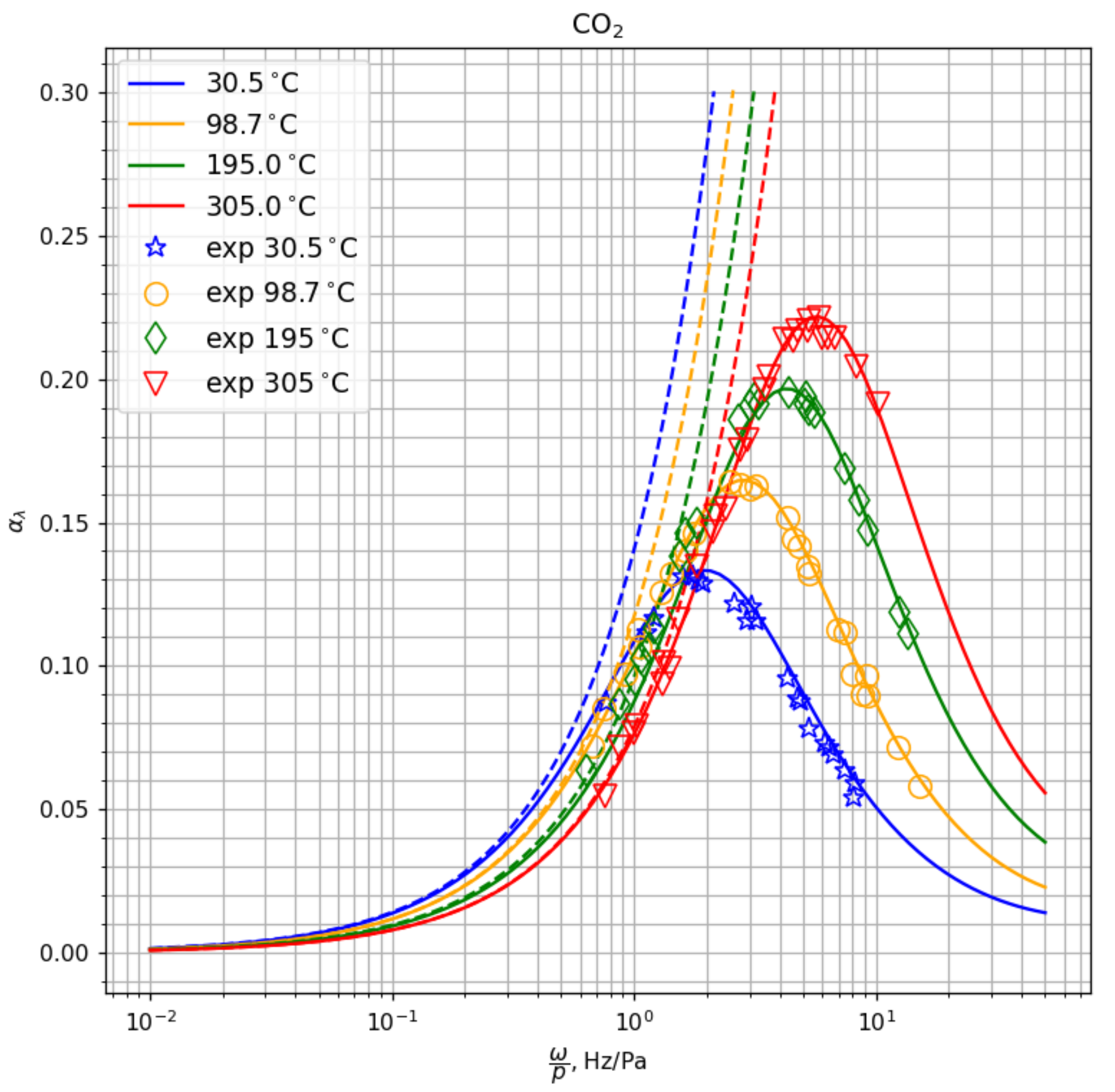
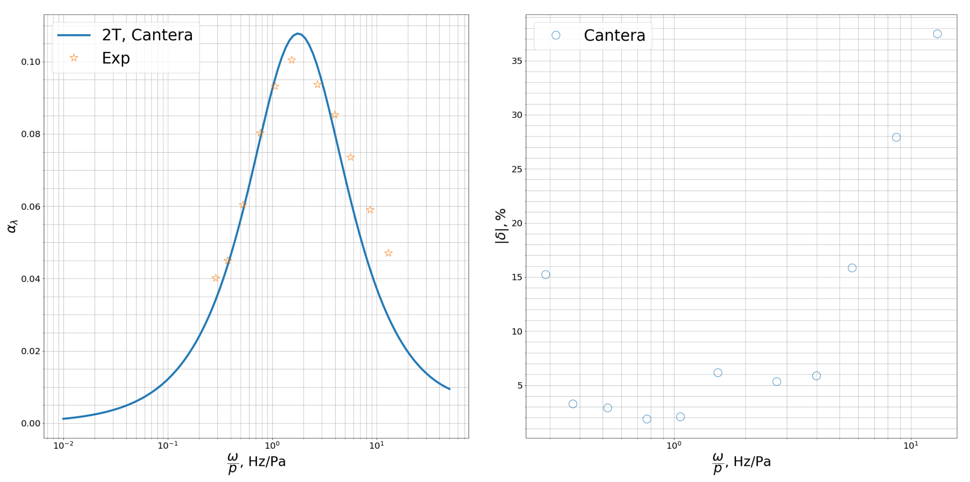
In
Figure 4,
Figure 5 and
Figure 6 we present the dimensionless attenuation coefficient per wavelength
as a function of frequency related to pressure,
, for CO
, CH
, O
. For polyatomic species, we also give the deviation of the coefficients obtained using the two-temperature model from the experimental data,
in %. One can see that the model of transport coefficients weakly affects the attenuation coefficient. On the other hand, the choice of the relaxation model (weak nonequilibrium, 1T, or strong nonequilibrium, 2T) is crucial for the correct prediction of the attenuation coefficient. For polyatomic species, the two-temperature model provides excellent agreement with the measured attenuation coefficient in the wide frequency range (except for very high frequencies in methane,
Hz/Pa where we see some deviations). The location and the value of the maximum in
is well predicted by the two-temperature model whereas the one-temperature model shows monotonic behavior of the attenuation coefficient.
For oxygen, the contribution of relaxation to the attenuation coefficient is weak, and the classical Stokes–Kirchhoff formula yields satisfactory agreement with the experimental data which do not show any peaks in
. The same conclusion is drawn in [
87]. We do not plot the deviation from the experimental data for this case since the attenuation coefficient is rather small in the considered frequency range, and therefore the uncertainty may be high.
In the results presented in
Figure 4 and
Figure 5, the bulk viscosity in the one-temperature approach is calculated according to our coupled model (
15) without separating rotational and vibrational modes. As we see, low bulk viscosity coefficients obtained in this case cannot reproduce high values of the attenuation coefficient and its maximum. We have carried out an additional numerical experiment using in the dispersion relation the data of Cramer [
41] for the bulk viscosity of CO
, which yields the ratio
. The results are presented in
Figure 7 for several temperatures. Solid lines correspond to 2T calculations, dashed lines—to the 1T model with large
, symbols—to the experiment [
93]. One can see that high values of bulk viscosity considerably improve predicted values of
at low frequencies (
Hz/Pa). With rising frequency, the attenuation coefficient increases indefinitely, and the 1T model does not predict the maximum in
. This is clear since in the frame of linear theory, the Stokes–Kirchhoff formula provides a linear dependency of
on the frequency. Therefore, using the large bulk viscosity does not help to overcome the problem of the discrepancy in the attenuation coefficient calculated using the 1T model in the wide frequency range.
This result is not surprising. In the sound propagation problem, when the gas pressure is high, the NSF equation can be derived from the gas kinetic equation only when the product of sound frequency and mean relaxation time is small; when the vibrational relaxation time is large, the one-temperature NSF equation certainly will lose accuracy with rising frequency. In this case, other approaches have to be used.
It is worth mentioning that the theory developed in the frame of the rational extended thermodynamics (RET) [
34] also provides good agreement with the experimental data on the attenuation coefficient and predicts very well the first maximum location and its height. Moreover, the two-temperature model proposed in the present study can be treated as a particular case of the more general RET theory. However, in the RET simulations, the relaxation time and the bulk viscosity coefficient are the model parameters that are used to fit the experimental data. In our case, both the relaxation time and all transport coefficients can be calculated self-consistently in the frame of the Chapman–Enskog formalism and are not to be adjusted for better agreement with experiments.
7. Dispersion Relation in a Mixture with Slow Vibrational Relaxation
This section is devoted to the generalization of the two-temperature model for the case of gas mixtures with strongly nonequilibrium vibrational relaxation in the absence of chemical reactions. We derive the corresponding dispersion equation and discuss the preliminary results for binary and five-component mixtures. Wave propagation in gas mixtures with vibrational relaxation was considered previously in [
98,
99,
100,
101]. The theory developed in [
98,
99,
100] was developed on the basis of the Euler equations, and therefore the effects of relaxation and viscosity were studied separately; diffusion processes were neglected. In [
101], the state-to-state model was considered for a few vibrational states of diatomic molecules, and all dissipative processes including diffusion and thermal diffusion were taken into account. In the present study, we derive the multi-temperature dispersion equation in a fully coupled approach, accounting for viscosity, bulk viscosity, thermal conductivity, diffusion, thermal diffusion, and vibrational relaxation.
The fluid-dynamic variables providing the closed description of a gas mixture flow with slow vibrational relaxation include number densities of chemical species
c,
, velocity
, temperature
, and vibrational temperature of species
c,
. The governing equations for this set of variables were derived in [
24]:
here,
,
,
,
are density, diffusion velocity, specific vibrational energy, and vibrational energy flux for species
c,
L is the number of species. The total specific energy of the mixture
E is defined as
The pressure tensor has a form similar to the case of a single-component gas, see Equation (
23). However, the transport coefficients are calculated differently; they cannot be written analytically but are obtained as solutions of linear transport systems (see [
19,
21,
24]). In the general case, they cannot be expressed explicitly in terms of species transport coefficients. Nevertheless, for approximate evaluations, mixing rules can be applied, such as the Wilke’s formula for the shear viscosity [
102] and the formulas proposed in [
21,
103] for thermal conductivity, bulk viscosity, and other transport coefficients.
The diffusion velocity
is determined by diffusion and thermal diffusion processes with corresponding multi-component diffusion and thermal diffusion coefficients
and
:
here
is the diffusive driving force
The total heat flux
depends on the gradients of temperature
T, vibrational temperature
and includes the terms associated with diffusion and thermal diffusion:
is the partial thermal conductivity coefficient of translational and rotational degrees of freedom,
is the vibrational thermal conductivity coefficient for species
c. The flux of vibrational energy
depends on the gradient of
,
The rate of vibrational energy relaxation
is calculated using the Landau–Teller model applied to the vibrational energy of each species
c
where
is the vibrational relaxation time which, strictly speaking, depends not only on the species
c but also on the collision partner.
Let us derive the dispersion relation. We express again the gas parameters as a sum of non-perturbed values
,
,
,
,
and small perturbations with amplitudes
, wave number
and frequency
:
Substituting these parameters into the governing equations, keeping only linear terms and taking into account normalizing conditions for the diffusion and thermal diffusion coefficients [
24]
after lengthy calculations, we obtain the linear system
Here, as before,
are dimensionless transport coefficients (
is the shear viscosity of the unperturbed gas mixture);
and
are dimensionless specific heats for species
c,
and
m are the mass of
c species and the average mass of the mixture,
are the Schmidt numbers corresponding to the multicomponent diffusion and thermal diffusion coefficients. Note that, for the sake of convenience, one of the equations for species number densities
is replaced with the continuity equation.
In order to find a non-trivial solution of the linear system (
59)–(
63), we set to zero its determinant,
(
is the matrix of the system) and thus obtain the dispersion equation which is solved with respect to the wave number
k. The phase velocity and attenuation coefficients are then found using Equation (
40).
The dispersion relation derived in this way is the most general since it is determined by the full set of equations for a nonequilibrium mixture flow and includes self-consistently all possible dispersion mechanisms: viscosity, thermal conductivity, bulk viscosity, diffusion, thermal diffusion, and vibrational relaxation. Contributions of various dissipative processes are not separated into independent terms, and no simplifications are introduced except linearization of the original system for small perturbations. The price for such generality is the order of the resulting complex equation: for instance, for a five-component mixture we obtain a 26th-order equation which is rather difficult to solve numerically.
The derived dispersion equation is first solved for a binary mixture CO
–N
. The attenuation coefficient is presented in
Figure 8 and compared with the experimental data [
87]. One can see satisfactory agreement with experimental values; the location of the maximum is predicted correctly as well as its height. The discrepancy, however, increases with frequency.
Next, the dispersion relation was assessed for five-component mixtures containing hydrocarbons. For such mixtures, the full problem becomes too much complicated, especially if we include considerable fractions of heavy hydrocarbons. In particular, at high frequencies, we meet numerical problems with the convergence of the solution; the attenuation coefficient sometimes drops sharply at
Hz/Pa. Since we have no experimental evidence of such behavior (no experimental data on multi-component mixtures were found in the literature), we decided to keep only the results for light hydrocarbons. Two mixture compositions were considered: (1) N
(2%)–CH
(91%)–CO
(1%)–C
H
(3%)–C
H
(3%) and (2) N
(14%)–CH
(47%)–CO
(2%)–C
H
(22%)–C
H
(15%). The results are presented in
Figure 9 for two temperatures.
Let us assess the contribution of diffusion processes to the attenuation coefficient. In the absence of diffusion and thermal diffusion, all Schmidt numbers in Equations (
59)–(
63) can be set to zero, and we obtain a simplified linear system
The order of the resulting dispersion equation based on this system is considerably lower, and the solution is stable and converging.
The results obtained disregarding the diffusion processes are plotted in
Figure 9 using dashed lines. It is seen that the role of diffusion is negligible in the low and moderate frequency range. For high frequencies, the source of discrepancy is not completely clear: we assume that it could the error of solving the high-order complex equation rather than the contribution of diffusion and thermal diffusion. This issue requires further investigation and will be considered in our future studies.
8. Conclusions
Two different continuum flow descriptions in the framework of the generalized Chapman–Enskog method are discussed: the one-temperature model for weak deviations from equilibrium and the multi-temperature model suitable for strong nonequilibrium flows with slow VT relaxation. In the first approach, all relaxation processes are modeled by including bulk viscosity and internal thermal conductivity to the stress tensor and heat flux. In the latter approach, fast relaxation processes are taken into account by means of rotational bulk viscosity whereas slow VT processes are described by an additional relaxation equation coupled to the fluid-dynamic equations. Governing equations and constitutive relations for both models are written in the first-order approximation of the Chapman–Enskog method corresponding to the viscous gas flows (NSF approach), and the dispersion equations are derived in a fully consistent way, without separation of various mechanisms of sound wave attenuation. In the most general case of vibrationally nonequilibrium multi-component gas mixture, these mechanisms include viscosity, thermal conductivity, bulk viscosity, diffusion, thermal diffusion, and vibrational relaxation. Since we do not introduce any additional simplifications, the proposed dispersion relations involve coupled sound absorption mechanisms, and therefore are more general than commonly used relations based on the separation of classical Stokes–Kirchhoff attenuation and relaxation. Such an approach allows accurate evaluation of different contributions to the attenuation coefficients of polyatomic gases and their mixtures; this will be the objective of our further studies.
The contributions of rotational and vibrational modes to the bulk viscosity coefficient are considered in detail. It is proved that in the one-temperature approach, the bulk viscosity of polyatomic gases is greatly overestimated when rotational and vibrational contributions are split into independent terms. On the contrary, using the effective internal energy relaxation time yields good agreement with experimental data and molecular-dynamic simulations. Complete disregarding of the vibrational contribution leads to noticeable inaccuracy in the bulk viscosity coefficient even in diatomic species at temperatures much lower than the characteristic vibrational temperature. In the multi-temperature approach, the bulk viscosity does not include contributions of vibrational modes, which are rather taken into account by means of separate relaxation equations.
Attenuation coefficients were calculated for diatomic and polyatomic species using various models. In oxygen, the main contribution to the wave attenuation is given by the classical Stokes–Kirchhoff mechanism and the role of relaxation is weak. In polyatomic species, the developed two-temperature model provides excellent agreement with the experimental attenuation coefficient and correctly reproduces both the location and the value of its maximum. Neither one-temperature dispersion relations nor the Stokes–Kirchhoff formula reproduces the non-monotonic behavior of the attenuation coefficient. Large bulk viscosity coefficients reported in some previous studies may improve in some way the accuracy of at low frequencies but still fail to describe it at moderate and high frequencies. The model for other transport coefficients (shear viscosity and heat conductivity) weakly affects the attenuation coefficient since the main contribution comes from slow vibrational relaxation processes. For multi-component mixtures, the role of diffusion and thermal diffusion is found to be negligible at low and moderate frequencies, which considerably simplifies solving the dispersion equation.
The proposed approach, however, has some limitations since it is based on the multi-temperature model which does not capture deviations from the Boltzmann distributions. Theoretically, it can be easily generalized for the state-to-state model, but the resulting dispersion equations will be of a very high order. Rational extended thermodynamics also may provide a tool to go beyond this continuum approach.
It should be noted that recent publications reporting high values of bulk viscosity have resulted in many CFD studies searching for new physical effects in compressible flows. We have to admit that implementing high bulk viscosity in the one-temperature NSF equations is a misuse that may lead to unphysical results. On the other hand, introducing correct values of bulk viscosity in shock wave studies (and other flows with high gradients) may considerably improve the solution.
Finally, we would like to emphasize that in the continuum approach, it is of great importance to correctly establish the kinetic scaling and develop the flow model according to this scaling. Continuum models developed for a certain kinetic scaling generally fail to describe the flows which are farther from the equilibrium; the remedy is in developing more detailed models taking into account a greater number of slow relaxation processes. In such a way, the limits of the continuum approach can be considerably extended.


