
Assessment of a RANS Transition Model with Flapping Foils at Moderate Reynolds Numbers

Abstract
:1. Introduction
2. Simulation Setup
2.1. Kinematic Framework
2.2. Numerical Framework
3. Results
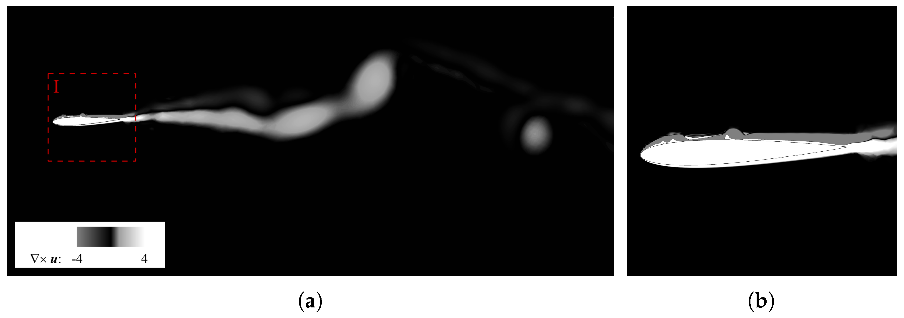
3.1. NACA0012
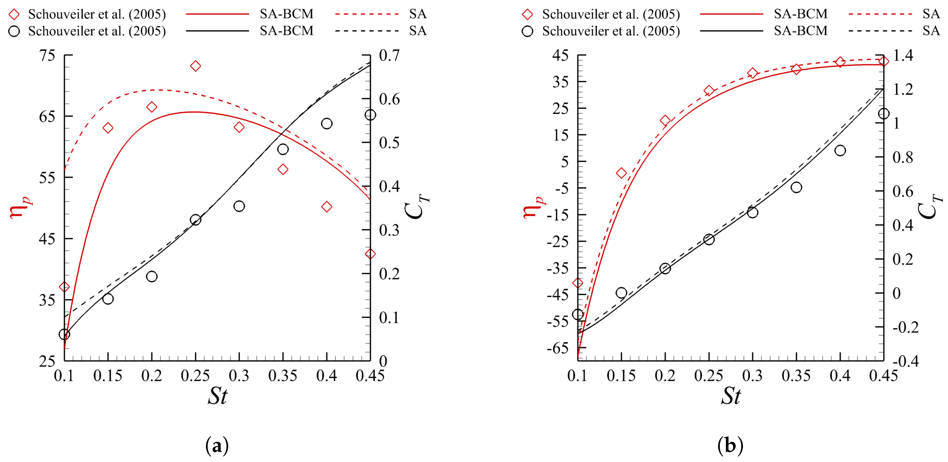
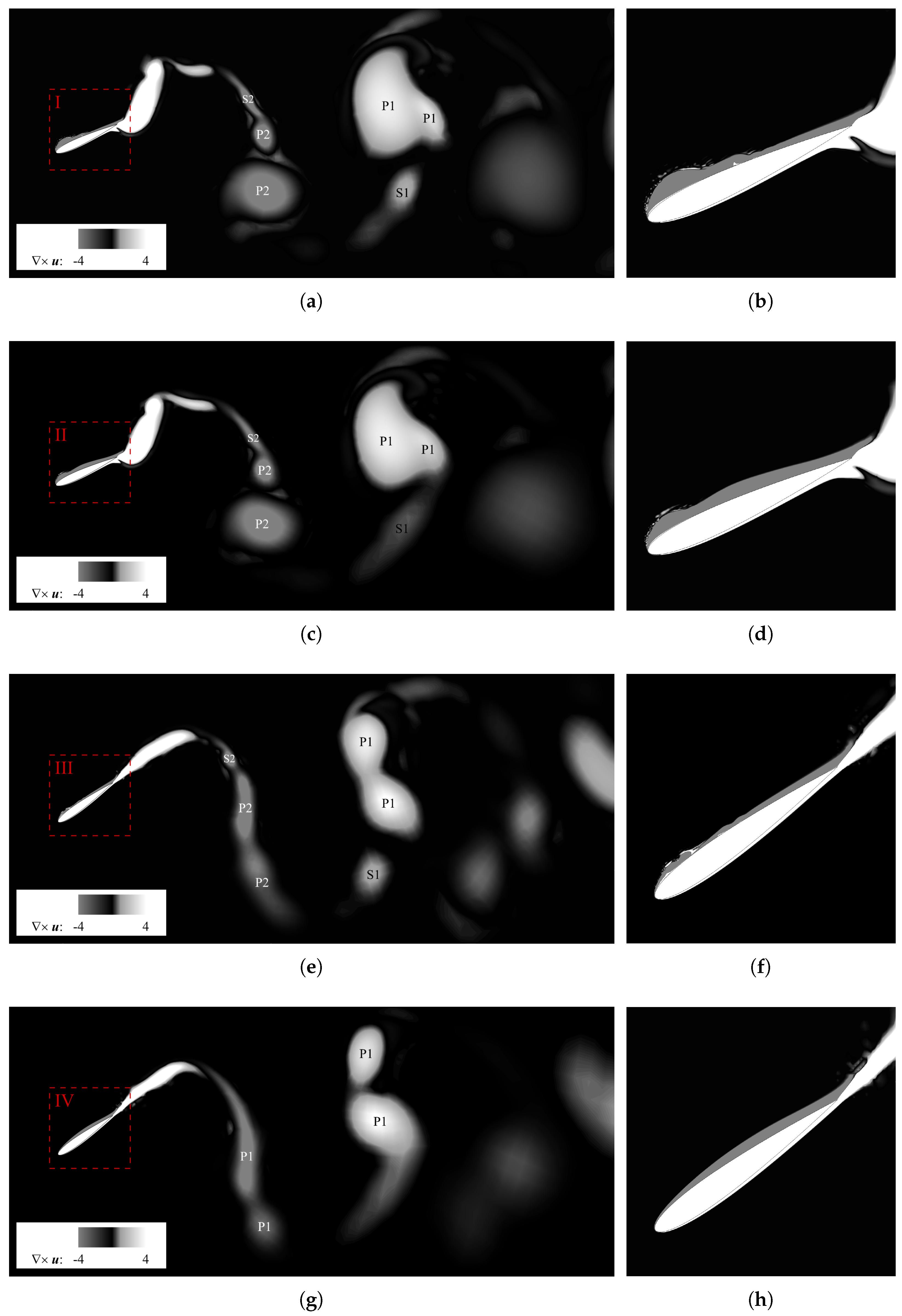
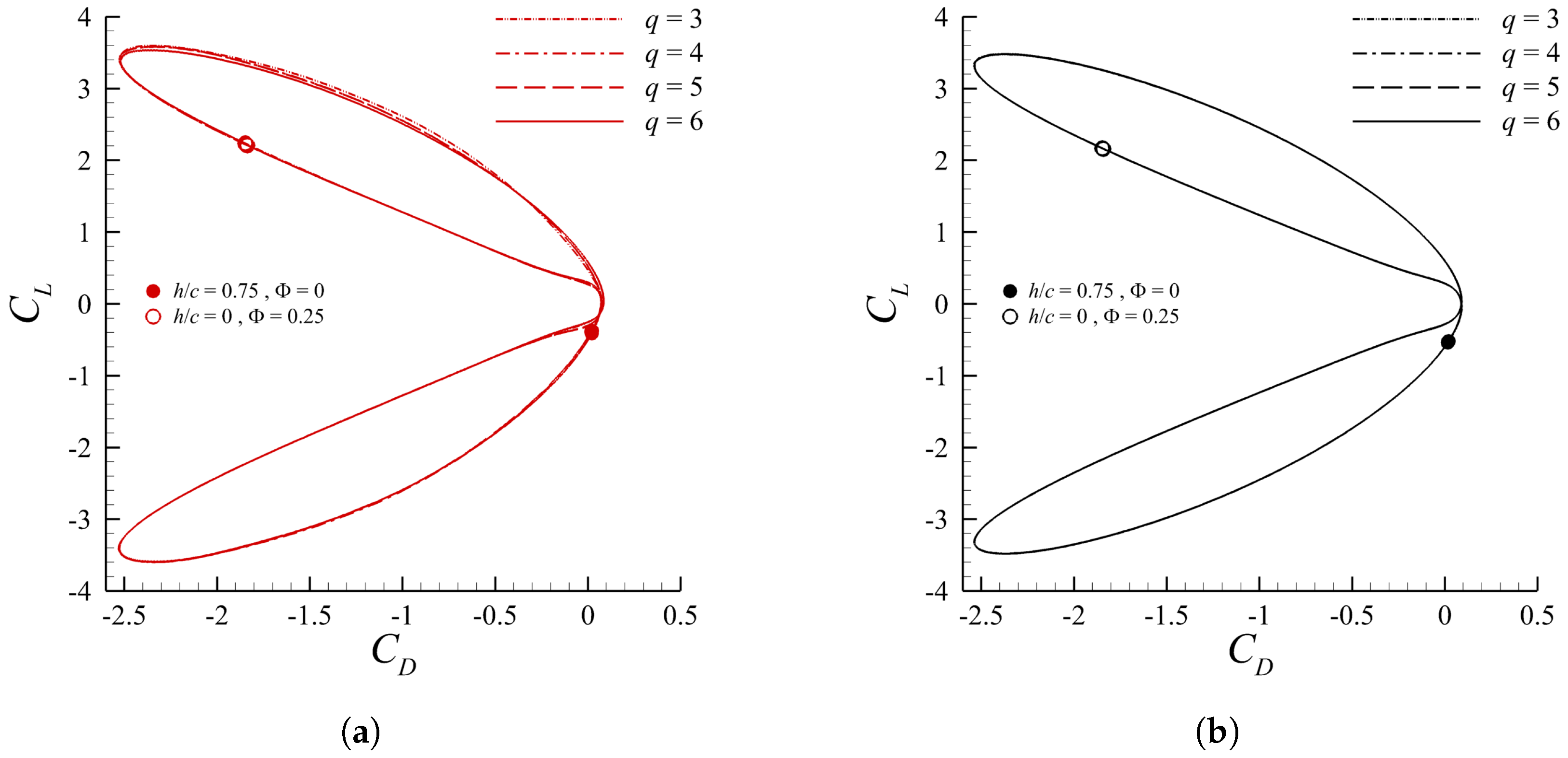
3.2. SD7003
3.2.1. Case 1
3.2.2. Case 2
4. Conclusions
Supplementary Materials
Author Contributions
Funding
Data Availability Statement
Conflicts of Interest
Abbreviations
| DG | Discontinuous Galerkin |
| DNS | Direct numerical simulation |
| DOF | Degrees of freedom |
| GMRES | Generalized minimal residual method |
| ILES | Implicit large eddy simulation |
| LES | Large eddy simulation |
| LEV | Leading-edge vortex |
| PDE | Partial differential equation |
| PIV | Particle image velocimetry |
| RANS | Reynolds-averaged Navier–Stokes |
| SA | Spalart–Allmaras |
| SA-BCM | Spalart–Allmaras—Bas-Cakmakcioglu-Mura |
| TEV | Trailing-edge vortex |
References
- Knoller, A. Die gesetzedes luftwiderstandes. Flug Und Mot. 1909, 3, 1–7. [Google Scholar]
- Betz, A. Ein beitrag zur erklaerung segelfluges. Z. Flugtech Mot. 1912, 3, 269–272. [Google Scholar]
- Von Kármán, T.; Burgers, J. General Aerodynamic Theory-Perfect Fluids. Aerodyn. Theory 1943, 2, 346–349. [Google Scholar]
- Lighthill, S.J. Mathematical Biofluiddynamics; Society for Industrial and Applied Mathematics: Philadelphia, PA, USA, 1975. [Google Scholar] [CrossRef]
- Wu, X.; Zhang, X.; Tian, X.; Li, X.; Lu, W. A review on fluid dynamics of flapping foils. Ocean. Eng. 2020, 195, 106712. [Google Scholar] [CrossRef]
- Triantafyllou, M.; Triantafyllou, G.; Gopalkrishnan, R. Wake mechanics for thrust generation in oscillating foils. Phys. Fluids Fluid Dyn. 1991, 3, 2835–2837. [Google Scholar] [CrossRef]
- Read, D.; Hover, F.; Triantafyllou, M. Forces on oscillating foils for propulsion and maneuvering. J. Fluids Struct. 2003, 17, 163–183. [Google Scholar] [CrossRef]
- Schouveiler, L.; Hover, F.; Triantafyllou, M. Performance of flapping foil propulsion. J. Fluids Struct. 2005, 20, 949–959. [Google Scholar] [CrossRef]
- Anderson, J.M.; Streitlien, K.; Barrett, D.; Triantafyllou, M.S. Oscillating foils of high propulsive efficiency. J. Fluid Mech. 1998, 360, 41–72. [Google Scholar] [CrossRef] [Green Version]
- Ol, M.V.; Reeder, M.; Fredberg, D.; McGowan, G.Z.; Gopalarathnam, A.; Edwards, J.R. Computation vs. Experiment for High-Frequency Low-Reynolds Number Airfoil Plunge. Int. J. Micro Air Veh. 2009, 1, 99–119. [Google Scholar] [CrossRef]
- Visbal, M. High-fidelity simulation of transitional flows past a plunging airfoil. AIAA J. 2009, 47, 2685–2697. [Google Scholar] [CrossRef]
- Krais, N.; Schnücke, G.; Bolemann, T.; Gassner, G.J. Split form ALE discontinuous Galerkin methods with applications to under-resolved turbulent low-Mach number flows. J. Comput. Phys. 2020, 421, 109726. [Google Scholar] [CrossRef]
- Fröhlich, J.; Von Terzi, D. Hybrid LES/RANS methods for the simulation of turbulent flows. Prog. Aerosp. Sci. 2008, 44, 349–377. [Google Scholar] [CrossRef]
- Chaouat, B. The state of the art of hybrid RANS/LES modeling for the simulation of turbulent flows. Flow Turbul. Combust. 2017, 99, 279–327. [Google Scholar] [CrossRef] [Green Version]
- Yang, W.; Fan, Z.; Deng, X.; Zhao, X. RANS/LES Simulation of Low-Frequency Flow Oscillations on a NACA0012 Airfoil Near Stall. In Proceedings of the 2021 International Symposium on Electrical, Electronics and Information Engineering, Seoul, Republic of Korea, 19–21 February 2021; pp. 62–65. [Google Scholar]
- Sanchez-Rocha, M.; Kirtas, M.; Menon, S. Zonal hybrid RANS-LES method for static and oscillating airfoils and wings. In Proceedings of the 44th AIAA Aerospace Sciences Meeting and Exhibit, Reno, Nevada, 9–12 January 2006; p. 1256. [Google Scholar]
- Menter, F.R.; Langtry, R.B.; Likki, S.R.; Suzen, Y.B.; Huang, P.G.; Völker, S. A Correlation-Based Transition Model Using Local Variables—Part I: Model Formulation. J. Turbomach. 2004, 128, 413–422. [Google Scholar] [CrossRef]
- Langtry, R.B.; Menter, F.R.; Likki, S.R.; Suzen, Y.B.; Huang, P.G.; Völker, S. A Correlation-Based Transition Model Using Local Variables—Part II: Test Cases and Industrial Applications. J. Turbomach. 2004, 128, 423–434. [Google Scholar] [CrossRef]
- Walters, D.K.; Leylek, J.H. A New Model for Boundary Layer Transition Using a Single-Point RANS Approach. J. Turbomach. 2004, 126, 193–202. [Google Scholar] [CrossRef]
- Carreño Ruiz, M.; D’Ambrosio, D. Validation of the γ-Reθ Transition Model for Airfoils Operating in the Very Low Reynolds Number Regime. Flow Turbul. Combust. 2022, 109, 279–308. [Google Scholar] [CrossRef]
- Ashraf, M.; Young, J.; Lai, J. Oscillation frequency and amplitude effects on plunging airfoil propulsion and flow periodicity. AIAA J. 2012, 50, 2308–2324. [Google Scholar] [CrossRef]
- Li, X.; Liu, Y.; Kou, J.; Zhang, W. Reduced-order thrust modeling for an efficiently flapping airfoil using system identification method. J. Fluids Struct. 2017, 69, 137–153. [Google Scholar] [CrossRef]
- Young, J.; Lai, J.C. Oscillation frequency and amplitude effects on the wake of a plunging airfoil. AIAA J. 2004, 42, 2042–2052. [Google Scholar] [CrossRef]
- Wang, Z.; Du, L.; Zhao, J.; Sun, X. Structural response and energy extraction of a fully passive flapping foil. J. Fluids Struct. 2017, 72, 96–113. [Google Scholar] [CrossRef]
- Cakmakcioglu, S.; Bas, O.; Mura, R.; Kaynak, U. A Revised One-Equation Transitional Model for External Aerodynamics. In Proceedings of the AIAA Aviation 2020 Forum, Virtual Event, 15–19 June 2020. [Google Scholar] [CrossRef]
- Cakmakcioglu, S.C.; Bas, O.; Kaynak, U. A correlation-based algebraic transition model. Proc. Inst. Mech. Eng. Part J. Mech. Eng. Sci. 2017, 232, 3915–3929. [Google Scholar] [CrossRef]
- Mura, R.; Cakmakcioglu, S.C. A Revised One-Equation Transitional Model for External Aerodynamics—Part I: Theory, Validation and Base Cases. In Proceedings of the AIAA Aviation 2020 Forum, Virtual Event, 15–19 June 2020. [Google Scholar] [CrossRef]
- Bassi, F.; Crivellini, A.; Rebay, S.; Savini, M. Discontinuous Galerkin solution of the Reynolds averaged Navier-Stokes and k-ω turbulence model equations. Comput. Fluids 2005, 34, 507–540. [Google Scholar] [CrossRef]
- Bassi, F.; Crivellini, A.; Di Pietro, D.; Rebay, S. An implicit high-order discontinuous Galerkin method for steady and unsteady incompressible flows. Comput. Fluids 2007, 36, 1529–1546. [Google Scholar] [CrossRef]
- Crivellini, A.; D’Alessandro, V.; Bassi, F. A Spalart-Allmaras turbulence model implementation in a discontinuous Galerkin solver for incompressible flows. J. Comput. Phys. 2013, 241, 388–415. [Google Scholar] [CrossRef]
- Crivellini, A.; D’Alessandro, V.; Bassi, F. High-order discontinuous Galerkin solutions of three-dimensional incompressible RANS equations. Comput. Fluids 2013, 81, 122–133. [Google Scholar] [CrossRef]
- Gledhill, I.M.A.; Roohani, H.; Forsberg, K.; Eliasson, P.; Skews, B.W.; Nordström, J. Theoretical treatment of fluid flow for accelerating bodies. Theor. Comput. Fluid Dyn. 2016, 30, 449–467. [Google Scholar] [CrossRef] [Green Version]
- Bassi, F.; Botti, L.; Colombo, A.; Crivellini, A.; Franchina, N.; Ghidoni, A. Assessment of a high-order accurate Discontinuous Galerkin method for turbomachinery flows. Int. J. Comput. Fluid Dyn. 2016, 30, 307–328. [Google Scholar] [CrossRef]
- Spalart, P.; Allmaras, S. A one-equation turbulence model for aerodynamic flows. In Proceedings of the 30th Aerospace Sciences Meeting and Exhibit, Reno, NV, USA, 6–9 January 1992. [Google Scholar] [CrossRef]
- Menter, F.R.; Matyushenko, A.; Lechner, R.; Stabnikov, A.; Garbaruk, A. An Algebraic LCTM Model for Laminar–Turbulent Transition Prediction. Flow Turbul. Combust. 2022, 109, 841–869. [Google Scholar] [CrossRef]
- Bassi, F.; Crivellini, A.; Di Pietro, D.A.; Rebay, S. An artificial compressibility flux for the discontinuous Galerkin solution of the incompressible Navier-Stokes equations. J. Comput. Phys. 2006, 218, 794–815. [Google Scholar] [CrossRef]
- Lang, J.; Verwer, J. ROS3P—An accurate third-order Rosenbrock solver designed for parabolic problems. BIT 2001, 41, 731–738. [Google Scholar] [CrossRef]
- Rumsey, C.L. Apparent transition behavior of widely-used turbulence models. Int. J. Heat Fluid Flow 2007, 28, 1460–1471. [Google Scholar] [CrossRef] [Green Version]
- Franciolini, M.; Botti, L.; Colombo, A.; Crivellini, A. p-Multigrid matrix-free discontinuous Galerkin solution strategies for the under-resolved simulation of incompressible turbulent flows. Comput. Fluids 2020, 206, 104558. [Google Scholar] [CrossRef]
- Geuzaine, C.; Remacle, J.F. Gmsh: A 3-D finite element mesh generator with built-in pre-and post-processing facilities. Int. J. Numer. Methods Eng. 2009, 79, 1309–1331. [Google Scholar] [CrossRef]
- Williamson, C.H.; Roshko, A. Vortex formation in the wake of an oscillating cylinder. J. Fluids Struct. 1988, 2, 355–381. [Google Scholar] [CrossRef]
- Koochesfahani, M.M. Vortical patterns in the wake of an oscillating airfoil. AIAA J. 1989, 27, 1200–1205. [Google Scholar] [CrossRef]
- Ol, M. Vortical structures in high frequency pitch and plunge at low Reynolds number. In Proceedings of the 37th AIAA Fluid Dynamics Conference and Exhibit, Miami, FL, USA, 25–28 June 2007; p. 4233. [Google Scholar]
- Andersen, A.; Bohr, T.; Schnipper, T.; Walther, J.H. Wake structure and thrust generation of a flapping foil in two-dimensional flow. J. Fluid Mech. 2017, 812. [Google Scholar] [CrossRef] [Green Version]
- Cimarelli, A.; Franciolini, M.; Crivellini, A. On the kinematics and dynamics parameters governing the flow in oscillating foils. J. Fluids Struct. 2021, 101, 103220. [Google Scholar] [CrossRef]
- Guglielmini, L.; Blondeaux, P.; Vittori, G. A simple model of propulsive oscillating foils. Ocean. Eng. 2004, 31, 883–899. [Google Scholar] [CrossRef]


| SA | SA-BCM | Visbal [11] | Krais et al. [12] |
|---|---|---|---|
| −0.072 | −0.073 | −0.083 | −0.082 |
| q | SA | SA-BCM |
|---|---|---|
| 1 | 0.210 | 0.215 |
| 2 | 0.196 | 0.204 |
| 3 | 0.194 | 0.204 |
| 4 | 0.194 | 0.205 |
| 5 | 0.194 | 0.205 |
| 6 | 0.194 | 0.205 |
| Case | SA | SA-BCM | Visbal [11] |
|---|---|---|---|
| , | 0.193 | 0.205 | 0.225 |
| , | 0.158 | 0.133–0.148 | 0.133 |
Disclaimer/Publisher’s Note: The statements, opinions and data contained in all publications are solely those of the individual author(s) and contributor(s) and not of MDPI and/or the editor(s). MDPI and/or the editor(s) disclaim responsibility for any injury to people or property resulting from any ideas, methods, instructions or products referred to in the content. |
© 2023 by the authors. Licensee MDPI, Basel, Switzerland. This article is an open access article distributed under the terms and conditions of the Creative Commons Attribution (CC BY) license (https://creativecommons.org/licenses/by/4.0/).
Share and Cite
Alberti, L.; Carnevali, E.; Crivellini, A. Assessment of a RANS Transition Model with Flapping Foils at Moderate Reynolds Numbers. Fluids 2023, 8, 23. https://doi.org/10.3390/fluids8010023
Alberti L, Carnevali E, Crivellini A. Assessment of a RANS Transition Model with Flapping Foils at Moderate Reynolds Numbers. Fluids. 2023; 8(1):23. https://doi.org/10.3390/fluids8010023
Chicago/Turabian StyleAlberti, Luca, Emanuele Carnevali, and Andrea Crivellini. 2023. "Assessment of a RANS Transition Model with Flapping Foils at Moderate Reynolds Numbers" Fluids 8, no. 1: 23. https://doi.org/10.3390/fluids8010023