1. Introduction
Automotive aerodynamics is an area of particular interest to researchers due to the potential impact of drag reduction on fuel consumption and global emissions. The current political climate and emphasis on reducing human impact on the environment has shifted automotive perspective in recent times, with global emissions making up a key policy area for many governments worldwide. With the shift to reducing emissions globally, including the adoption of Battery Electric Vehicles highlighted in recent months with the COP26 summit in the UK—drag reduction is a key focus of the wider automotive industry.
Considering that vehicle shape is proprietary and varies significantly across the wider automotive market, studies utilising bluff bodies that mimic key geometric features adopted by market competitors is a necessity in order to study the fundamental physics and aerodynamics of each geometric feature. Various bodies such as the Ahmed Body [
1] and the Windsor Body [
2] have proven to be efficient methods used to test numerical and experimental techniques on representative and salient flow physiology with somewhat reduced geometric complexity. A extensive array of literature on these bodies has been generated, allowing authors and the industry to obtain greater insights into areas such as drag reduction, vehicle stability and noise, vibration and harshness. Furthermore, these geometries have also presented an opportunity for the industry and academia to validate computational methodologies.
Whilst the Ahmed Body, which focuses mainly on the backlight or C-pillar characteristics of automotive geometries, has been extensively studied, the interaction between the front shield (A/B Pillar) and the backlight has been less documented in published literature. One reference body that aims to demonstrate this particular interaction is the 20
SAE Notchback body, based on a experimental research of Cogotti [
3] using a 1/5 scale model.
Based on Cogotti’s 1/5 scale model, the main dimensions of the the 20
SAE Notchback body are a length
c of 840 mm, a width of 320 mm and a height
H of 240 mm without the supports. The frontal area of the 1/5 scale model is defined as approximately 0.076 m
2. The frontal portion of the 20° SAE Notchback body has a 30° slant and a 20° backlight, leading to the notchback at the rear. The underbody is fully flat, with a 6° diffuser starting at the nominal location of the rear axle. The model is mounted in the wind tunnel with four pins at a ground clearance of 40 mm and zero pitch. The 20° SAE Notchback body geometry is presented in
Figure 1.
Basara et al. [
4] performed RANS simulations on a full-scale SAE body model with both the
turbulence model and a Reynolds Stress Model (RSM) approach and assessed the results against industrial experimental data. The pressure distribution over the vehicle is reasonably well predicted over the vehicle up to the notch where the pressure build up over the rear slant is minimised especially for the RSM case. The effect of vortices rolling-up over the edges of the C-pillar driving the flow towards the centreplane is more visible in the latter. Ishima et al. [
5] used PIV to study the flow around a 25%-scale SAE body equipped with wheels and compared longitudinal velocity profiles against RANS simulations. Good agreement was obtained on the front half of the vehicle, but detachment overprediction on the rear slant led to substantial differences in the notch region and overshooting of the wake extent. In particular, the authors mention that small-scale motions completely disappear due to the Reynolds-averaged approach. Nader et al. [
6] performed both RANS and Detached Eddy Simulations (DES) on the SAE body model experimentally studied by Wood et al. [
7] although at a lower Reynolds number value of 250,000 instead of the 2.3 million value used in the experiment. Once again, a more important separation has been observed experimentally, with the flow severely detaching on the C-pillar and reattaching, which causes a strong impingement on the bootdeck, leading to a pressure peak that is not present in experiments. The base pressure is somewhat better predicted with the DES than RANS modelling. The simulations show that the complex flow topology in the third notch region remains challenging to correctly represent using numerical simulations.
An extensive set of data has been obtained recently with the experiments on the SAE Notchback body performed by Wood et al. [
7] in the Loughborough University wind tunnel considering a working section of 1940 mm wide and 1320 mm high with static floor conditions and Reynolds number based on a length of body of
. The static floor leads to the development of a boundary layer, where measurements indicated its thickness to be 40–60 mm. This work was also used as a benchmark case for the 1st Automotive CFD Prediction Workshop in order to pursue CFD validation studies.
During the 1st Automotive CFD Prediction Workshop, 34 CFD solutions were presented for the 20
SAE Notchback, compared against the experimental results of [
7]. From the workshop summary, half of the solutions presented considered classical Reynolds-Averaged Navier–Stokes (RANS) methods, while among the other half, only four Large Eddy Simulation (LES) and implicit LES (iLES) methods were used. Most of the participants decided to create their own meshes instead of using the three committee grids provided by the workshop organisers. The main conclusions on the simulation results shows that eddy-resolving methods, such as LES and iLES, presented better prediction of the drag coefficient while backlight centreline pressure coefficients predicted by RANS are more consistent. This last point is one of the main motivations of this work, which investigates the influence of mesh refinements over a high-fidelity CFD solution.
Due to the numerous studies, and extensive numerical and experimental databases around these reference automotive bodies, the benchmarking of novel numerical techniques for industrial flows utilising these geometries has become commonplace. Following the trend, this study proposes to computationally evaluate the SAE Notchback using a novel spectral/hp element method using under-resolved direct numerical simulation (uDNS), also known as implicit large eddy simulation (iLES), and its sensitivity to different mesh and solution refinements.
The spectral/hp element method is a high-order CFD methodology that combines the flexibility of classical finite element meshes (h), and the higher accuracy and rapid convergence of spectral solution (p) refinements to achieve high-fidelity results. This methodology has been successfully applied to automotive cases such as the work of Buscariolo et al. [
8,
9] and Mengaldo [
10]. Low-order methods are now standard in the numerical development process of car makers, and best practices for mesh generation have been developed over the years. On the other hand, the application of high-order methods to complex configurations is more limited, hence the lack of precise guidelines. In particular, discretisation in the spectral/hp element method relies on both h and p, whereas h is the only parameter in low-order mesh generation. In this study, we propose to compare the results obtained on two meshes with different h-refinements and using different p-refinements for the solutions while keeping the number of degrees of freedom consistent.
2. Spectral/hp Element Method iLES Simulations
We propose the use of a uDNS Spectral/hp Element code, Nektar++ [
11], which combines the spectral exponential convergence properties with the geometrically flexibility of the Finite-Element Method, as proposed by Karniadakis and Sherwin [
12]. The domain is decomposed into discrete Finite-Elements of size h, with a projected high-order expansion basis, p, usually either the Fourier, Chebyshev or Legrende bases. The high-order properties give favourable diffusion characteristics in comparison with industry-favoured lower-order methodologies such as Finite Volume Method. The high-order nature is favourable for scale-resolving methodologies as numerical dissipation has been a limiting factor utilising lower-order numerical techniques, as demonstrated in the research presented by Vermiere et al. [
13] and by Jiang and Cheng [
14]. Additionally, given that automotive geometries are intrinsically complex, the use of a higher-order expansion basis allows for the relative reduction in h-mesh sizing, since these are set up at runtime, resulting in easier mesh handling. A summary of the methods is illustrated in
Figure 2.
All simulations presented were performed using the incompressible Navier-Stokes solver in Nektar++, which employs a velocity correction scheme proposed by [
16], and the elliptic operators were discretised using a classical continuous Galerkin (CG) formulation. Similar to [
9], we adopt an equivalent of the Taylor Hood approximation, approximating the velocity by continuous piecewise quadratic functions and the pressure by continuous piecewise linear functions. Therefore, we consider a higher polynomial order for velocity than for pressure. The polynomial order for velocity is also referred to as the simulation expansion order in this study.
Due to the low-diffusion of these high-order methods at relatively high Reynolds numbers (
and above), a high-frequency stabilisation in the form of an additional viscous operator in the Navier–Stokes Equations is necessary to prevent the high-energy build-up of the Sub-Grid Scale (SGS) oscillations. The technique is called Spectral-Vanishing Viscosity (SVV) and is described in-depth in [
17].
The main idea of SVV consists in expanding the Navier-Stokes Equations to include an artificial dissipation operator, leading to the following:
and the original operator SVV is as follows:
with
being the spatial dimension of the problem,
being a constant coefficient and ∗ representing the application of the filter
through a convolution operation.
The SVV operator used in this study considers a CG-SVV scheme with a DG Kernel, as proposed in [
18], which was first verified and validated against experimental data for 3D simulations at high Reynolds number by [
8]. The fundamental idea is based on fixing the Péclet number, which can be understood as a numerical Reynolds number based on local velocity and mesh spacing for the whole domain. This is achieved by making the viscosity coefficient of the SVV operator proportional to both a representative velocity and a local measure of mesh spacing. Once the Péclet number is the same for the domain, Moura et al. [
18] proposed an SVV kernel operator for CG methods that mimics the properties of discontinuous Galerkin (DG) discretisations, which exhibits natural damping of high frequencies and reflected waves. In this approach, the dissipation curves arising from spatial eigenanalysis of CG of order
p are matched to those of DG with order
. Matching both curves offers stabilization benefits for simulations at very high Péclet and Reynolds number.
3. High-Order Meshing Generation for Spectral/hp Element Method Simulations
Given the larger relative size of the h-mesh compared with even the RANS techniques, higher-order meshing through the tool NekMesh is also employed. From an initial linear base mesh, the elements are projected onto the surface of the CAD model using a higher-order polynomial expansion, resulting in a high-order mesh with curved elements.
The pipeline to create a high-order mesh starts by designing the geometries for the computational simulations on a Computer Aided Design (CAD) software, usually exported in STEP format. Following the produced geometry, the linear base mesh is generated with a commercial finite volume (FV) mesher using a conformal hybrid tetrahedron/prism layout with a single ‘macro’ prism layer. The linear base mesh and the CAD geometry are then processed by Nekmesh, where the mesh elements meet the CAD surface and must be deformed in order to align with the CAD and thus faithfully represent the geometry, creating a high-order curved element, which further composes the high-order mesh. The use of NekMesh works in a manner that, when applying the surface curvature to the mesh, it minimises the projection error.
After applying the curvature to the mesh elements, the latest step in creating the high-order mesh in NekMesh is the prism layer splitting using an iso-parametric splitting technique developed in [
19]. The macro prism layer is divided into the number of layer previously specified.
The use of Nektar++ also allows for increments in the solution resolution by employing or changing the polynomial order of the simulation solution using the same high-order mesh. This adds an additional number of DOFs to the same mesh by employing extra interpolation points within the element without changing the structure of the mesh itself. A comparison between a regular linear mesh and a high-order mesh with a fifth order polynomial solution (P5) from Nektar++ is illustrated in
Figure 3, where it is possible to observe the additional solution interpolation points added to the surface elements.
The next section presents the proposed study in this work, where two different meshing approaches are considered to perform a comparative study on the 20 SAE Notchback.
4. Proposed Study
In this study, we propose two different high-order mesh strategies in order to reach similar numbers of DOF. The first case considers a coarse h-type mesh with a solution of the fifth polynomial order, which is referred to as HCP5. The second case focuses on a more refined h-type mesh in comparison with P5 but using a solution with the third polynomial order, referred to as HFP3.
As an initial estimation, this study aims to design a mesh with a similar number of DOFs as proposed by the 1st Automotive CFD Prediction Workshop for the full-body Detached Eddy Simulation (DES) case, which considers around 30M DOF. The length of the proposed workshop domain, however, was reduced to improve the computational time, but the cross section was kept similar.
The cross section of the outlined domain, shown in
Figure 4, has a width of 2.31
c and a height of 1.57
c, with
c being the length of the vehicle, which is the same as that proposed by the 1st Automotive CFD Prediction Workshop. The domain for the simulations has been halved compared with the original domain designed for the workshop and is defined as 7
c, and the body is located at the centre of the domain, with a total length of 3
c from both the inlet and outlet. The domain has been truncated to save computational time and two solutions have been implemented to alleviate discrepancies. A logarithmic velocity profile has been set at the inlet to recover the 60 mm boundary layer thickness claimed in the experiment, and a high-order outflow boundary condition developed by Dong et al. [
20] has been imposed at the inlet, preventing energy build up at the outlet of the domain due to energetic flow structures impacting it and thus allowing for shorter outlet distances.
The two proposed meshes HFP3 and HCP5 have refinement volumes of ahead of the body and on the wake region and an additional refinement on the back of the vehicle.
The first case proposed is HFP3, which is mesh designed to be mostly refined by classical h-type mesh in combination with a relatively standard solution of the third polynomial order. For this case, the total number of elements is approximately 7.8 M, with a boundary layer height of 10 mm, 10 layers and a growth rate of 1.5. Within this setup, combined with a third order polynomial for the solution, the total number of DOF is approximately 32 M, similar to that proposed by the workshop.
The second case is HCP5, which is mesh designed to be have a relatively coarse and easy-to-handle h-type mesh but with an increment in resolution using a fifth order polynomial for the solution. Different from the HFP3 case, the total number of elements of the HCP5 is approximately 1.4 M, a reduction of 82% compared with the first case. The boundary layer height considers the same 10 mm and a growth rate of 1.5 but now with 6 layers instead of 10. The HCP5 mesh setup, combined with a fifth order polynomial for the solution, presented a total number of DOF of approximately 35 M, slightly higher than that of HFP3 but in the same range as those proposed by both the workshop and this work. A first visual comparison between HFP3 and HCP5 meshes in the plane Y = 0 is presented in
Figure 5.
To summarize, we present the main characteristics of both meshes HFP3 and HCP5 in
Table 1.
With the mesh parameters presented, we now introduce the initial settings for the domain and boundary conditions defined for the computational study of the 20 SAE Notchback body. The boundary conditions for the computational study were set as follows:
20 SAE Notchback surfaces are set as walls with no-slip condition;
Free-slip condition imposed at tunnel walls;
Log velocity profile at the inlet tuned to impose a boundary layer of similar thickness as in the tunnel;
High-order outflow condition at the outlet (as proposed by [
20]);
Static wall condition on the floor (no-slip), as used by [
7];
The proposed boundary condition for the inlet velocity aims to match the experimental Reynolds number and to reproduce the boundary layer of the wind tunnel test of [
7] as well as the static floor condition. This proposed log velocity profile and tunnel free-slip wall conditions were used as input for the 1st Automotive CFD Prediction Workshop. The high-order outflow condition aims to avoid wave reflections back to the domain of high-frequency modes that might appear in the solution when using the spectral/hp element method. For further details on this condition, please refer to [
20].
The non-dimensional time step, based on the free stream velocity and the length c of the body has been set to for the HFP3 case and for the HCP5 case, both keeping the condition considering the Reynolds number of . The simulations have been run for 10 convective time units (CTU) based on the same length c to let the flow develop before being averaged for more than 2 CTUs for the HFP3 and HCP5.
Different computational resources were required to run the HFP3 and HCP5 cases on the cluster CSD3 due to the use of different polynomial orders for the solution. The comparison between the time steps required to keep the CFL condition around 1 indicates this trend. For HFP3, 1280 Intel Skylake CPUs were used, with a walltime of 18,000 s per CTU, and HCP5 was simulated using 1120 Intel Cascade Lake CPUs with walltime of 60,000 s per CTU.
In the next section, we present comparative results of the two proposed cases with both experiments from [
7] as well as with a RANS simulation.
5. Results
This section outlines the results from the two Nektar++ simulations, and the comparisons against [
7] and the RANS benchmark.
Starting from
Figure 6, which shows a Cp plot along the centreline, the difference between the simulations is fairly obvious. All simulations resolve the stagnation pressure at the leading edge well, with all simulations agreeing on the negative pressure gradient over the front shield and A-pillar. Separation followed by reattachment is observed directly downstream from the nose, on the underfloor surface in all simulations, with HFP3 being the case where detachment is the most severe, extending up to
. Over the roof and B-pillar, slight differences are seen, with HCP5 best agreeing with the experiment in comparison with both HFP3 and RANS. Contrary to RANS, the HCP5 and HFP3 cases show separation followed by reattachment over the backlight between
and
, with HFP3 showing more significant detachment. Although the separation/reattachment flow pattern is also present in the HCP5 case at the top of the backlight
, the size of the separated zone is smaller compared with HFP3 and the recompression over the backlight is in excellent agreement with the experiment on a large part of the slant up to
. On the other hand, the flow stays attached in the RANS simulation and the pressure distribution is in total accordance with the experimental results downstream from the roof. In higher-order simulations, the impingement on the bootlid is overpredicted, resulting in pressure peaks over experimental results at
and, consequently, higher Cp value in the bootlid region, particularly with HCP5. The RANS has the best agreement among the spectral/hp element simulations in this region. However, an additional resolution for pressure measurements, especially at the junctions between the A-pillar and the roof and between the roof and the C-pillar, would be required to obtain more insight into the flow behaviour in these very sensitive regions. On the under-side of the body, HFP3 and HCP5 both predict lower magnitudes for the suction peak in the diffuser, albeit at slightly different locations compared with RANS. With flow separation being the major source of reduction in diffuser performances, reducing the pressure recovery process, a more separated flow can be expected on the diffuser for high-order simulations.
Looking further at the U velocity on the centreplane,
Figure 7 shows the difference between the simulation and the experiments. The RANS correlates very well with the experimental results over the backlight. The flow is mainly attached to the boundary layer thickness increasing along the slant. In simulations with Nektar++, the flow separates at the junction between the roof and the backlight with a smaller separation bubble for the HCP5 case. The thin boundary layer generated after reattachment grows thicker up to the bootlid while remaining thinner than in RANS, which results in higher velocity flow impinging the bootlid and hence a higher pressure coefficient peak in
Figure 6 at
for the HCP5 mesh and, to a lower extent, for HFP3. The downwash at the bootlid is best predicted by RANS, with a taller wake seen in both spectral/hp element simulations; however, the RANS over-predicts the length of the wake with the best agreements in this region coming from the spectral element simulations. On the underfloor of the vehicle, the high velocity flow region exiting from the diffuser extends further downstream in RANS than in Nektar++. Velocity levels and upwards motion are overall better predicted by HCP5.
The results presented in
Figure 8 show wall-shear stress contours on the upper-surface of the SAE body. The presence of long streaks in the HCP5 case is possibly due to the shorter averaging window. However, the separation and reattachment at the outboard edges of both the B- and C-pillars clearly appears on both HCP5 and HFP3. In [
7], Wood et al. have visualised trailing pillar vortices convected towards the centreplane and resulting in cross-flow towards the middleplane. The orientation of the high value trail of wall-shear stress on the rear slant qualitatively agrees with the experimental observations. In HFP3, the contours show more in-wash of the B- and C-pillar vortices with centreline convergence over both the roof and backlight, which is less present in the HCP5 case. HCP5 confirms a less separated backlight region, as discussed in the Cp plot, showing larger shear stress peaks over the C-pillar and suggesting that a possibly more energetic C-pillar vortex could contribute to the lesser backlight separation. Similarly, the wall-shear stress looks to be greater in overall in the HCP5 case, suggesting less significant separation over the roof than in HFP3. This as well could contribute to the less significant backlight separation in the HCP5 case.
Figure 9 shows the backlight and base pressure for both HCP5 and HFP3 as well as a comparison with the RANS values. The pressure distribution over the slant is perturbed along a line of low-pressure values near the outboard edge, which is an effect of the trailing vortex. This line of low-pressure values extends further downstream in the HFP3 case whereas the extent of the perturbation is more moderate in the RANS and HCP5 cases. As expected, the negative Cp region associated with the separation at the top of the backlight is larger in the HFP3 case than both the RANS and HCP5. Both Cp peaks at the base of the slant due to impingement on the bootlid are of a higher magnitude in the spectral/hp element simulations than RANS. The spanwise expansion of this hig- pressure zone is constrained by the low-pressure line of the C-pillar vortex and is furthermore more limited in the HFP3 case. For this particular case, the pressure peak vanishes when approaching the symmetry plane, leading to lower pressure values compared with HCP5 at the base of the backlight, already highlighted on
Figure 6. HFP3 consequently better agrees with the lower backlight Cp values with a higher value around the bootlid seen in the HCP5 case. The base pressures in both cases are similar. The bottom region with lower-pressure values corresponds to the diffuser. Lower Cp values over the diffuser indicate a predominantly attached flow compared with higher values in high-order simulations. The flow separates later on the diffuser in the HCP5 case compared with the HFP3 indicated by the pressure recovery ending at a higher location.
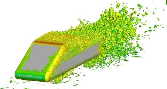
The general flow structure for the three cases is compared using iso-surfaces of total pressure coefficient on
Figure 10. For the RANS simulation, the only visible flow features are the wake and barely the pair of vortices over the C-pillar. All of the other coherent structures are faded out. On the other hand, simulations based on the spectral/hp element method distinctly resolve the wake and the vortices emanating from the A-pillar and the C-pillar. The vortex originating from flow separation on the A-pillar are convected downstream along the side surfaces of the body before being deflected towards the centreplane driven by the low pressure wake. Although the resolution at which the vortices are captured is higher for the HCP5 case, they are convected further downstream in the HFP3 case. The pair of vortices generated at the top outboard edge of the slant and rolling over the trailing pillars, which have been evidenced in the shear-stress contour in
Figure 8 and by Wood et al. [
7], are well captured in high-order simulations in both cases. The same difference on the two meshes is observed for the A-pillars, with the pair of vortices being more finely resolved for the HCP5 mesh but extending further downstream for HFP3 where they merge with the wake directly downstream from the base of the vehicle. The total pressure coefficient iso-surface also confirms the larger separation on the centreplane at the beginning of the slant for the HFP3 case, which was highlighted on
Figure 6.
Figure 11 shows the progression of vorticity magnitude over the SAE body with both the HCP5 and the HFP3 meshes. The results shown in the total pressure coefficient iso-surfaces in
Figure 10 are also confirmed by these vorticity contours. Looking at the
planes, the HCP5 mesh looks asymmetric with additional vortex rollup over the left-hand side of the body than the right, whilst the positioning of the rollup in HFP3 is slightly asymmetric—the number and intensity of the roll-up look similar on both sides of the car. The difference here can be due to the shorter averaging period for HCP5, preventing the capture of low-frequency asymmetric vortex shedding from the left- and right-hand sides of the vehicle. This trend also exists in the
plane. The layer of high vorticity values near the surface on the top corners of the vehicle evolved in distinct vortices. The strength of the vortices looks somewhat higher in HFP3 even if the vortices can be distinguished with better resolution in the HCP5 case. Further downstream at
, most of the vortices generated at the A-pillar vanished in the HCP5 case, whereas they are still visible on at this streamwise location for HFP3 with lower vorticity levels. The asymmetry could point towards the possibly of bi-stability in the wake dynamics of the SAE-body at this Reynolds number—however, the possibility of this is left for further investigations.
The backlight dynamics mimic what was seen in
Figure 10. The propagation of the stronger A-pillar vortex results in the counter-rotating vortex pair that can be seen over both C-pillars in the
plane in the HFP3 case. The system looks decidedly weaker in the HCP5 case with no counter-rotating vortex core interaction with the diffusion of the A-pillar vortex core upstream from the backlight. The pair of vortices rolling over the trailing pillars are captured on both cases just above the backlight surface. Both wakes look much more symmetric in both cases, suggesting that any bi-stability in the A-pillar vortex cores may have limited implications on the vortex system over the backlight and any wake dynamics or overall forces.
6. Implications and Suggested Further Work
This study demonstrates the potential shortcomings of current mesh best practices with regard to high-order methodologies and hybrid h/p-type approaches. Whilst retaining a similar number of total degrees of freedom between the two meshes, fairly significant differences in both general flow structures can be seen in the presented figures above. In particular, the complex vortical interactions between the A- and C-pillars differ greatly between the two different meshes.
The results show that RANS simulations perform very well on this simplified vehicle, especially for time-averaged surface pressure distributions. However, it fails at accurately resolving complex off-body flow structures such as the leading and trailing vortices, which are captured by the scale resolving simulations with Nektar++. This is observed, to a lower extent, on the wake length prediction, which is overestimated in the RANS simulation. The curved junction between the roof and the backlight turns out to be the most problematic region. The wall models of the RANS simulations accurately predict attached flow for this particular situation, whereas separated flow appears in scale-resolving simulations. This could partly be explained by the lack of turbulence in the incoming flow compared with RANS modelling, which supposes a fixed amount on inlet turbulence. The difference in the size of the separation bubble at the centreplane between HCP5 and HFP3 indicates that h- and p-resolutions also have an influence over the flow pattern in this region. Accurate prediction of the flow over this geometric feature requires fine resolution near the wall to accurately predict the interaction between the boundary layer and pressure gradient. Indeed, SGS are dampened by the SVV. The energy deficit coming from unresolved scales causes early separation of the boundary layer by making it more difficult to withstand adverse pressure gradients. The smaller separation over the top of the backlight obtained with the HCP5 simulation at this location tends to indicate that p-type refinement is to be favoured to increase the near-wall resolution. In fact, a previous Eigensolution analysis performed on advection-diffusion equations by Moura et al. [
17,
18] showed that the additional viscosity strongly impacts higher-order modes corresponding to small scales while preserving smaller scales. Therefore, large and intermediate scales carrying the bulk of the turbulent kinetic energy remain relatively less affected by the additional diffusion introduced by the SVV in the HCP5 case than HFP3, which is of a lower order.
Whilst resolved structures seemed to be better defined in the case of higher polynomial order simulation, the finer h mesh seemed to resolve overall more vorticity and allowed vortices to be tracked over longer distances. This observation suggests that a trade-off has to be found between h- and p-type refinements for off-body flow features. Indeed, sufficient mesh refinement has to be prescribed for the linear mesh to be able to capture flow features and to propagate them over a long distance. Once the linear mesh has been set, the polynomial order can be gradually increased to improve their resolution. However, it has to be kept in mind that raising the polynomial order is accompanied by a large increase in the total number of degrees of freedom. For instance, going from a second order polynomial approximation to a third order more than doubles the total number of degrees of freedom, and a trade-off has to be made between computational resources and turbulent scale resolutions. Some further work on hybrid meshes and meshing best practices are needed to ensure the robustness of these methodologies. Further investigations with regards to the boundary layer resolution and wider free-stream requirements could be assessed in studies moving forward. For instance, canonical mesh sweeps of both differing h- and p-strategies could lead to further insight with regards to the questions raised in this report. Further simulations on complex geometries, such as the SAE body, could also be conducted to ensure that these results are consistent with industrial geometries.
7. Conclusions
Hybrid high-order approaches utilising both h- and p-type refinement show promise in aerodynamic applications, particularly when discussing scale-resolving techniques such as Large-Eddy Simulation and Direct Numerical Simulation. Due to these techniques being in their infancy in comparison with more traditional and widely adopted approaches such as Finite-Volume and linear Finite-Element, the accepted best-practices for traditional techniques seem to be less applicable to high-order methods. The results above show significant differences in the resolved vorticity, flow structures and surface pressure over the SAE body for the same targeted degrees of freedom. These results lay the basis for the generation of high-order meshes for complex industrial cases and, as discussed, show the need for further work investigating the requirements for these hybrid techniques and briefly sets out how this could be achieved.
Author Contributions
Conceptualization, W.H., J.S. and F.F.B.; methodology, W.H., J.S. and F.F.B.; software, S.S.; validation, W.H., J.S. and F.F.B.; formal analysis, W.H., J.S. and F.F.B.; investigation, W.H., J.S. and F.F.B.; resources, S.S.; data curation, W.H., J.S. and F.F.B.; writing—original draft preparation, W.H., J.S. and F.F.B.; writing—review and editing, W.H., J.S., F.F.B. and S.S.; visualization, W.H., J.S. and F.F.B.; supervision, S.S.; project administration, S.S. All authors have read and agreed to the published version of the manuscript.
Funding
This research received no external funding.
Data Availability Statement
Acknowledgments
The authors acknowledge the Cambridge CSD3 HPC service for the use of their computational resources in completing this study.
Conflicts of Interest
The authors declare no conflict of interest.
References
- Ahmed, S.; Ramm, G.; Faltin, G. Some Salient Features of the Time-Averaged Ground Vehicle Wake; Technical Report, SAE Technical Paper; SAE: Warrendale, PA, USA, 1984. [Google Scholar]
- Howell, J.; Sheppard, A.; Blakemore, A. Aerodynamic Drag Reduction for a Simple Bluff Body Using Base Bleed; Technical Report, SAE Technical Paper; SAE: Warrendale, PA, USA, 2003. [Google Scholar]
- Cogotti, A. A parametric study on the ground effect of a simplified car model. SAE Transact. 1998, 107, 180–204. [Google Scholar]
- Basara, B.; Przulj, V.; Tibaut, P. On the Calculation of External Aerodynamics: Industrial Benchmarks; SAE Technical Paper Series; SAE: Warrendale, PA, USA, 2001. [Google Scholar] [CrossRef]
- Ishima, T.; Takahashi, Y.; Okado, H.; Baba, Y.; Obokata, T. 3D-PIV Measurement and Visualization of Streamlines Around a Standard SAE Vehicle Model; SAE Technical Paper Series; SAE: Warrendale, PA, USA, 2011. [Google Scholar] [CrossRef]
- Nader, A.; Islam, A.; Thornber, B. A Comparative Aerodynamic Investigation of a 20° SAE Notchback Model. Appl. Mech. Mater. 2016, 846, 79–84. [Google Scholar] [CrossRef]
- Wood, D.; Passmore, M.; Perry, A. Experimental data for the validation of numerical methods-SAE reference notchback model. SAE Int. J. Passeng. Cars-Mech. Syst. 2014, 7, 145–154. [Google Scholar] [CrossRef] [Green Version]
- Buscariolo, F.F.; Hoessler, J.; Moxey, D.; Jassim, A.; Gouder, K.; Basley, J.; Murai, Y.; Assi, G.R.; Sherwin, S.J. Spectral/hp element simulation of flow past a Formula One front wing: Validation against experiments. J. Wind Eng. Ind. Aerodyn. 2022, 221, 104832. [Google Scholar] [CrossRef]
- Buscariolo, F.; Assi, G.; Meneghini, J.; Sherwin, S. Spectral/hp methodology study for iLES-SVV on an Ahmed Body. In Spectral and High Order Methods for Partial Differential Equations ICOSAHOM 2018; Springer: Berlin/Heidelberg, Germany, 2020. [Google Scholar]
- Mengaldo, G.; Moxey, D.; Turner, M.; Moura, R.C.; Jassim, A.; Taylor, M.; Peiro, J.; Sherwin, S.J. Industry-Relevant Implicit Large-Eddy Simulation of a High-Performance Road Car via Spectral/hp Element Methods. arXiv 2020, arXiv:cs.CE/2009.10178. [Google Scholar] [CrossRef]
- Cantwell, C.; Moxey, D.; Comerford, A.; Bolis, A.; Rocco, G.; Mengaldo, G.; Grazia, D.D.; Yakovlev, S.; Lombard, J.E.; Ekelschot, D.; et al. Nektar++: An open-source spectral/hp element framework. Comput. Phys. Commun. 2015, 192, 205–219. [Google Scholar] [CrossRef] [Green Version]
- Karniadakis, G.; Sherwin, S. Spectral/hp Element Methods for Computational Fluid Dynamics; Oxford University Press: Oxford, UK, 2005. [Google Scholar] [CrossRef]
- Vermeire, B.C.; Witherden, F.D.; Vincent, P.E. On the utility of GPU accelerated high-order methods for unsteady flow simulations: A comparison with industry-standard tools. J. Comput. Phys. 2017, 334, 497–521. [Google Scholar] [CrossRef]
- Jiang, H.; Cheng, L. Large-eddy simulation of flow past a circular cylinder for Reynolds numbers 400 to 3900. Phys. Fluids 2021, 33, 034119. [Google Scholar] [CrossRef]
- Buscariolo, F.; Assi, G.; Sherwin, S. Computational study on an Ahmed Body equipped with simplified underbody diffuser. J. Wind Eng. Ind. Aerodyn. 2021, 209, 104411. [Google Scholar] [CrossRef]
- Guermond, J.L.; Shen, J. Velocity-correction projection methods for incompressible flows. SIAM J. Numer. Anal. 2003, 41, 112–134. [Google Scholar] [CrossRef]
- Moura, R.; Sherwin, S.; Peiró, J. Eigensolution analysis of spectral/hp continuous Galerkin approximations to advection–diffusion problems: Insights into spectral vanishing viscosity. J. Comput. Phys. 2016, 307, 401–422. [Google Scholar] [CrossRef] [Green Version]
- Moura, R.C.; Mengaldo, G.; Peiró, J.; Sherwin, S.J. On the eddy-resolving capability of high-order discontinuous Galerkin approaches to implicit LES/under-resolved DNS of Euler turbulence. J. Comput. Phys. 2017, 330, 615–623. [Google Scholar] [CrossRef] [Green Version]
- Moxey, D.; Green, M.D.; Sherwin, S.J.; Peiró, J. An isoparametric approach to high-order curvilinear boundary-layer meshing. Comput. Methods Appl. Mech. Eng. 2015, 283, 636–650. [Google Scholar] [CrossRef] [Green Version]
- Dong, S.; Karniadakis, G.; Chryssostomidis, C. A robust and accurate outflow boundary condition for incompressible flow simulations on severely-truncated unbounded domains. J. Comput. Phys. 2014, 261, 83–105. [Google Scholar] [CrossRef]
| Publisher’s Note: MDPI stays neutral with regard to jurisdictional claims in published maps and institutional affiliations. |
© 2022 by the authors. Licensee MDPI, Basel, Switzerland. This article is an open access article distributed under the terms and conditions of the Creative Commons Attribution (CC BY) license (https://creativecommons.org/licenses/by/4.0/).


