Machine Learning on Fault Diagnosis in Wind Turbines

Abstract

With the improvement in wind turbine (WT) operation and maintenance (O&M) technologies and the rise of O&M cost, fault diagnostics in WTs based on a supervisory control and data acquisition (SCADA) system has become among the cheapest and easiest methods to detect faults in WTs.Hence, it is necessary to monitor the change in real-time parameters from the WT and maintenance action could be taken in advance before any major failures. Therefore, SCADA-driven fault diagnosis in WT based on machine learning algorithms has been proposed in this study by comparing the performance of three different machine learning algorithms, namely k-nearest neighbors (kNN) with a bagging regressor, extreme gradient boosting (XGBoost) and an artificial neural network (ANN) on condition monitoring of gearbox oil sump temperature. Further, this study also compared the performance of two different feature selection methods, namely the Pearson correlation coefficient (PCC) and principal component analysis (PCA), and three hyperparameter optimization methods on optimizing the performance of the models, namely a grid search, a random search and Bayesian optimization. A total of 3 years of SCADA data on WTs located in France have been used to verify the selected method. The results showed the kNN with a bagging regressor, with PCA and a grid search, provides the best R² score, and the lowest root mean square error (RMSE). The trained model can detect the potential of WT faults at least 4 weeks in advance. However, the proposed kNN model in this study can be trained with the Support Vector Machine hybrid algorithm to improve its performance and reduce fault alarm.

1. Introduction

Wind energy is among the most important renewable energies. In 2021, the installation of offshore wind turbine plants was 3-fold greater than in 2020 and this increased the global power output from wind power plants to 837 GW, showing a growth of 12% compared to 2020 [1]. The wind energy industry has been growing drastically lately as governments all around the world understand the importance of wind energy in achieving the target of 1.5 °C global warming by 2100 set by the Paris Agreement [2]. A total 557 GW of wind power output is expected to be achieved by 2026 [1]. Further, BloombergNEF (BNEF) forecasted that global offshore WT capacity will reach 5.3 GW by 2030 [3]. The Global Energy Wind Council stated that the wind energy industry needs to scale up annual wind turbine plant installation by 4 fold to meet the global warming target of 1.5 °C [1].

However, the wind energy industry is facing higher operation and maintenance (O&M) costs and unplanned replacement costs amid uncertainties. O&M costs are expected to grow 8% annually by 2025, from USD 13.7 billion in 2016 to an estimated USD 27.4 billion in 2025 [4]. Figure 1 shows that the O&M cost took up to 21% of the total cost in a wind turbine project [5].

The cost of unplanned maintenance is significantly high as well.

Table 1. Subsystem Replacement Cost of a 5 MW Offshore Wind Turbine [5].

Name of Subsystem	Cost (DKK)
Gearbox	3,937,000
Generator	1,968,000
Blade	1,625,000

shows the cost of replacement of three different subsystems in an offshore WT. The replacement cost of a gearbox is double the cost of a generator or blade as replacements for such systems require a vessel and crane [5].

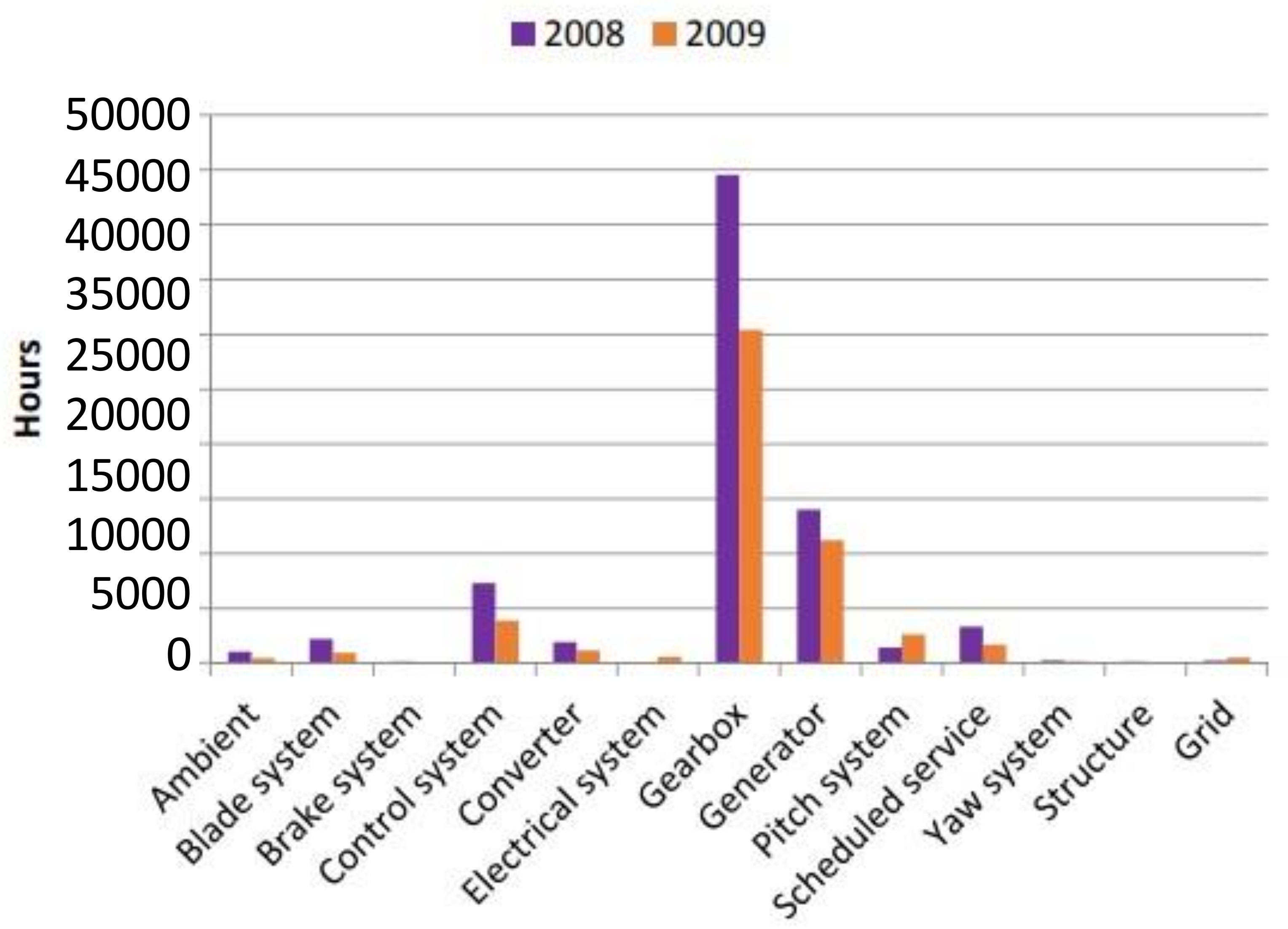
Virus outbreaks and tensions between countries are resulting in financial stress in the wind energy industry due to the rise in the prices of key materials and logistics. The price of future projects in wind energy plants will remain high in 2022 according to a BNEF report [3]. Further, wind plant operators will face higher costs and lower profits when unscheduled maintenance occur due to long downtimes as major parts such as generators and gearboxes require longer downtimes for maintenance and repair. Figure 2 showed that gearboxes and generators cause the longest downtime for WTs.

BNEF stated that a series of wind turbine faults in the past could lead to greater turbine faults in the future [3]. Hence, it is important to analyze and study the behavior of wind turbine plants so as to avoid any unnecessary costs by developing a condition monitoring system (CM) based on Supervisory Control and Data Acquisition (SCADA) data such as wind speed, gearbox bearing temperature, and generator bearing temperature.

CMs help to take effective advanced maintenance action by detecting any impending faults in WTs. CMs can help to save up to 25% of maintenance costs compared with scheduled maintenance costs [6]. CMs can constitute applying machine learning on the SCADA data collected by sensors in WTs. Machine learning could study the behavior of WTs and it is possible to detect if a fault is developing in WTs. The term machine learning was created by Arthur Samuel in 1959 while at IBM [7]. Machine learning is a branch of artificial intelligence and computer science which applies an algorithm network on a set of data to model what humans learn [8]. Machines are able to solve issues or provide signals based on what they learn. However, according to Alpaydn, to solve a problem on a computer, an algorithm is needed [9]. Machine learning algorithms are publicly available and include TensorFlow [10] and PyTorch [11]. Machine learning has been widely used in different industries such as the medical [12], food and beverage [13], construction [14] and renewable energy fields [15]. The SCADA data have been used to detect potential catastrophic failures in wind turbines by applying a regression model [16]. A study showed that a bagging regressor managed to achieve a early fault alarm 9 days earlier than the actual failure without stating the computational time required by the proposed method [17]. Studies have proven the efficiency of machine learning on fault diagnosis in wind turbines, but the computation times of different machine learning models were not highly emphasized although this is among the main factors of model selection as computation time will affect the setup cost and computation resources. Further, data pre-processing methods have not been studied together with the performance of different machine learning models.

Therefore, the purpose of this study is to determine an algorithm network to diagnose fault patterns on gearbox oil sump temperature in WTs. Three different machine learning algorithms, K-nearest neighbor (kNN) with a bagging regressor algorithm, the extreme gradient boosting (XGBoost) algorithm and an artificial neural network (ANN), will be applied in this study and their performance and computational time will be compared and discussed. The algorithm with the best performance in terms of the lowest root mean square error (RMSE) and the highest R² score will be chosen to train the condition monitoring model. Further, feature selection methods, namely the Pearson correlation coefficient and principal component analysis, and hyperparameter optimization methods, namely a grid search, a random search and Bayesian optimization, will be applied in this study and their results will be discussed. A set of SCADA wind turbine data from ENGIE, a wind turbine operator, will be used to train the three algorithm networks.

2. Machine Learning Model

2.1. Resources Used

The hardware and software used in this study are shown in

Table 2. Hardware Configuration of Equipment Used.

Equipment	Hardware Configuration
Laptop	Lenovo IdeaPad Gaming 3 15ACH6
Processor	AMD Ryzen 5 5600H with Radeon Graphics 3.30 GHz
RAM	8.00 GB
System type	64-bit operating system

and

Table 3. Software Configuration.

Software	Software Configuration
Laptop	Windows 10 Home OS 19044.2006
Programming Tool	Anaconda Jupyter Notebook Version 6.1.4

, respectively.

The SCADA data in this study were obtained from a WT farm operated by Engie at La Houte Borne, France [18]. There were a total of four different wind turbines, of the MM82 model, manufactured by Senvion and labelled as R80721, R80736, R80790 and R80711. The rated power of each WT at the WT farm is 2050 kW. The wind turbine has a rotor with a diameter of 82 m and a hub at a height of 80 m. The SCADA data were collected from the wind turbine at an interval of 10 min from 2013 to 2016. Due to insufficient computational memory space in this study, data for 2013 were removed. There were a total of 34 parameters captured from the WTs, as shown in

Table 4. Description of WT operation variables [18].

Variable Name	Variable Long Name	Unit	Comment
Ba	Pitch angle	deg
Cm	Converter torque	Nm
Cosphi	Power factor		Should equal P/S
DCs	Generator converter speed	rpm
Db1t	Generator bearing 1 temperature	deg C
Db2t	Generator bearing 2 temperature	deg C
Ds	Generator speed	rpm
Dst	Generator stator temperature	deg C
Gb1t	Gearbox bearing 1 temperature	deg C
Gb2t	Gearbox bearing 2 temperature	deg C
Git	Gearbox inlet temperature	deg C
Gost	Gearbox oil sump temperature	deg C
Na c	Nacelle angle corrected	deg
Nf	Grid frequency	Hz
Nu	Grid voltage	V
Ot	Outdoor temperature	deg C
P	Active power	kW
Pas	Pitch angle setpoint
Q	Reactive power	kVAr
Rbt	Rotor bearing temperature	deg C
Rm	Torque	Nm
Rs	Rotor speed	rpm
Rt	Hub temperature	deg C
S	Apparent power	kVA	Should be the square root of the sum of P square and Q square
Va	Vane position	deg
Va1	Vane position 1	deg	First wind vane on the nacelle
Va2	Vane position 2	deg	Second wind vane on the nacelle
Wa	Absolute wind direction	deg
Wa c	Absolute wind direction corrected	deg
Ws	Wind speed	m/s	Average wind speed
Ws1	Wind speed 1	m/s	First anemometer on the nacelle
Ws2	Wind speed 2	m/s	Second anemometer on the nacelle
Ya	Nacelle angle	deg
Yt	Nacelle temperature	deg C

.

The International Electrotechnical Commission presented a list of parameters to be collected in the SCADA system from each working wind turbine but not all operators follow [19], hence, the parameters collected from different operators varied [20,21]. Parameters other than those listed by the International Electrotechnical Commission were filtered out [19], leaving a are total of 17 parameters for use in this study—DCs, Db1t, Db2t, Ds, Dst, Gb1t, Gb2t, Git, Gost, Ws1, Ws2, Ws, Rs, S, P, Q and Rbt. Furthermore, only average values are used in this study. Data with non-numerical values were removed as well. The average values of all the parameters are used in this study, as the minimum value, the maximum value and the standard deviation value of the SCADA were removed.

2.2. Processing of Outliers

It is important to eliminate outliers in the SCADA data for accuracy and reliability of the trained model. Next, abnormal points in the SCADA data such as a power of 0, a wind speed of 0 or a negative wind speed were removed. A power curve is used as a reference for the expected behavior of WTs, as shown in Figure 3. The power curve shows that the relationship between WT power and wind speed. The cut-in speed of the WTs in La Houte Borne WT Farm is 4 m/s, the rated wind speed is 14.5 m/s and the cut-out wind speed is 22 m/s.

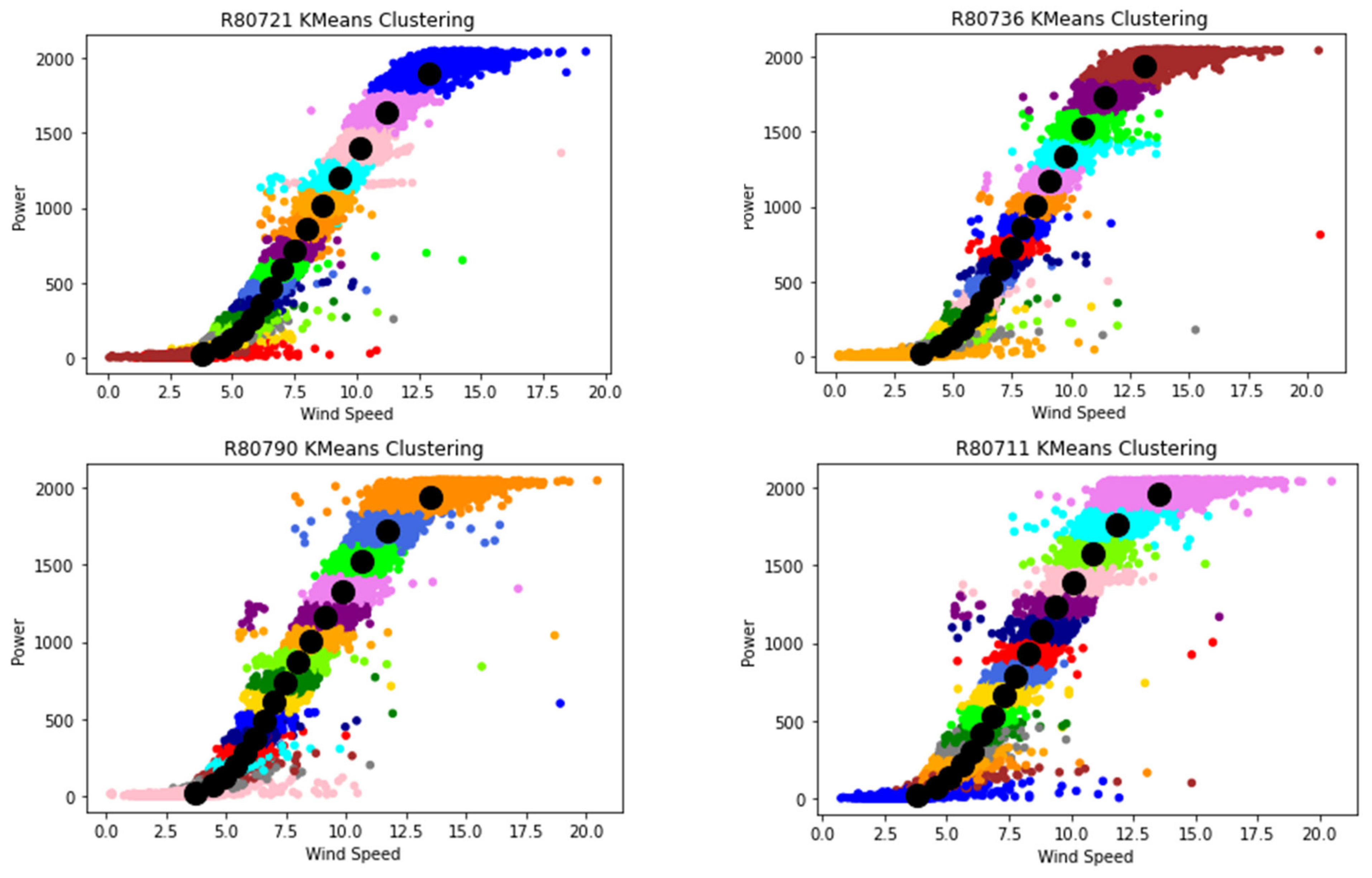
K-mean clustering is applied in this study. K-mean clustering was first proposed in 1987 [22]. The K-means elbow method is used to identify the number of clusters by plotting the number of clusters versus the sum of squares within a cluster. The sum of squares within a cluster is a measure of the variability of the observation made within a cluster [23]. A number of clusters greater than 7 is safe to use as the K means begins to stabilize at K means clusters of 7, as shown in Figure 4. K-means clustering with 16 clusters is used to identify all the clusters in wind speed data with power output, the within-cluster sum of squares begins to stabilize at clusters of 16, as shown in Figure 4, with the lowest variability of the observations made within each clusters. The Mahalanobis distance (MD) is used to eliminate all the anomalies by applying Equation (1) [24]. The points with a higher MD will be removed as they are identified anomalies because the distances between the points and the center of the clusters are greater than the mean distance of all the points in the cluster.

$$M{D}_i=\left(x_i-\overline{x}\right)C_x^{-1}{\left(x_i-\overline{x}\right)}^T$$

(1)

where $x$ is the data variable, $\overline{x}$ is the mean data variable and $C_x^{}$ is the variance covariance matrix of data x. $C_x^{}$ is calculated by using Equation (2) [24]

$$C_x=\left[\begin{array}{cc}{\sigma }_1^2& {\rho }_{12}{\sigma }_1{\sigma }_2\\ {\rho }_{12}{\sigma }_1{\sigma }_2& {\sigma }_2^2\end{array}\right]$$

(2)

where ${\sigma }_1^2$ and ${\sigma }_2^2$ are the variances of the first and second variables and ${\rho }_{12}{\sigma }_1{\sigma }_2$ is the covariance between two variables.

2.3. Method for Selection of Features

For selection of features, the Pearson correlation coefficient (PCC) is used in this study to determine the correlation between two features X and Y [25,26]. PCC can be determined by applying Equation (3). PCC ranges from 1 to −1, where 1 means that X and Y are correlated to each other positively and -1 means that X and Y are correlated to each other negatively [26]. Likewise, 0 means that X and Y are not correlated to each other [25]. X and Y have a strong correlation when PCC is greater than 0.8 [26].

Highly correlated features are removed from the dataset because this is helpful to improve the accuracy of the trained model and reduce overfitting to some extent. This is a statistical phenomenon called multicollinearity, where the variables are highly correlated to each other [27]. Highly correlated features will cause inaccurate variances, resulting in unstable prediction by the trained model. Hence, removal of highly correlated features could help to reduce the effect of multicollinearity on the trained model.

Highly correlated features are removed at the set threshold of 0.95 as this provides the best result in terms of accuracy, where 0.9 to 1.0 are considered very highly correlated [28].

$${\rho }_{X,Y}=\frac{COV \left(X,Y\right)}{{\sigma }_X{\sigma }_Y}$$

(3)

where COV(X,Y) is the covariance of X and Y, ${\sigma }_X$ and ${\sigma }_Y$ are the variances of X and Y features, respectively.

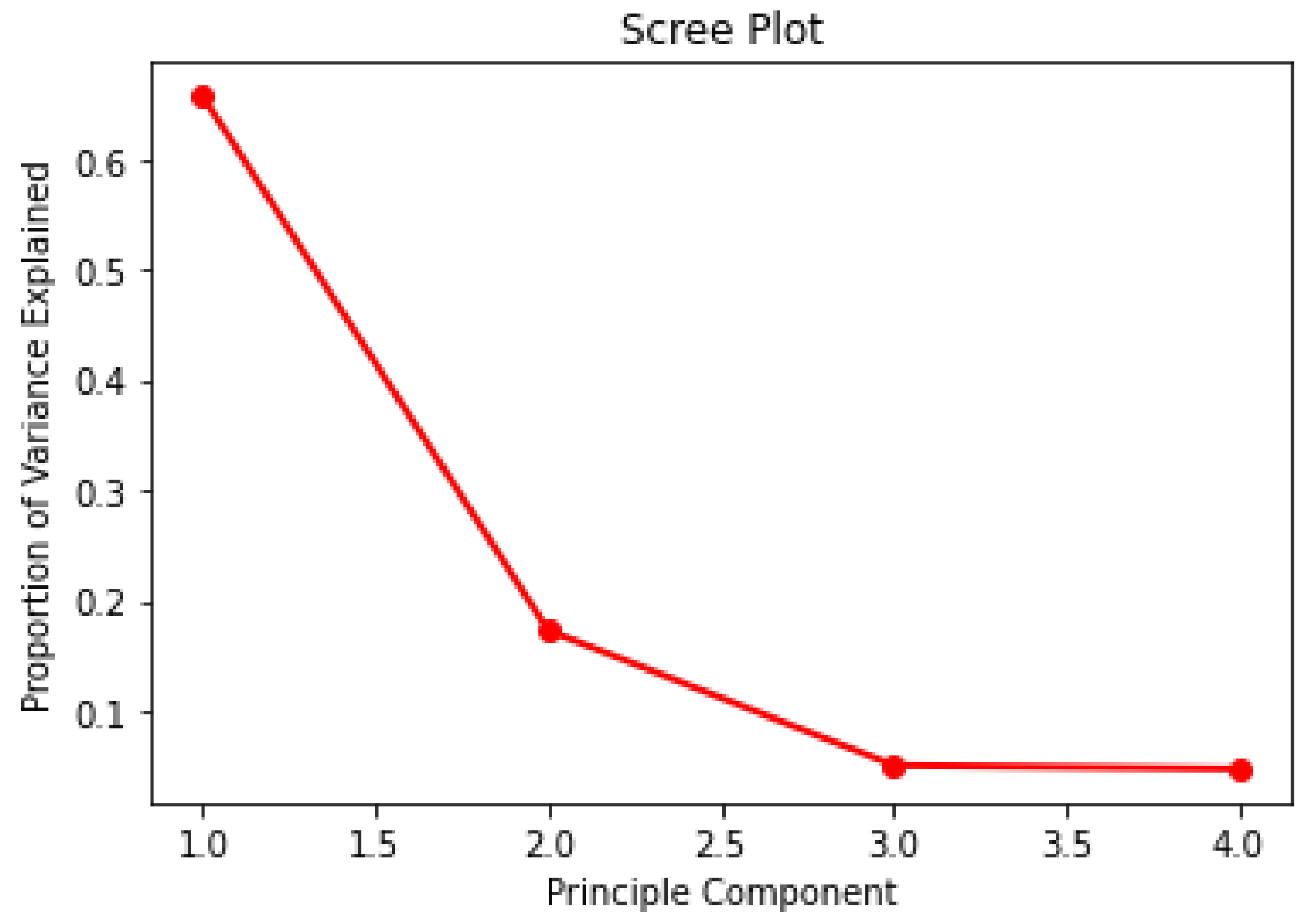
Principal component analysis (PCA) is also used in this study to determine the important features. PCA is a mathematical tool used to represent the variation of features in a dataset by using a small number of factors. The 2D or 3D projection of samples is shown by setting the axes (principal components, PCs) as the factors [29]. Principle components are constructed in such a sequence, where the first principle component (PC1) holds on to the largest possible variance in the dataset. The second principle component (PC2) holds the largest possible variance among all the remaining combinations, given that PC2 is not correlated with PC1. The subsequent principle components are designed in a similar way. The number of principle components is identified by using a scree plot, as illustrated in Figure 5.

A scree plot shows the proportion of variance explained vs. the principle component. The ‘elbow’ is set at PC = 3 as the proportion of variance explained plateaus after PC = 3. Hence, 4 principle components are taken into consideration in this study.

2.4. Hyperparameter Optimization

The main objective of a machine learning algorithm is to minimize loss function given a set of parameters. A good machine learning algorithm produces an optimized function by selecting all the correct hyperparameters. The process to determine a set of good hyperparameters is called hyperparameter optimization. Hyperparameter optimization is performed in this study by applying a grid search [30], a random search [31] and Bayesian optimization [32]. In a grid search, the algorithm will search through a fixed domain of hyperparameters. Therefore, a grid search will consume more computational sources and time when there are more hyperparameters. A random search will search within a range of hyperparameters randomly with limited computation resources. The Bayesian optimization algorithm will eliminate hyperparameters if the outcome is worse than the previous one, hence it will save more computational resources and time.

2.5. Machine Learning Algorithms

There are three different algorithms used in this study, k-nearest neighbor (kNN) with a bagging regressor, a tree ensemble with extreme gradient boosting (XGBoost) and an artificial neural network (ANN), which will be explained in the next section. KNN with a bagging regressor and XGBoost are easily available in the Python Scikit-learn library [33]. The datasets from WTs R80721, R80736, and R80711 are used as the training dataset [18]. The dataset from R80790 is used as the testing dataset [18].

2.5.1. K-Nearest Neighbor with a Bagging Regressor

K-nearest neighbor (kNN) is a supervised machine learning model that deduces a function from a training sample dataset [34]. kNN is simple and easy to understand and can be applied to regression and classification problems but it has a major drawback that will be discussed in a later section. Each sample in the dataset has an input vector and a desired output value. After the model is trained using the training dataset, the trained model will be used to determine the output for any given dataset.

The training dataset has n samples and each sample $x_i$ is described by k input variables and an output variable $y_i$ such that $x_i=\left\{x_1,x_2,\dots , x_k,y_i\right\}.$ The goal is to minimize the distance function that determines the relationship between input variables and output variables. The distance functions could be Euclidean Distance or Manhattan Distance, as shown in Equations (4) and (5), respectively.

$$Euclidean Distance=\sqrt{{\displaystyle \sum }_{i=1}^k{\left(x_i-y_i\right)}^2}$$

(4)

$$Manhattan Distance={\displaystyle \sum }_{i=1}^k\left|x_i-y_i\right|$$

(5)

Once the distance from the points in the training set have been measured, the model will look for the new point that gives the nearest distance between k nearest points. The value of k will be used to determine the number of points being measured during training. Hence, it is crucial to determine the value of k [35]. A large k will reduce the noise and minimize the prediction loss, but will increase the computational cost and time if a large training dataset is used; however, a small k will simplify the prediction process and reduce computational cost. Hence, the computational time for kNN will become shorter as the size of the dataset grows.

Validation error is used to determine the value of k to be used in a kNN regressor. A value of 6 is chosen as the number of k-neighbors in the kNN regressor as the RMSE plateaus after reaching 6, as shown in Figure 6.

Next, a bagging tree (BT) regressor is used to improve on the kNN regressor. In a BT regressor, multiple data subsets, D_i, are constructed from the training dataset from the kNN regressor by sampling randomly with replacement and without pruning [36]. This is the bootstrap method. These bootstraps will eventually be used to construct a single regression tree. All individual trees are then combined in an ensemble. Hence, this method is also called the tree ensemble method. The predicted outcome will be averaged over all the trees, as shown in Figure 7 [37]. Therefore, a BT regressor helped to improve the accuracy of the trained model by reducing the variance or errors.

To achieve optimal performance, the hyperparameters of kNN regressor-like k-neighbors, a distance function and weight must be tuned by using the three optimization methods: a grid search, a random search and Bayesian optimization. The one with the best performance will be used in the bagging regressor. The tuning space of the hyperparameters is shown in

Table 5. Tuning Space for Hyperparameters in the kNN model.

Hyperparameters	Tuning Space
K-neighbors	1 to 50
Distance function	Euclidean and Manhattan Distance Functions
Weight	Uniform and Distance

.

2.5.2. A Regressor Tree Ensemble with eXtreme Gradient Boosting

XGBoost has been developed by Chen and He [38]. XGBoost is a scalable end-to-end gradient tree boosting system. The gradient tree boosting technique is introduced by JH Friedman [39]. Firstly, in a tree regressor model, an objective function is tasked to be minimized by selecting a set of correct parameters $\theta$. An objective function can be defined as Equation (6) [40].

$$Obj={\displaystyle \sum }_{i=1}^{n}L\left(y_{xi}{\widehat{y}}_{xi}\right)+{\displaystyle \sum }_{m=1}^M\mathsf{\Omega }{\left(f_m\right)}_{ }$$

(6)

where n is the sample size, L is a second-order derivable loss function which calculates the difference between the actual target variable, $y_{xi}$, and the predicted target variable, ${\widehat{y}}_{xi},$ $\mathsf{\Omega }\left(f_m\right)$ is the regularization term, M denotes the number of trees in the trained model and m is the m-th tree. A regularization term helped us to avoid overfitting the model. $\mathsf{\Omega }\left(f_m\right),$a regularization term, is calculated by Equation (7) [40].

$$\mathsf{\Omega }\left(f_m\right)=\gamma T+\frac{1}{2}\beta {\displaystyle \sum }_{j=1}^T{w}_j^2$$

(7)

where $T$ is the number of leaf nodes in the tree, $w_j^{}$ is the score of each leaf node, and $\gamma$ and $\beta$ are the hyperparameters to control the complexity of the tree. $\gamma$ and $\beta$ will be represented by alpha and lambda in the XGBoost algorithm provided by SKLearn [33]. They will be set as 0 by default. The tuning space for alpha and lambda will be provided in

Table 6. Tuning Space for Hyperparameters in the XGBoost Model.

Hyperparameters	Tuning Space
Max depth	15, 20
Lambda value	0.1, 0.5
Alpha value	0.1, 0.5
Number of estimator	750, 800
Subsample ratio of each column when constructing each tree	0.5, 0.9

.

The prediction score will be assigned to each of the leaves in a tree regressor model, but a single tree is not strong enough to be used in practice. Hence, a tree ensemble is applied to sum up all the prediction scores of multiple trees together. There is a difference between boosting and bagging, boosting is an iterative technique that improves the prediction score of the next tree by adjusting the weight based on the last prediction score, as explained in Figure 8 [41]; likewise, bagging reduces the variance error by constructing multiple trees and taking the average prediction score of all trees. The gradient descent algorithm is used in XGBoost to minimize our objective function or the loss function [42]. The gradient descent algorithm is a first-order iterative optimization algorithm to find the local minimum of a given differentiable function [43]. There are two requirements for the function to be used in a gradient descent algorithm, and the function has to be differentiable and needs to give a convex curve [44].

It is very important to select the correct hyperparameters for use in the XGBoost model as they will affect the model significantly [40]. The hyperparameter tuning space for the XGBoost model is shown in Table 6.

Due to the limited computation resources, there was limited tuning space for hyperparameters in the XGBoost model. Other hyperparameters were selected by a random search in advance, as shown in

Table 7. Fixed Hyperparameters in XGBoost Model.

Hyperparameters	Value
Booster	Gradient boosting tree
Sample ratio for each level	0
Sample ratio for each tree	0
Gamma value	3
Learning rate	0.1
Maximum depth of tree	3
Random state	30

, as the random search used a shorter computational time and less computational resources.

2.5.3. The Artificial Neural Network

Artificial neural networks (ANNs) are a branch of artificial intelligence. S. Haykin [45] stated that an ANN is a machine that works similar to a human brain to perform a given task of interest. An ANN is considered as a deep learning method that utilizes a neural network to perform similar to a human brain. The human brain consists of many interconnected ‘neurons’ and they are trained to perform tasks on a daily basis such as recognizing speech, recognizing an image, and processing language. ANNs can learn similar to how human brains work. ANNs have been used extensively in applications to recognize language, analyze texture, recognize facial expressions, detect undersea activity and detect faults in machine.

ANNs consist of multilayer perceptrons and form a neural network that consists of an input layer, hidden layers and output layers, with interconnected neurons or nodes, as shown in Figure 9 [46]. The nodes are represented as weights and output signals with transfer functions of the sum of the input signal modified by a simple nonlinear activation function, as shown in Figure 10. Superposition of nonlinear functions is implemented to simplify the multilayer perceptron system [47]. Hence, ANNs are commonly applied now due to their high adaptivity and nonlinearity.

Two hidden layers are used in this study. Various numbers of nodes for hidden layers 1 and 2 are applied in this study and the obtained results are compared and analyzed. The range in the number of nodes is from 5 to 20. The best results obtained from the selected number of nodes are applied in this study. Hence, hidden layer 1 was set as 18 nodes and hidden layer 2 was set as 9 nodes. The tuning space for hyperparameters is shown in

Table 8. Tuning Space for Hyperparameters in the ANN model.

Hyperparameters	Tuning Space
Activation function	‘relu’, ‘linear’
Epochs	25, 40, 55
Batch size	32, 42, 50
Initiate mode	‘uniform’, ‘normal’

.

2.5.4. Performance Evaluation

R-squared (R²) score and the root mean square error (RMSE) were used to evaluate the performance of the machine learning algorithm network. The R² score measures how well a model can predict future data by using Equation (8) [49]. The best R² score is 1. The greater the R² score, the better the performance of the model is.

$$R^2=1-\frac{{{\displaystyle \sum }}_{i=1}^N{\left(y_i-\widehat{y_i}\right)}^2}{{{\displaystyle \sum }}_{i=1}^N{\left(y_i-\overline{y}\right)}^2}$$

(8)

where $y_i$ is the observed outcome, $\overline{y}$ is the mean of the observed outcome, $\widehat{y_i}$ is the predicted outcome and N is the number of observed outcomes.

The RMSE is a measure of the dispersion of the predicted error, or the standard deviation of the predicted error. The RMSE is calculated by using Equation (9) [49].

$$RMSE=\sqrt{\frac{1}{N}{\displaystyle \sum }_{i=1}^N{\left(\widehat{y_i}-y_i\right)}^2}$$

(9)

where $y_i$ is the observed outcome, $\widehat{y_i}$ is the predicted outcome and N is the number of observed outcomes.

The RMSE and the R² score from all the three algorithms (kNN with a bagging regressor, XGBoost and ANN) are compared and they are used to determine the best algorithm network for this study.

2.5.5. Exponential Weighted Moving Average (EWMA) Control Chart

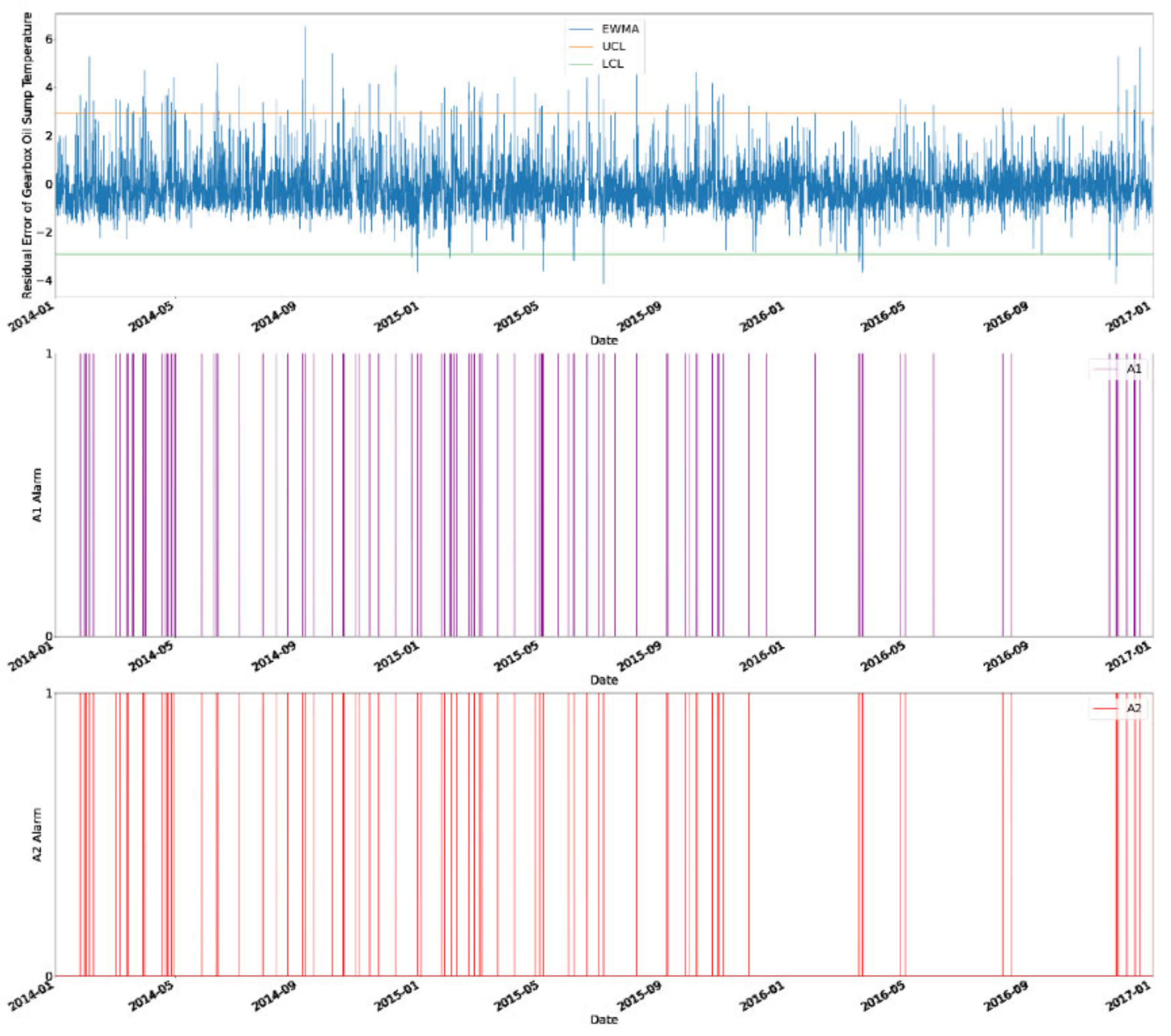
The predicted outcome from the trained model will be compared with the actual outcome. The residual error between predicted and actual outcomes will be calculated as the residual error always exists and the error is the best indicator of the health of the WT [50]. The residual error is large for unhealthy WTs, hence the magnitude of the residual error determines the condition of the WT. To determine the residual error, an EWMA chart is used [51]. An EWMA chart smoothens datasets by reducing data fluctuation. The residual error from the trained model was processed by the EWMA control chart and a lower control limit (LCL) and an upper control limit (UCL) are calculated based on the output residuals. The EWMA was calculated by Equation (10).

$$EWM{A}_t=\lambda e_t-\left(1-\lambda \right)EWM{A}_{t-1}$$

(10)

where t is the time stamp, e is residual error and $\lambda$ is a constant between 0 and 1. $\lambda$ is is set as 0.2 for this study [52].

The UCL and the LCL are calculated by Equations (11) and (12).

$$UC{L}_t=\kappa {\sigma }_e$$

(11)

$$LC{L}_t=-\kappa {\sigma }_e$$

(12)

where ${\sigma }_e$ is the standard deviation of the residual error, and $\kappa$ is a constant and set as 3 here [40].

A signal alarm system is proposed in this study by learning from a study on condition monitoring of WT [53]. There are two levels of alarms. Th first-level alarm (A1) will be triggered once the residual error is greater than the UCL or lower than the LCL. The second-level alarm (A2) will then be triggered when the first-level alarm is triggered for 3 consecutive first-level alarms, which means the abnormal condition occurred for at least 30 min as one data point is equal to a 10 min interval [53]. Binary code is applied in this signal alarm system—1 is recorded when the alarm is triggered and 0 is recorded when the alarm is not triggered. At this time, corrective actions are needed as this could be a serious problem in the WT.

An EWMA chart on generator bearing temperature in WT R80790 is used here as a reference due to an inaccessible to the fault report for WT R80790 [40].

2.6. Proposed SCADA Condition Monitoring Framework

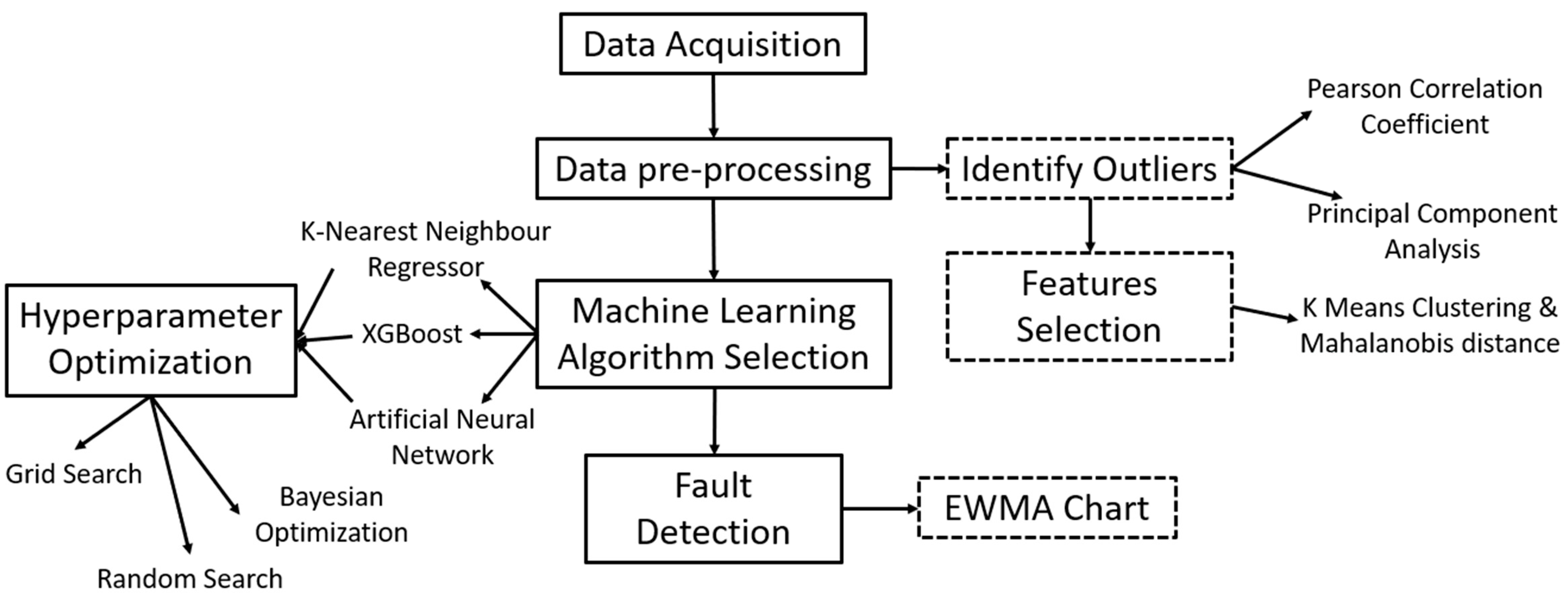
The schematic of the flow chart of the proposed condition monitoring framework is shown in Figure 11. This starts with data acquisition from the wind turbine operator, Engie. Then it follows with data pre-processing to identify outliers and features to be used in machine learning models. There are 3 different machine learning algorithms to be studied and compare based on their performance and computational time. Further, 3 different hyperparameter optimization methods are compared as well. The chosen machine learning algorithms are used to train the model in this study and the EWMA chart is applied to identify early fault alarm in WTs.

3. Result

3.1. Processing of Outliers

As mentioned in the methodology, a cluster of 16 is applied in this study because it produced the lowest variability of the observations made within each cluster to determine outliers in all the datasets from the four WTs shown in Figure 12.

After processing, the outliers were removed from the dataset. Some of the outliers were, however, not removed as the Mahalanobis distance detects outliers based on the distribution pattern of data points in each cluster. Hence, some data might be interpreted incorrectly by the Mahalanobis distance. Therefore, some of the outliers are removed manually in this study. Suggestions have been made in the conclusion part to improve the performance for the Mahalanobis distance. The graphs of wind speed vs. power for each WT are shown in Figure 13.

3.2. Feature Selection

As mentioned in the methodology, two methods were applied in this study for feature selection, namely the Pearson correlation coefficient (PCC) and principal component analysis (PCA).

3.2.1. The Pearson Correlation Coefficient

As shown in the PCC heatmap produced from this study in Figure 14, the highest value of PCC will be in dark blue color. As mentioned in the methodology, features with a coefficient of more than 0.95 are removed from this study.

There were a total of 10 variables remaining—DCs, Db1t, Db2t, Dst, Gb1t, Git, Gost, Q, Rbt and Cm—after feature selection by PCC.

Table 9. Shape of Wind Turbine Dataset after Variables Selection by PCC.

Wind Turbine	Shape
R80721	121,641, 10
R80736	121,469, 10
R80790	125,585, 10
R80711	127,772, 10

shows the shape of the dataset for each WT. The shape is read by the number of rows followed by the number of columns.

3.2.2. Principal Component Analysis

In this study, PC1 retained approximately 65.7% of data variation, whereas PC2 retained approximately 17.3% of data variation, PC3 retained approximately 5.1% of data variation and PC4 retained approximately 4.8% of data variation. Hence, the total variation explained by PC1 and PC2 was 83% and this showed that PC1 and PC2 explained the majority of the variance in the dataset. As shown in

Table 10. Result from PCA.

	PC1	PC2	PC3	PC4
DCs avg	0.271232	−0.05931	−0.20454	−0.18198
Cm avg	0.284686	0.063009	0.111197	0.081271
Q avg	0.260533	0.101083	0.215776	0.129266
S avg	0.283508	0.070511	0.11365	0.09462
Ds avg	0.271232	−0.05948	−0.2046	−0.18157
Db1t avg	−0.06575	−0.45907	0.252076	−0.34143
Db2t avg	−0.07479	−0.46571	0.205085	0.262008
Dst avg	0.109327	−0.37775	0.595907	−0.09495
Gb1t avg	0.244981	−0.22224	−0.23846	−0.15284
Gb2t avg	0.228821	−0.2778	−0.26224	−0.18284
Git avg	−0.08198	−0.39092	−0.32844	−0.0598
Ws1 avg	0.285951	0.014665	0.061401	0.104117
Ws2 avg	0.28593	0.035038	0.065959	0.0659
Rs avg	0.271301	−0.05926	−0.20425	−0.18116
Rbt avg	0.034536	−0.33209	−0.27307	0.760322
Rm avg	0.285846	0.058371	0.096987	0.071904
Ws avg	0.286478	0.025157	0.063926	0.084686
P avg	0.28373	0.069238	0.111125	0.0928

, PC1 showed that DCs avg, Cm avg, Q avg, S avg, Ds avg, Gb1t avg, Gb2t avg, Ws1 avg, Ws2 avg, Rs avg and Rm avg have a strong relationship and they converge on the graph shown in Figure 15. All these features are removed from this study as they have a high correlation, which has been highlighted in the PC1 column in Table 10.

There were a total of eight variables selected to train the model—Db1t, Db2t, Gb1t, Gb2t, Dst, Git, Gost and Rbt—after feature selection by PCA. PCa resulted in two fewer variables compared with feature selection by PCC.

Table 11. Shape of Wind Turbine Dataset after Feature Selection by PCA.

Wind Turbine	Shape
R80721	121,641, 8
R80736	121,469, 8
R80790	125,585, 8
R80711	127,772, 8

shows the shape of each WT dataset after feature selection by PCA.

3.2.3. Variable Selection for Target

Gearbox oil sump temperature has been selected as the target variable in this study. When oil sump temperature is higher than the mean temperature, this indicates that there is a mechanical issue in the WT. When wear and tear occur in WT, oil contamination may give an early indication of a faulty WT [54]. Oil contamination is reflected in the fluctuation in gearbox oil sump temperature. Therefore, gearbox oil sump temperature could be used as a good target variable in fault diagnosis in WTs. Research also proved that gearbox oil temperature can be used as a target to train the model in the machine learning network [55].

3.3. Performance of Machine Learning Algorithms

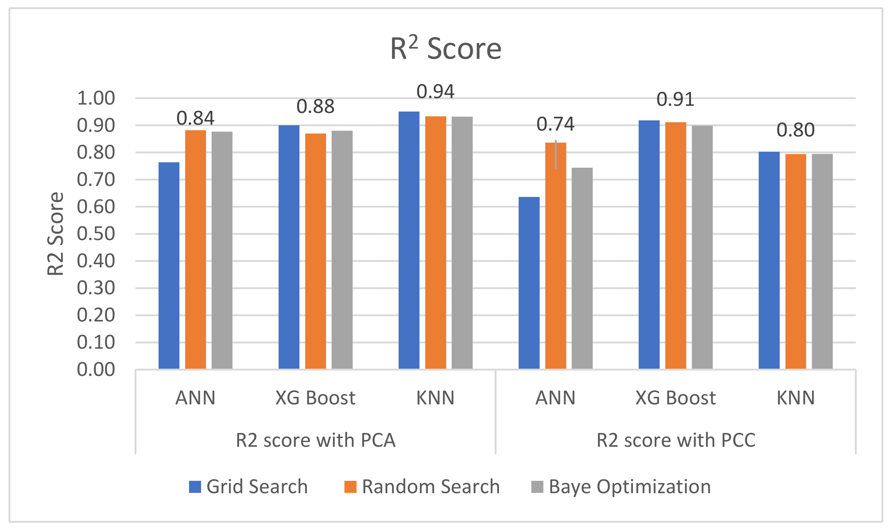
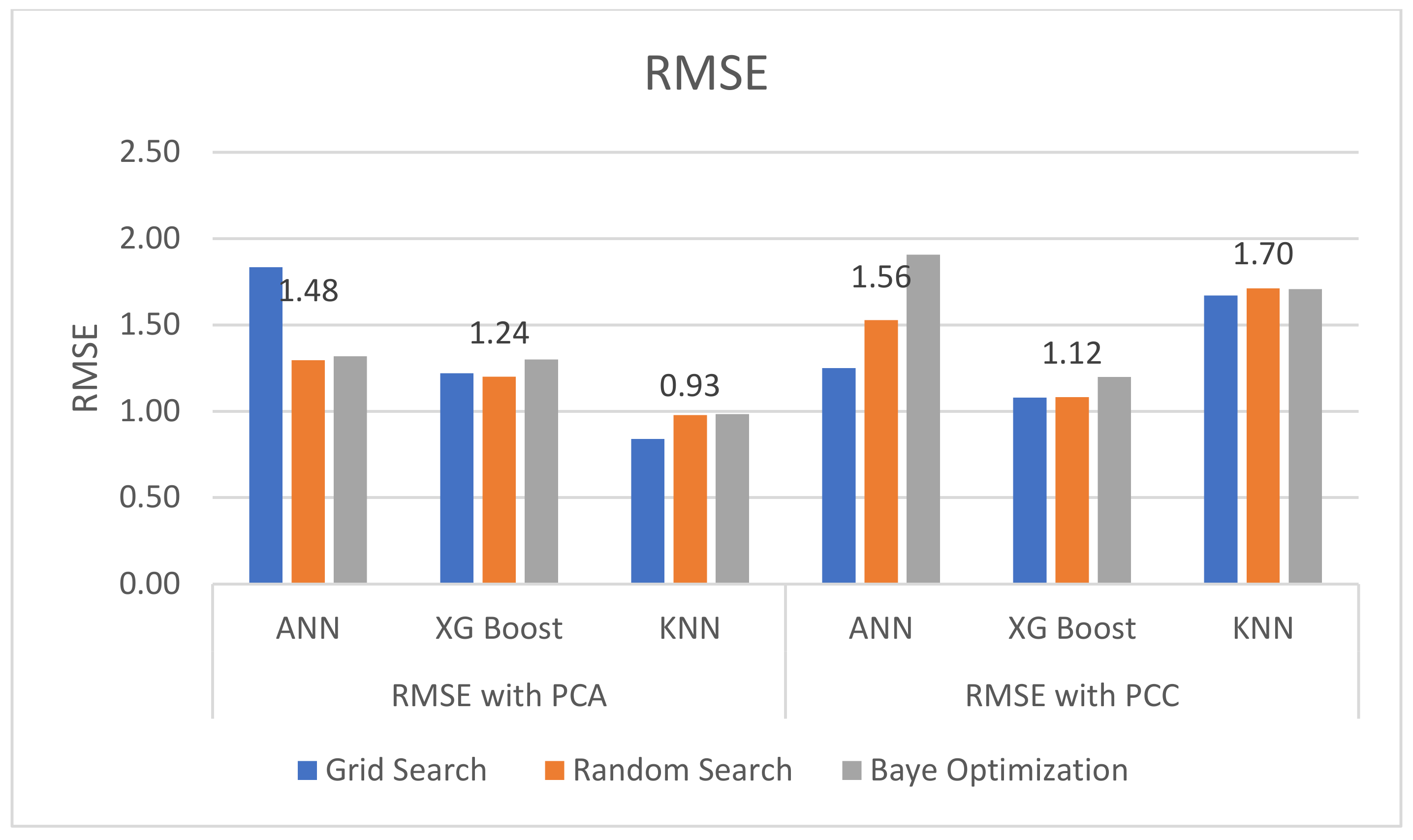
As discussed, the R² score and the RMSE are used to evaluate and compare the performance of each machine learning algorithm applied in this paper. The average R² score and RMSE are shown on top of each algorithm in Figure 16 and Figure 17, respectively. Notice that similar approaches (e.g., [56]) where error estimation and accuracy of machine learning methodologies have been performed on real datasets in different systems (e.g., vessels), or similar approaches with different Faults indicators, have been performed on the SCADA data of wind farms (e.g., [57]).

The results obtained when PCA is used as the feature selection method show a more promising result, with a lower average RMSE and a higher R² score compared to when PCC is used as the feature selection method, as shown in Figure 16. In Figure 16 and Figure 17, a grid search provided the highest RMSE and the lowest R² score when either PCA or PCC is used for feature selection. This may be because the optimal hyperparameter is not in the selected domain range. In other words, a random search gave the lowest RMSE and R² score as the optimal hyperparameter is selected randomly from a given range and the result showing the best RMSE and R² score will be chosen. The KNN model delivered the best result with the lowest RMSE, 0.84, and the highest R² score, 0.95, as shown in Figure 15 and Figure 16, with n_neighbors = 13, weights = ‘distance’ and metric=‘manhattan’.

3.4. Computational Time

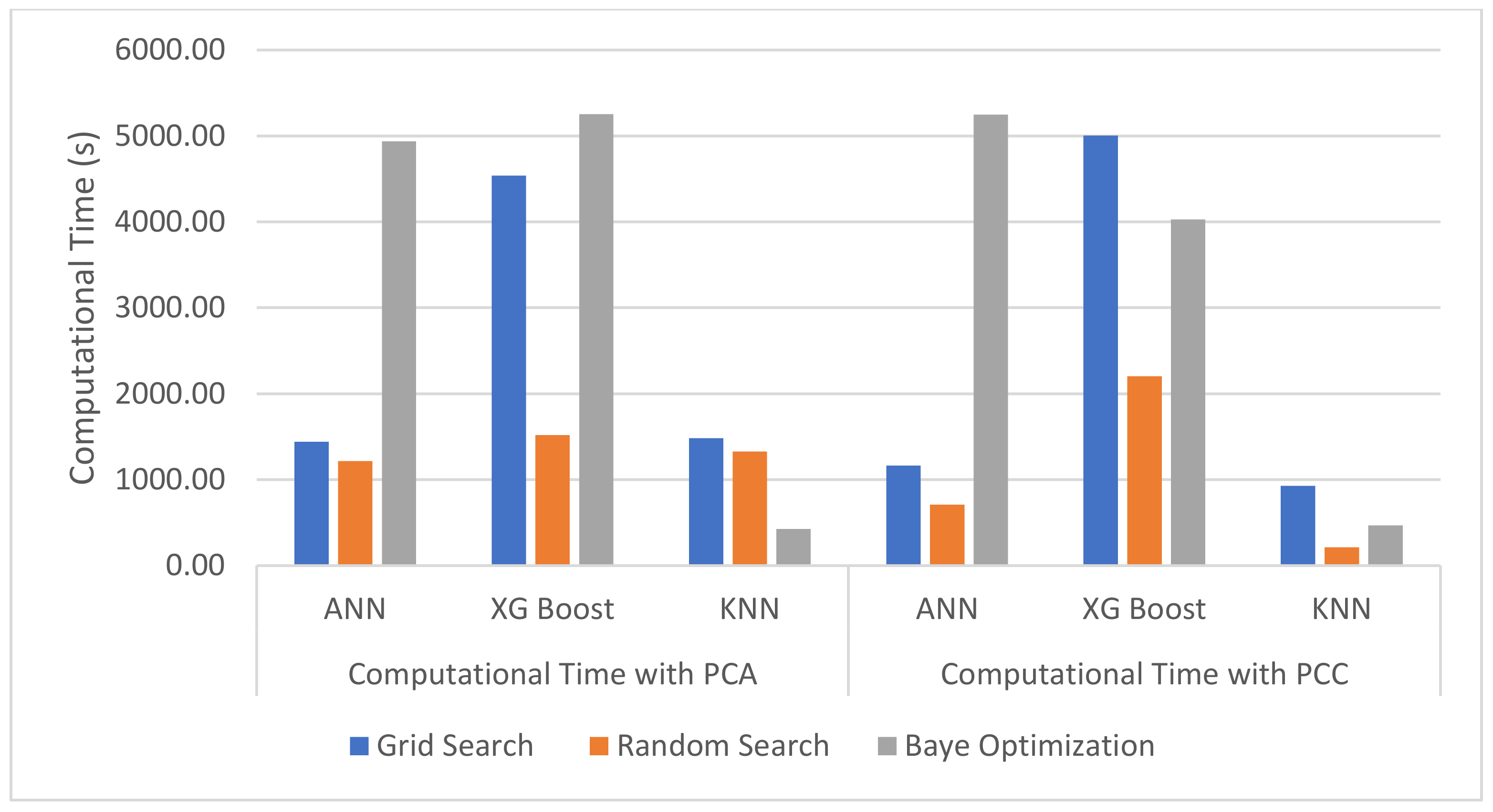
As shown in Figure 18, XGBoost had the longest computational time because XGBoost has multiple hyperparameters for optimization. KNN with a bagging regressor had a relatively lower computational time. Comparing between hyperparameter optimization methods, the random search method took the shortest computational time as the random search selected the hyperparameters in random order so as to achieve the best result as it could. The grid search and Bayesian Optimization took a longer computation time. A grid search is required to run through all the given values in each of the hyperparameters, so the greater the number of hyperparameters, the longer it takes, and this could require more computational resources. In this study, Bayesian Optimization exceeded the time set in this study and this may be due to the computational memory in the laptop.

3.5. Predicted Outcome

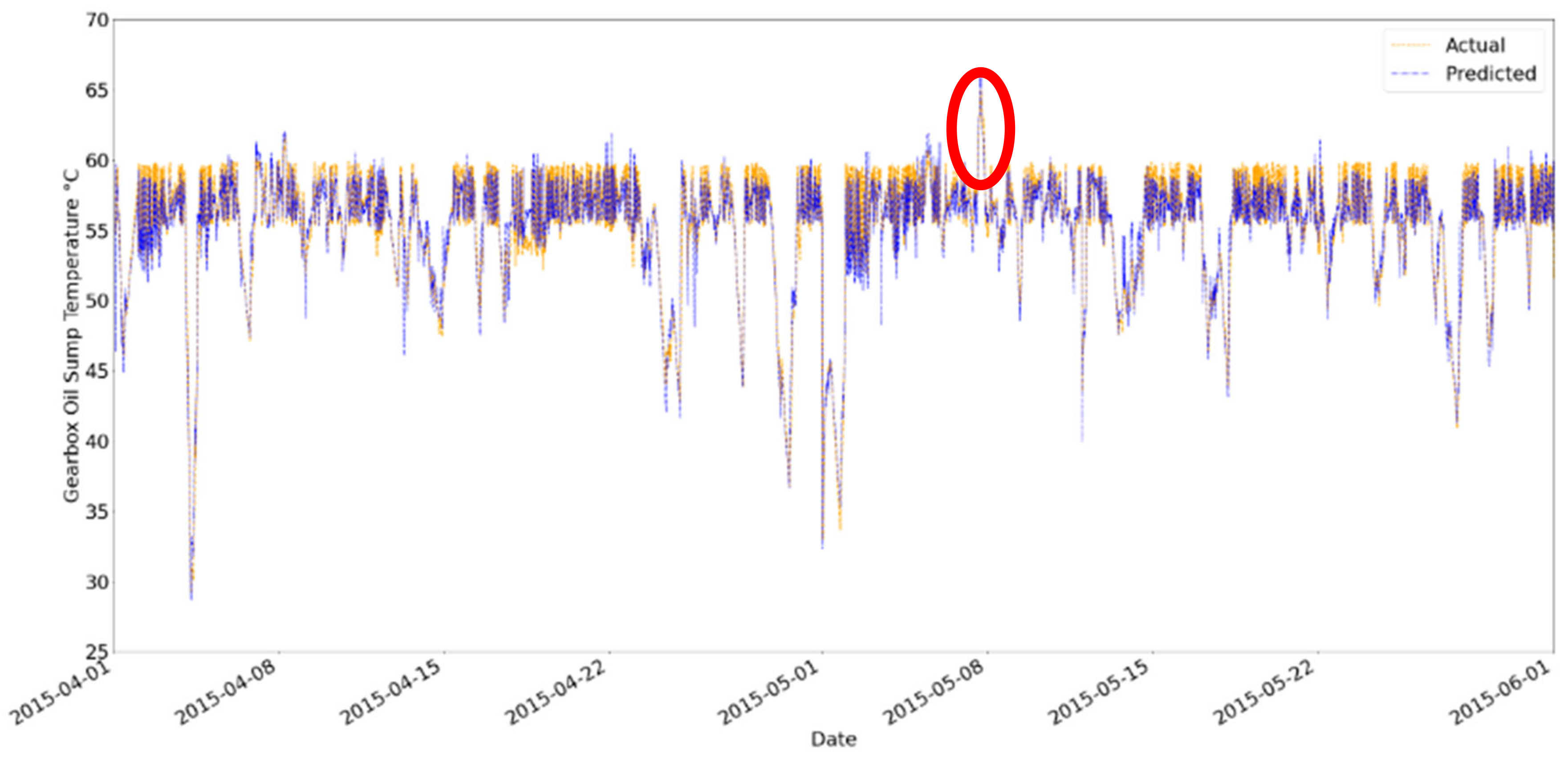
The predicted gearbox oil sump temperature is plotted against the actual gearbox oil sump temperature in Figure 19. A total of two spikes occurred as marked in the red circles. The first spike occurred on approximately 8 May 2015 and reached 65 °C, as shown in Figure 20. The second spike occurred on approximately 21 November 2016 and reached 65 °C, as shown in Figure 21. The temperature then reached approximately 30 °C on 27 November 2016 and we speculated that WT R80790 went down for maintenance during this period as the oil sump temperature reached room temperature. Next, the EWMA chart was used to determine if the trained model provides any early signals before the occurrence of these spikes.

3.6. The EMWA Chart, the First-Level Alarm and the Second-Level Alarm

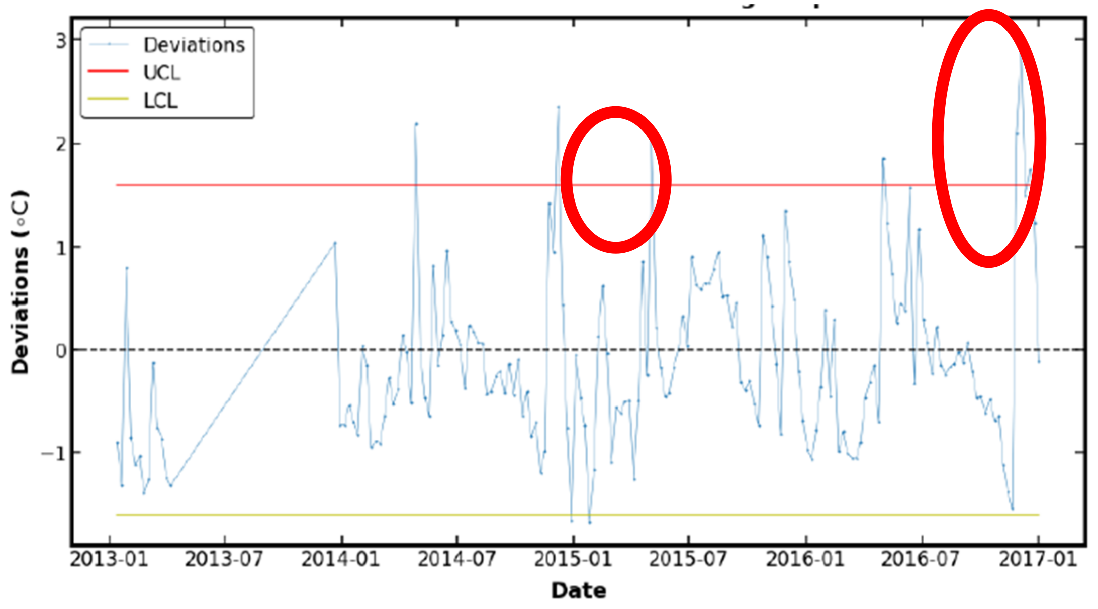
In Figure 22, the first chart is the EWMA chart for gearbox oil sump temperature deviation in R80790. The second and third charts are the first-level alarm (A1) in purple and the second-level alarm (A2) in red, respectively. A cross reference was taken from a study as mentioned in the methodology [40]. The EWMA chart for generator bearing temperature deviation in R80790 is shown in Figure 23. The study stated that WT R80790 was not in operation from 12 March 2013 to 28 December 2013.

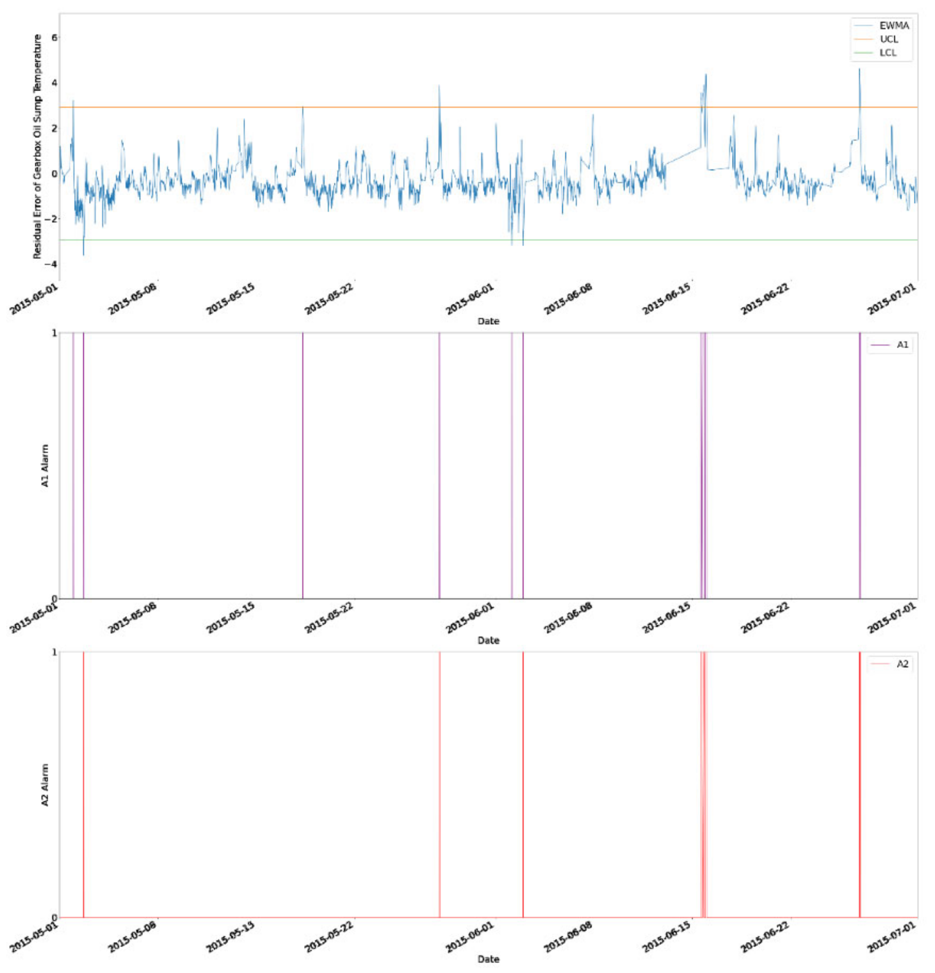
The first spike occurred on approximately 8 May 2015 and reached 65 °C, as shown in Figure 20. From Figure 24, there were two A2 alarms triggered on approximately 30 May 2015 and 2 June 2015. It was observed that the residual of generator bearing temperature deviation was over the upper control limit and lower than the lower control limit as well during this period, as shown in Figure 23. After the alarms were triggered, the gearbox oil sump temperature (GOST) reached approximately 30 and 35 °C on 15 June 2015 and 17 June 2015, respectively, where we speculated that WT R80790 underwent maintenance during this period of time. The A2 alarms were triggered approximately 15 days in advance before the maintenance action took place. The early repair action could have been performed 15 days in advance and this may lead to a shorter downtime of WT and lower maintenance cost. This would help the operator to prepare a maintenance plan in advance.

The second spike occurred on 27 November 2016, as shown in Figure 21. From the EWMA chart, the first A2 alarm and the second alarm was triggered on 25 November 2016 and 27 November 2016, respectively, as presented in Figure 25. The actual GOST reached 30 °C on 27 November 2016 and 25 °C on 21 December 2016. Further, the actual GOST also fluctuated between 25 and 30 °C from 31 December 2016 to 1 January 2017. Hence, we speculated that WT R80790 underwent maintenance during this period. The early alarm provided a warning at least 4 weeks in advance. Preventive action from major failure could thus have been taken 4 weeks in advance and this could reduce the overall O&M cost and improve the performance of the WT.

This study suggested that kNN with a bagging regressor trained model can be used for fault diagnosis in wind turbines with PCA as the feature selection method and a grid search to find the optimal hyperparameters. Furthermore, this method took the shortest computational time. However, the kNN with a bagging regressor model could be improved by training in hybrid with a Support Vector Machine as a study has shown that this could improve the performance of a kNN–SVM hybrid model [58]. The kNN–SVM hybrid model was shown to be efficient in terms of the recognition rate in this study. Further, a long short-term memory (LSTM) network could be applied in this study as well because LSTM networks can train the model by using a back-propagation tool that can be used to improve the trained model. A back-propagation tool will apply the partial derivative to determine errors at the hidden layers and input layers and update the weightage of the input for the next prediction outcome. In the future, a kNN–SVM hybrid model and a LSTM network could be applied to recognize early fault alarm in WTs.

4. Conclusions

This study evaluated the performance of two feature selection methods, namely PCA and PCC, and three different hyperparameter optimization methods, namely a grid search, a random search and Bayesian optimization, and also compared the accuracy of three different machine learning algorithms on fault diagnosis on WTs.

Overall, PCA gave a better result in terms of R² score and the RMSE compared with PCC. The number of features reduced by using PCA is greater compared with using PCC. Therefore, this may cause overfitting of the trained model as the dataset was too large. Further, Bayesian optimization takes the longest computational time compared with the other two hyperparameter optimization methods. In this study, a grid search was proposed to give the best outcome, but the grid search required high computational memory as it ran through one after another hyperparameter and stored the results for comparison. Therefore, hyperparameter optimization needs to be carefully selected as this could affect the CPU performance of the condition monitoring model.

KNN with a bagging regressor by using PCA as a feature selection method and a grid search for hyperparameter optimization was proposed in this study for fault diagnosis on WTs by predicting the gearbox oil sump temperature. The SCADA data from a wind turbine operator, ENGIE, were used in this study for validation. The results showed that the proposed method was managed to provide early alarm on WTs at least 4 weeks in advance by monitoring the residual error of gearbox oil sump temperature on an EWMA control chart and it used the shortest computational time. However, the proposed method was not as good as the method used in a study that applied the multivariate state estimation technique (MSET). The MSET is proven to give a lower rate of fault alarm [53]. Furthermore, a proper validation applied was not applied in this study as the validation part was performed based on the reference taken from another study because the actual maintenance report of the WT from ENGIE was not made available to the public.

In the future, the proposed kNN with a bagging regressor model can be further studied to improve its accuracy and can be used to provide fault alarm on other parts of WTs such as rotor blades or generators. KNN with a bagging regressor model could be trained in hybrid with a Support Vector Machine as studies have been performed on this hybrid model and show enhanced model performance [58]. Furthermore, it can be consolidated by hyperparameter optimization. The range of hyperparameters selected for optimization could be wider as the range here is limited due to the computational resource constraints in this study. If a wider range of hyperparameters are selected for optimization, this could further improve the performance of the trained model. Further, another parameter such as gearbox bearing temperature could be selected as the target variable for the chosen algorithm to determine the reliability of the algorithm. The artificial neural network can be further consolidated by applying Bayesian Physics-Informed Neural Networks as this neural network is more suitable to real-world nonlinear dynamic systems such as WTs.

References

- Lee, J. Global Wind Report 2022; Global Wind Energy Council: Brussels, Belgium, 2022. [Google Scholar]
- United Nation Climate Change. In Proceedings of the COP26: The Glasgow Climate Pact in United Nation Climate Change Conference UK, Glasgow, UK, 31 October–12 November 2021; United Nation Climate Change: Glasgow, UK, 2021.
- BloombergNEF. Wind-10 Predictions for 2022. 2022. Available online: https://about.bnef.com/blog/wind-10-predictions-for-2022/ (accessed on 13 September 2022).
- ClimateAction. Global Wind Operations & Maintenance Market to Double by 2025. 2017. Available online: https://www.climateaction.org/news/global-wind-operations-maintenance-market-to-double-by-2025 (accessed on 17 October 2022).
- Wang, C. Health Monitoring and Fault Diagnostics of Wind Turbines; Aalborg Universitet: Aalborg, Denmark, 2016. [Google Scholar] [CrossRef]
- Leahy, K.; Lily-Hu, R.; Konstantakopoulos, I.; Spanos, C.; Agogino, A. Diagnosing wind turbine faults using machine learning techniques applied to operational data. In Proceedings of the 2016 IEEE International Conference on Prognostics and Health Management (ICPHM), Ottawa, ON, Canada, 22–26 June 2016; IEEE: Piscataway, NJ, USA, 2016. [Google Scholar]
- Kohavi, R.; Provost, F. Glossary of terms. Mach. Learn. 1998, 30, 271–274. [Google Scholar]
- Education, I.C. Machine Learning 2020. Available online: https://www.ibm.com/cloud/learn/machine-learning (accessed on 13 September 2022).
- Alpaydin, E. Introduction to Machine Learning 2010; Massachusetts Institute of Technology Press: Cambridge, MA, USA; London, UK, 2010. [Google Scholar]
- TensorFlow. Available online: https://www.tensorflow.org/ (accessed on 13 September 2022).
- PyTorch. Available online: https://pytorch.org/ (accessed on 13 September 2022).
- Smiti, A. When machine learning meets medical world: Current status and future challenges. Comput. Sci. Rev. 2020, 37, 100280. [Google Scholar] [CrossRef]
- Abdella, G.M.; Kucukvar, M.; Onat, N.C.; Al-Yafay, H.M.; Bulak, M.E. Sustainability assessment and modeling based on supervised machine learning techniques: The case for food consumption. J. Clean. Prod. 2020, 251, 119661. [Google Scholar] [CrossRef]
- Xu, Y.; Zhou, Y.; Sekula, P.; Ding, L. Machine learning in construction: From shallow to deep learning. Dev. Built Environ. 2021, 6, 100045. [Google Scholar] [CrossRef]
- Salcedo-Sanz, S.; Cornejo-Bueno, L.; Prieto, L.; Paredes, D.; García-Herrera, R. Feature selection in machine learning prediction systems for renewable energy applications. Renew. Sustain. Energy Rev. 2018, 90, 728–741. [Google Scholar] [CrossRef]
- Orozco, R.; Sheng, S.; Phillips, C. Diagnostic models for wind turbine gearbox components using scada time series data. In Proceedings of the 2018 IEEE International Conference on Prognostics and Health Management (ICPHM), Seattle, WA, USA 11–13 June 2018. IEEE: Piscataway, NJ, USA, 2018. [Google Scholar]
- Rashid, H.; Batunlu, C. Anomaly Detection of Wind Turbine Gearbox based on SCADA Temperature Data using Machine Learning. Renew. Energy 2021, 3, 33. [Google Scholar]
- ENGIE. OPENdata; ENGIE: La Défense, France; Available online: https://opendata-renewables.engie.com/explore/ (accessed on 3 January 2022).
- IEC 61400-1; Commission, I.E. Wind Turbines-Part 1: Design Requirement. IEC: London, UK, 2005.
- Zaher, A.; McArthur, S.; Infield, D.; Patel, Y. Online wind turbine fault detection through automated SCADA data analysis. Wind. Energy 2009, 12, 574–593. [Google Scholar] [CrossRef]
- Yang, W.; Court, R.; Jiang, J. Wind turbine condition monitoring by the approach of SCADA data analysis. Renew. Energy 2013, 53, 365–376. [Google Scholar] [CrossRef]
- Kanungo, T.; Mount, D.M.; Netanyahu, N.S.; Piatko, C.D.; Silverman, R.; Wu, A.Y. An efficient k-means clustering algorithm: Analysis and implementation. IEEE Trans. Pattern Anal. Mach. Intell. 2002, 24, 881–892. [Google Scholar] [CrossRef]
- Brusco, M.J.; Steinley, D. A comparison of heuristic procedures for minimum within-cluster sums of squares partitioning. Psychometrika 2007, 72, 583–600. [Google Scholar] [CrossRef]
- De Maesschalck, R.; Jouan-Rimbaud, D.; Massart, D.L. The mahalanobis distance. Chemom. Intell. Lab. Syst. 2000, 50, 1–18. [Google Scholar] [CrossRef]
- Lee, J.; Wang, W.; Harrou, F.; Sun, Y. Wind power prediction using ensemble learning-based models. IEEE Access 2020, 8, 61517–61527. [Google Scholar] [CrossRef]
- Liu, Y.; Mu, Y.; Chen, K.; Li, Y.; Guo, J. Daily activity feature selection in smart homes based on pearson correlation coefficient. Neural Process. Lett. 2020, 51, 1771–1787. [Google Scholar] [CrossRef]
- Midi, H.; Sarkar, S.; Rana, S. Collinearity diagnostics of binary logistic regression model. J. Interdiscip. Math. 2010, 13, 253–267. [Google Scholar] [CrossRef]
- Calkins, K.G. Applied Statistics-Lesson 5. Correlation Coefficients 2005. Available online: https://www.andrews.edu/~calkins/math/edrm611/edrm05.htm#:~:text=Correlation%20coefficients%20whose%20magnitude%20are,can%20be%20considered%20highly%20correlated (accessed on 10 October 2022).
- Granato, D.; Santos, J.S.; Escher, G.B.; Ferreira, B.L.; Maggio, R.M. Use of principal component analysis (PCA) and hierarchical cluster analysis (HCA) for multivariate association between bioactive compounds and functional properties in foods: A critical perspective. Trends Food Sci. Technol. 2018, 72, 83–90. [Google Scholar] [CrossRef]
- Feurer, M.; Hutter, F. Hyperparameter Optimization, in Automated Machine Learning; Springer: Cham, Switzerland, 2019; pp. 3–33. [Google Scholar]
- Bhat, P.C.; Prosper, H.B.; Sekmen, S.; Stewart, C. Optimizing event selection with the random grid search. Comput. Phys. Commun. 2018, 228, 245–257. [Google Scholar] [CrossRef] [Green Version]
- Eggensperger, K.; Feurer, M.; Hutter, F.; Bergstra, J.; Snoek, J.; Hoos, H.; Leyton-Brown, K. Towards an empirical foundation for assessing bayesian optimization of hyperparameters. In Proceedings of the NIPS workshop on Bayesian Optimization in Theory and Practice, Lake Tahoe, NV, USA, 10 December 2013. [Google Scholar]
- Scikit-Learn. Available online: https://scikit-learn.org/stable/ (accessed on 28 September 2022).
- Bishop, C.M.; Nasrabadi, N.M. Pattern Recognition and Machine Learning; Springer: Berlin/Heidelberg, Germany, 2006; Volume 4. [Google Scholar]
- Farahnakian, F.; Pahikkala, T.; Liljeberg, P.; Plosila, J. Energy aware consolidation algorithm based on k-nearest neighbor regression for cloud data centers. In Proceedings of the 2013 IEEE/ACM 6th International Conference on Utility and Cloud Computing, Dresden, Germany, 9–12 December 2013; IEEE: Piscataway, NJ, USA, 2013. [Google Scholar]
- Breiman, L. Bagging predictors. Mach. Learn. 1996, 24, 123–140. [Google Scholar] [CrossRef] [Green Version]
- Kovačević, M.; Ivanišević, N.; Petronijević, P.; Despotović, V. Construction cost estimation of reinforced and prestressed concrete bridges using machine learning. Građevinar 2021, 73, 1–13. [Google Scholar]
- Chen, T.; He, T.; Benesty, M.; Khotilovich, V.; Tang, Y.; Cho, H.; Chen, K. Xgboost: Extreme Gradient Boosting. R Package Version 0.4-2. 2015, Volume 1, pp. 1–4. Available online: https://cran.microsoft.com/snapshot/2017-12-11/web/packages/xgboost/vignettes/xgboost.pdf (accessed on 28 October 2022).
- Friedman, J.H. Greedy function approximation: A gradient boosting machine. Ann. Stat. 2001, 29, 1189–1232. [Google Scholar] [CrossRef]
- Udo, W.; Muhammad, Y. Data-driven predictive maintenance of wind turbine based on SCADA data. IEEE Access 2021, 9, 162370–162388. [Google Scholar] [CrossRef]
- Thorn, J. What is Boosting in Machine Learning? 2020. Available online: https://towardsdatascience.com/what-is-boosting-in-machine-learning-2244aa196682 (accessed on 28 September 2022).
- Ogunleye, A.; Wang, Q.-G. XGBoost model for chronic kidney disease diagnosis. IEEE/ACM Trans. Comput. Biol. Bioinform. 2019, 17, 2131–2140. [Google Scholar] [CrossRef] [PubMed]
- Education, I.C. Gradient Descent. 2020. Available online: https://www.ibm.com/cloud/learn/gradient-descent#:~:text=Gradient%20descent%20is%20an%20optimization,each%20iteration%20of%20parameter%20updates (accessed on 28 September 2022).
- Kwiatkowski, R. Gradient Descent Algorithm-A Deep Dive. 2021. Available online: https://towardsdatascience.com/gradient-descent-algorithm-a-deep-dive-cf04e8115f21 (accessed on 28 September 2022).
- Haykin, S. Neural Networks and Learning Machines, 3/E; Pearson Education India: Chennai, India, 2009. [Google Scholar]
- Dertat, A. Applied Deep Learning-Part 1: Artificial Neural Networks. 2017. Available online: https://towardsdatascience.com/applied-deep-learning-part-1-artificial-neural-networks-d7834f67a4f6 (accessed on 16 October 2022).
- Gardner, M.W.; Dorling, S. Artificial neural networks (the multilayer perceptron)—A review of applications in the atmospheric sciences. Atmos. Environ. 1998, 32, 2627–2636. [Google Scholar] [CrossRef]
- Dennis, S. Introduction to Neural Network. 1997. Available online: http://users.csc.calpoly.edu/~dsun09/data401/handouts/neural_networks_slides.pdf (accessed on 29 October 2022).
- Stetco, A.; Dinmohammadi, F.; Zhao, X.; Robu, V.; Flynn, D.; Barnes, M.; Keane, J.; Nenadic, G. Machine learning methods for wind turbine condition monitoring: A review. Renew. Energy 2019, 133, 620–635. [Google Scholar] [CrossRef]
- Kong, Z.; Tang, B.; Deng, L.; Liu, W.; Han, Y. Condition monitoring of wind turbines based on spatio-temporal fusion of SCADA data by convolutional neural networks and gated recurrent units. Renew. Energy 2020, 146, 760–768. [Google Scholar] [CrossRef]
- Perry, M.B. The exponentially weighted moving average. In Wiley Encyclopedia of Operations Research and Management Science; Wiley Online Library: New York, NY, USA, 2010. [Google Scholar]
- Li, H.; Deng, J.; Yuan, S.; Feng, P.; Arachchige, D.D.K. Monitoring and Identifying Wind Turbine Generator Bearing Faults Using Deep Belief Network and EWMA Control Charts. Front. Energy Res. 2021, 9, 799039. [Google Scholar] [CrossRef]
- Wang, Z.; Liu, C.; Yan, F. Condition monitoring of wind turbine based on incremental learning and multivariate state estimation technique. Renew. Energy 2022, 184, 343–360. [Google Scholar] [CrossRef]
- Verbruggen, T. Wind Turbine Operation & Maintenance Based on Condition Monitoring WT-Ω; Final Report; US Department of Energy: Washington, DC, USA, 2003.
- Xiang, L.; Yang, X.; Hu, A.; Su, H.; Wang, P. Condition monitoring and anomaly detection of wind turbine based on cascaded and bidirectional deep learning networks. Appl. Energy 2022, 305, 117925. [Google Scholar] [CrossRef]
- Theodoropoulos, P.; Spandonidis, C.C.; Themelis, N.; Giordamlis, C.; Fassois, S. Evaluation of Different Deep-Learning Models for the Prediction of a Ship’s Propulsion Power. J. Mar. Sci. Eng. 2021, 9, 116. [Google Scholar] [CrossRef]
- Encalada-Dávila, Á.; Puruncajas, B.; Tutivén, C.; Vidal, Y. Wind turbine main bearing fault prognosis based solely on SCADA data. Sensors 2021, 21, 2228. [Google Scholar] [CrossRef]
- Zanchettin, C.; Bezerra, B.L.D.; Azevedo, W.W. A KNN-SVM hybrid model for cursive handwriting recognition. In Proceedings of the 2012 International Joint Conference on Neural Networks (IJCNN), San Diego, CA, USA, 17–21 June 2012; IEEE: Piscataway, NJ, USA, 2012. [Google Scholar]
Figure 1.
Cost Distribution of an Offshore Wind Turbine [5].
Figure 2.
Downtime Caused by WTs in the Egmondaan Zee Wind Farm in the Netherlands in 2008 and 2009 [5].
Figure 3.
Typical WT Power vs. Wind Speed Curve.
Figure 4.
K-Means Elbow.
Figure 5.
Scree Plot for PCA.
Figure 6.
Elbow Curve for kNN Regressor.
Figure 7.
Bootstraps in Regression Tree Ensembles [37].
Figure 8.
Boosting in Machine Learning [41].
Figure 9.
Multilayer Perceptron System [46].
Figure 10.
Transfer Function [48].
Figure 11.
Schematic of Flow Chart of Proposed Condition Monitoring Framework.
Figure 12.
K-Means Clustering of Each WT.
Figure 13.
Power vs. Wind Speed Curve of Each WT.
Figure 14.
The Pearson Correlation Coefficient Heatmap.
Figure 15.
PC1 vs. PC2.
Figure 16.
R2 Scores Obtained from Each Model with PCA and PCC.
Figure 17.
RMSEs Obtained from Each Model with PCA and PCC.
Figure 18.
Computation Time for Each Hyperparameter Optimization Method in PCA and PCC.
Figure 19.
Predicted and Actual Gearbox Oil Sump Temperatures in R80790 WT vs. Date [January 2016 to January 2017].
Figure 20.
Predicted and Actual Gearbox Oil Sump Temperatures in R80790 WT vs. Date [April 2015 to June 2015].
Figure 21.
Predicted and Actual Gearbox Oil Sump Temperatures in R80790 WT vs. Date [November 2016 to December 2016].
Figure 22.
EWMA Chart with A1 and A2 Alarms.
Figure 23.
EWMA Chart for Generator Bearing Temperature Deviation in R80790.
Figure 24.
EWMA Chart with A1 and A2 Alarms from May 2015 to July 2015.
Figure 25.
EWMA Chart with A1 and A2 Alarms from November 2016 to January 2017.