Article

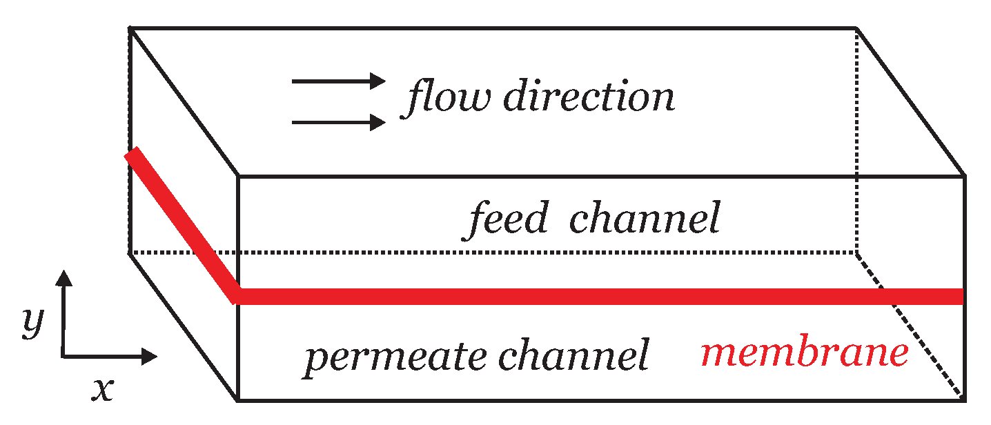
Mass Transport in Membrane Systems: Flow Regime Identification by Fourier Analysis

1
Department of Mathematics and Statistics, University of Wyoming, 1000 East University Avenue, Laramie, WY 82071, USA
2
Department of Biomedical Engineering, Johns Hopkins University, 3400 N. Charles St., Baltimore, MD 21218, USA
3
Department of Civil & Architectural Engineering, University of Wyoming, 1000 East University Avenue, Laramie, WY 82071, USA
*
Author to whom correspondence should be addressed.
Fluids 2022, 7(12), 369; https://doi.org/10.3390/fluids7120369
Submission received: 10 October 2022 / Revised: 9 November 2022 / Accepted: 11 November 2022 / Published: 30 November 2022
(This article belongs to the Special Issue Recent Advances in Fluid Mechanics: Feature Papers, 2022)

Abstract

:
The numerical calculation of local mass distributions in membrane systems by computational fluid dynamics (CFD) offers indispensable benefits. However, the concept to calculate such distributions in response to separate variations of operation conditions (OCs) makes it difficult to address overall, flow-physics-related questions, which require the consideration of the collective interaction of OCs. It is shown that such understanding-related relationships can be obtained by the analytical solution of the advection–diffusion equation considered. A Fourier series model (FSM) is presented, which provides exact solutions of an advection–diffusion equation for a wide range of OCs. On this basis, a new zeroth-order model is developed, which is very simple and as accurate as the complete FSM for all conditions of practical relevance. Advection-dominated blocked and diffusion-dominated unblocked flow regimes are identified (depending on a Péclet number which compares the flow geometry with a length scale imposed by the flow), which implies relevant requirements for the use of lab results for pilot- and full-scale applications. Analyses reveal the equivalence of variations of OCs, which offers a variety of options to accomplish desired flow regime changes.

1. Introduction

Computational studies of membrane systems as illustrated in Figure 1 enable very valuable insight into the effectiveness of performance measures, e.g., with respect to concentration polarization and fouling [1,2,3,4,5,6,7,8,9,10,11], as well as evaluating flow unsteadiness induced by different spacer configurations [12,13,14,15,16,17,18,19,20,21,22,23,24,25,26,27,28]. Such computational insights are invaluable given the experimental challenges associated with directly quantifying such phenomena. In one recent study, Liang et al. [29] used two-dimensional (2D) computational fluid dynamics (CFD; the use of this term refers here to the numerical solution of partial differential equations) simulations to resolve the roles played by bulk flow and slip velocities at a membrane surface for generating shear forces at the membrane surface. From this work, it was determined that the origin of shear induction was less important when compared with the resonant frequency of the perturbations themselves for increasing flux through the disruption of foulant and concentration polarization boundary layers. Similarly valuable insights into improving the hydrodynamic conditions within spiral wound membrane elements were made by Foo et al. [30]. Using CFD, these researchers identified optimum spacer geometries for enhancing water flux (up to a 40% flux enhancement) through a membrane through maximizing unsteady-state shear forces at a membrane surface. Reaching this outcome, as is the case in other similar studies, required computationally intensive evaluations of the hydrodynamic environments within the membrane flow channels. Regardless of the complexities involved, the impacts that such studies have on improving the performance and energy efficiency of membrane processes is obvious.
Despite the indispensable benefits of CFD, the use of such numerical investigation methods is non-trivial, time-consuming, dependent on the availability of numerical codes, and affected by the numerical schemes applied [31,32,33,34,35,36,37,38,39]. For example, the influence of Péclet numbers (see Equation (6)) has consequences for the equation type considered and the numerical solution of these equations. The equation shows a parabolic (hyperbolic) behavior if the Péclet number is small (large). The numerical solution of such equations becomes increasingly difficult as the Péclet number increases due to the onset of spurious oscillations or excessive numerical damping if standard finite difference or finite element formulations are used [40]. A particular problem is the usual application of Reynolds-averaged Navier–Stokes (RANS) equations. If spacers are involved, separated flow will appear (recirculation zones), and RANS equations are known to not have the capability to deal with such flow features (the latter requires the use of rather sophisticated, partially resolving flow simulation methods [41,42,43,44,45,46,47,48]). On top of knowledge about detailed mass distributions in membrane systems for specific operation conditions OCs provided by CFD, knowledge of specific flow regimes (which may have desired or undesired characteristics) is very helpful for the membrane system design process. Diffusion–advection processes are characterized by diffusion-dominated and advection-dominated flow regimes, which are separated by corresponding Péclet numbers [40,49]: when this number is small (large), then diffusion (advection) dominates. However, there is a large variety of Péclet numbers that can be considered [50], there are often fuzzy criteria for characterizing different flow regimes (such as Péclet numbers larger or smaller than unity), and the practical consequences of such regime separations are not always obvious. So, there are questions regarding the membrane system design (see also Figure 2):
Q1.
What determines the existence of qualitatively different mass transport regimes? Which interplay of geometry and OCs is implied, which matters to upscaling?
Q2.
How is it possible to accomplish desired flow regime changes by equivalent variations of OCs?
Q3.
For different flow regimes, how is it possible to understand the overall mass transport through membranes and characteristic mass distribution features?
The CFD approach often provides an inappropriate basis to address these questions: separate parameter variations hardly allow conclusions about collective parameter effects.
Figure 2. An illustration of the flow configuration considered and flow physics questions addressed (in blue). Operation condition parameters are given in red. Partial derivatives ( c x and c y ) are indicated here by subscripts.
Fluids 07 00369 g002
In addition to CFD, the use of analytical simulation methods is beneficial because of several reasons. Their use hardly depends on the availability of codes. They are by orders of magnitude more efficient than the numerical integration of partial differential equations in time because of the independence of discretizations and the need to honor numerical stability criteria under significant model parameter variations. Such analytical simulation methods can be used for the verification of numerical solvers because they provide exact results (i.e., independent evidence is not needed to support them). However, first of all, the availability of such models offers the chance to address questions about basic mass transport mechanisms, e.g., regarding the questions Q1–Q3 presented above.
One question related to the use of analytical simulation methods is about their required complexity and simplicity of using them. For the case considered, analytical simulation methods are given by Fourier series representations, there is the question of whether the complexity of such Fourier series representations can be significantly reduced to enhance the clarity of conclusions. Another question related to analytical simulation methods is that their development requires the neglect of effects of spacers, which modify basic flow characteristics implied by geometry, inflow and boundary conditions. The specification of spacer effects on the basic flow configuration varies in the literature [30,51,52]. There are indications that spacers can produce higher fluxes of about 30–40% compared with cases without spacers [30,51,52]. This means analytical simulation methods can be expected to provide valuable guidelines for the characterization of basic flow features, even under conditions where spacers and other effects (flow unsteadiness) are involved. Thus, there are questions in addition to Q1–Q3 considered above:
Q4.
What is the most simple analytical model which still enables accurate calculations equivalent to complete Fourier series solutions?
Q5.
Given the required approximate representation of the flow field, which arguments support the use of analytical simulation methods under more complex flow conditions?
Analytical solutions obtained by Laplace transforms were presented for a variety of problems, for example, in regard to turbulent dispersion of air pollution [53] and diffusion of oxygen into the blood [54], but no corresponding solutions were presented in regard to membrane systems. The corresponding value of analytical simulation methods is demonstrated here by addressing the questions Q1–Q5 presented above. Fourier analysis is applied for the derivation of analytical results, which offers (via the analysis of eigenvalue regimes) essential new insight. The model development is presented in Section 2 in conjunction with the consideration of questions about the model evaluation and computational aspects. Model applications are reported in Section 3 by focusing on the influence of OCs on species concentration distributions. Section 4 deals with conclusions about the questions considered.

2. Model Development

2.1. Equation Considered

Incompressible flow and a 2D domain are considered, see the illustration in Figure 2. The velocity field is approximated by assuming constant velocities U and V in the x and y directions, which is a requirement to obtain analytical solutions. The suitability of this assumption is considered in Section 4, conclusion #5, in conjunction with mass transport properties. A mixture (e.g., an oil-in-water emulsion) of a continuous phase (e.g., water) and a dispersed phase (e.g., oil at low concentrations) is considered. The solutions presented below are not specific to oil-in-water emulsions, they can be applied to many other systems. According to refs. [7,10,55], the dispersed phase transport equations in the feed/permeate region and membrane region (see Figure 1), respectively, read
c t + U c x + V c y = D M 2 c x 2 + 2 c y 2 , ϵ p c t + U c x + V c y = D c 2 c x 2 + 2 c y 2 .
Here, c refers to the dispersed phase concentration, t is time, D M refers to the molecular diffusion (of oil in water), D c refers to the capillary diffusion, and ϵ p is the membrane porosity. The constant diffusivities D M and D c are considered in consistency with the consideration of constant velocities U and V. Diffusion in x direction (which is sometimes neglected) is included. No attempt is made to differentiate between the velocities U and V involved in Equation (1) because these equations are covered by one equation in the following, in particular, the advection–diffusion equation of the membrane region,
c t + U ^ c x + V ^ c y = D c ^ 2 c x 2 + 2 c y 2 .
Here, U ^ = U / ϵ p , V ^ = V / ϵ p , and D c ^ = D c / ϵ p are introduced. The solution obtained can be easily applied as a solution to the feed/permeate region equation by a corresponding adjustment of model parameters (by setting ϵ p = 1 and replacing D c by D M ). The domain considered is 0 x x 2 and y 1 y y 2 ; see the illustration in Figure 2. By involving imposed functions g ( x , y ) and f ( y ) , the initial distribution and x boundary conditions (BCs) at x = x 1 = 0 and x = x 2 are given by
c ( x , y , 0 ) = g ( x , y ) , c ( 0 , y , t ) = f ( y ) , c x ( x 2 , y , t ) = 0 .
The latter condition applies to the case that diffusion in x direction is included. The y BCs at y = y 1 and y = y 2 are given by
c y ( x , y 1 , t ) = 0 , c ( x , y 2 , t ) V ^ / δ + D c ^ c y ( x , y 2 , t ) = 0 .
The y BCs modify a constant mass transfer (zero gradient) along y by the condition at y 2 , which leads to an accumulation of the dispersed phase in the membrane region; see the discussion in the beginning of Section 3. The parameter δ introduced here enables variations of the mass transfer at y 2 ; Equation (A2) in the Appendix A shows that 2 / δ represents the standardized membrane permeability. The introduction of δ is relevant to the identification of the critical Péclet number P e c = 4 / ( 2 + δ ) in Section 3.1. The measurement of δ is addressed in Section 3.2. Implications of these BCs may be well seen in figures below (although the effects may be small, see the distributions along x ).
An important property of the solution c ( x , y , t ) is its boundedness: if the initial and boundary values of c ( x , y , t ) lie within a minimum and maximum, c m i n c c m a x , then all c ( x , y , t ) values are bounded by this range [56]. The consideration of an advection–diffusion equation for the dispersed phase is equivalent to the consideration of a stochastic particle model for this phase (a random model for the positions of oil droplets, a Brownian motion model originally applied to describe the motion of pollen grains in water) where the mass concentration represents a non-normalized probability density function (PDF) [57]: the concentration has all the properties of a PDF except that it is not normalized.
It is helpful to introduce normalized variables: x = U ^ x / ( 2 D c ^ ) , y = V ^ y / ( 2 D c ^ ) , and t = V ^ 2 t / ( 4 D c ^ ) . By using these normalized variables, Equation (2) reads
c t + 2 U 2 V 2 c x + 2 c y = U 2 V 2 2 c x 2 + 2 c y 2 .
The equations derived in the following reveal that c = c x , y y 1 , t | x 2 , Δ , δ , U / V , where Δ = y 2 y 1 . It is convenient to introduce usually applied non-dimensional numbers, the aspect ratio A, the Péclet number P e , and the Péclet number P e y in y direction,
A = x 2 y 2 y 1 , P e = U ^ x 2 D c ^ , P e y = V ^ ( y 2 y 1 ) D c ^ .
P e and P e y represent the product of corresponding Reynolds numbers ( U ^ x 2 / ν and V ^ ( y 2 y 1 ) / ν , respectively) with the Schmidt number ν / D c ^ , where ν is the kinematic viscosity. By applying the relationships
x 2 = P e / 2 , Δ = P e y / 2 , U / V = P e / ( A P e y ) ,
the solution c = c x , y y 1 , t | x 2 , Δ , δ , U / V can be written in the following way:
c = c ( x , y y 1 , t | A , P e , P e y , δ ) .
The solution c ( x , y , t ) to Equation (5) involves two ingredients, the stationary solution s ( x , y ) for infinitely large t and the transitional solution w ( x , y , t ) ,
c ( x , y , t ) = s ( x , y ) + w ( x , y , t ) .
The stationary and transitional solutions s ( x , y ) and w ( x , y , t ) , which are referred to as stationary Fourier series model (FSM) and transitional Fourier series model (FSM), are given by Equation (A3) and Equation (A17), respectively; see the explanations in the Appendix A.

2.2. Validation of the Model Implementation

The equations were implemented in an in-house code written for this application. In numerical model applications, the use of the stationary and transitional FSMs obtained ensures exact solutions to the advection–diffusion equation considered. Relatively simple analysis also shows that the use of the structures of X n ( x ) and U n ( y ) given in the Appendix A ensures the correct upper and lower y BCs and outflow BCs. However, the inflow BCs represented by the sum of Fourier series contributions in the model implementation require validation because they are affected by the numerical implementation, for example, the correct calculation of eigenvalues. This question is addressed in terms of Figure 3, which shows the concentration distribution along y / Δ for reference parameters P e y = 1 , P e = 10 2 , A = 10 3 , δ = 10 , and δ = 1 at x = 0 . The dashed lines represent the imposed profile, the colored lines arise from imitated implementation errors: the neglect of one eigenfunction contribution, and the incorrect calculation of one eigenvalue ( β 0 m or β 0 p , respectively) given by a modification by a factor of 2 or 0.5. It may be seen that such incorrect implementations have serious consequences. Both the neglect of one eigenfunction contribution or an eigenvalue modification (by a factor of 2 or 0.5) implies that the model is incapable to correctly provide the imposed profile. Therefore, checks whether concentration calculations are in consistency with imposed profiles are sufficient to conclude that the model implementation is correct. A relatively simple way to provide additional support for the correct model implementation is to ask whether the solutions obtained satisfy the boundedness of mass transport requirement. This is, e.g., not the case for the cases with implementation errors presented in Figure 3: such model results disagree with the boundedness of mass transport because concentration values below zero and above one are obtained. For all the cases presented below, it was found that the boundedness requirements were satisfied by model solutions.

2.3. Computational Cost

The computational cost of the presented method depends very much on the convergence behavior of Fourier representations involved. The stationary solution is driven by the convergence of y eigenfunctions. A scaling analysis reveals that U n ( y 2 ) ( q 1 q 2 ) P e y / n 2 at sufficiently high n, where q 1 and q 2 are positive and negative numbers of order unity (which are related to the two contributions to a n in Table A1). Correspondingly, transitional solution contributions scale with w 2 ( y 2 , 0 ) q 1 P e y / n 2 , where q 0 is a positive number of order unity. The easiest way to see these scalings is to multiply series contributions with the inverse scaling to demonstrate that series contributions do not change with n and parameter variations. Let us suppose the convergence requirement that the related Fourier series contributions need to be smaller than 10 9 . This implies the condition P e y / N 2 10 9 , i.e., N 10 4.5 P e y 1 / 2 3.2 × 10 4 P e y 1 / 2 . For usual values P e y 1 , this condition can be easily satisfied (in less than a minute). A corresponding scaling analysis of x eigenfunctions involved in the transitional solution part shows that w 1 ( x 2 , 0 ) ( 1 ) n + 1 q P e ( 1 + 2 / P e ) / n 3 , where q is a positive number of order unity. By using again a convergence criterion that corresponding Fourier series contributions need to be smaller than 10 9 , the corresponding convergence condition reads P e / N 3 10 9 for sufficiently high P e , this means N 10 3 P e 1 / 3 . For P e = ( 10 2 , 10 3 , 10 4 ) , for example, one finds N ( 4.6 × 10 3 , 10 4 , 2.2 × 10 4 ) . Such simulations take much less than a minute on a personal computer. A very essential observation is the following. In contrast to the stationary solution s ( x , y ) , the transitional solution w ( x , y , t ) = c i n w 1 ( x , t ) w 2 ( y , t ) is given by separated variations in x and y . This makes computations by orders of magnitude more efficient because a double loop over x and y eigenvalues does not appear.
Figure 3. The concentration distribution along y from y 1 (lower bound) to y 2 (upper bound) for reference parameters P e y = 1 , P e = 10 2 , A = 10 3 , and δ = 10 in (a) and δ = 1 in (b) at x = 0 (dashed lines). The red lines refer to the neglect of β 0 m or β 0 p , respectively, eigenfunction contributions. The blue and green lines refer to a modification of β 0 m or β 0 p , respectively, by the given factors (2 and 0.5).
Fluids 07 00369 g003
The computational development of the simulation method leads to four observations. (i) The computational method is computationally highly efficient: exact solutions are obtained on a personal computer in less than a minute. (ii) A specific question related to the computational cost is about the scaling of cost with model parameters such as the Péclet numbers involved ( P e and P e y ). It was shown that such model parameter variations have very minor effects on the solution convergence with respect to both the stationary and transitional solution. (iii) One key element of correct solutions is the exact iterative solution of eigenvalue equations for all parameter regimes, which represents a challenging task. An efficient algorithm for handling this question was presented here. (iv) Another key element is, in particular, the correct identification of the lowest order eigenvalues for all parameter regimes, otherwise the method simply does not work.

3. Model Application

Results using the model obtained are presented now by focusing for simplicity on the stationary solution (the transitional solution is discussed in Section 3.2)
c = c ( x , y y 1 | A , P e , P e y , δ ) .
The parameters involved are given by Equation (6). As shown in the Appendix A in the paragraph below Equation (A6), the critical parameter that separates different eigenvalue regimes is given by p = 2 / δ ( 1 + 2 / δ ) P e y / 2 (see also the illustration in Figure 4). To restrict attention, it is assumed that δ 0 . According to the BC, s ( x , y 2 ) + [ δ / 2 ] [ s / y ] ( x , y 2 ) = 0 , which implies a negative concentration gradient at y 2 ; this is equivalent to the calculation of a concentration (of oil) that has at the lower boundary y 1 a larger value than at the upper boundary y 2 . It is worth noting that the assumption δ < 0 , which implies decreasing concentration values toward the lower boundary, may well be in conflict with the boundedness of mass transport for the conditions considered because concentration values larger than unity can be obtained.

3.1. FSM: Flow Regimes and Equivalent OC

The concentration distribution at x = x 2 and y = y 1 is shown in Figure 5 for varying parameters A , P e , P e y , and δ . The most relevant observation is that p = 2 / δ ( 1 + 2 / δ ) P e y / 2 , which separates different eigenvalue regimes and also separates different concentration regimes; see Figure 5a. For p < 0 , one finds high concentration values which do not change much with δ . We refer to this case as blocked flow below. For p > 0 , one finds much lower concentration values which are, approximately, linearly controlled by δ . We refer to this case below as unblocked flow. The critical P e y for which p = 0 reads P e c = 4 / ( 2 + δ ) , which is bounded, 0 P e c 2 . Hence, p can be written p = 2 ( 1 P e y / P e c ) / δ . Here, P e y / P e c represents a normalized Péclet number. By introducing L f = P e c D c ^ / V ^ , it can be written P e y / P e c = ( y 2 y 1 ) / L f . Correspondingly, the conditions for the unblocked (blocked) flow regimes are given by
y 2 y 1 < L f ( y 2 y 1 > L f ) ,
respectively. Here, L f represents a characteristic length scale which depends only on flow properties. Equation (11) state, therefore, the requirement that the domain height has to be sufficiently small to enable unblocked flow. The relationship between unblocked/blocked flow and diffusion/advection-dominated flow regimes can be seen as follows. In unblocked flow, the diffusion dominates: molecular transport governs this regime basically unaffected by the directional influence of advection. It is, therefore, very natural to identify the unblocked (blocked) flow regimes as diffusion (advection)-dominated flow. According to p = 2 ( 1 P e y / P e c ) / δ , a Péclet number P e y / P e c smaller (larger) than unity is the condition to have diffusion (advection)-dominated flow.
Figure 5b–d shows the same huge discrepancies between blocked and unblocked flow regimes seen in Figure 5a. Figure 5c,d indicates an equivalence between P e and inverse A effects. The structure of A curves can be seen as follows. An increased A 1 = ( y 2 y 1 ) / x 2 is equivalent to a decreased x 2 , which implies a higher U ^ to keep P e = U ^ x 2 / D c ^ unchanged. The higher the U ^ , the higher is the concentration reduction. The same mechanism implies P e effects: an increased P e is equivalent to a higher U ^ . With respect to Figure 5b, it is worth noting the following. According to Equation (A4), the x / x 2 dependence of the concentration distribution is basically controlled by U / V : x / x 2 variations will disappear if U / V vanishes. This case is almost irrelevant to applications, because usually U > > V . For P e y > 1 in Figure 5b, one finds P e / ( A P e y ) = U / V < 0.1 , i.e., this range of variations is unlikely to be seen in applications. For P e y 1 , the P e y = V ^ ( y 2 y 1 ) / D c ^ effects result from the following. An increased P e y implies a larger y 2 y 1 and x 2 to keep A unchanged. This implies a smaller U ^ to keep P e constant. Hence, an increased P e y increases the concentration.
Figure 5. The concentration distribution at x = x 2 , y = y 1 (dashed lines) and y = y 2 (solid lines) for reference parameters δ = 10 , P e y = 1 , P e = 10 2 , and A = 10 3 . Variations of δ , P e y , P e , A are shown in (a), (b), (c), and (d), respectively. The reference parameters kept constant are also given. In (a,b), the vertical line separates p > 0 and p < 0 cases. In (c,d), both p > 0 and p < 0 cases are shown.
Fluids 07 00369 g005
Spatial concentration distributions are shown in Figure 6 and Figure 7. The figures confirm the close relation between P e , A 1 and P e y effects. As discussed above, an increase in P e and A 1 reflects an increase in U ^ , i.e., a change in P e can be accomplished by a corresponding change in A 1 . An analysis of such changes in the blocked flow regime (by looking at requirements for equivalent variations) reveals that increasing P e by a factor k is approximately equivalent to dividing A by k 1.5 . The relation between P e y and A variations is slightly different; see the discussion related to Figure 5. Different patterns can be seen for U / V < 0.1 . However, according to the discussion related to Figure 5, this is the regime of little relevance to applications. Apart from this regime, an analysis shows that multiplying A by a factor k is approximately equivalent to multiplying P e y with a factor slightly larger that k ( 1.2 k or 1.3 k ), i.e., there is an equivalence of P e y and A variations.
The huge discrepancy between the high-concentration blocked flow and much lower-concentration unblocked flow regimes can be seen again in Figure 6 and Figure 7. In addition to this difference, there is another factor coming into play: U / V = P e / ( A P e y ) , which controls the x / x 2 variation according to R = [ 1 + ( 1 + β n 2 ) U 2 / V 2 ] 1 / 2 . In the small U / V regime, which is of little relevance to applications (see above), one finds the following features. For U / V = 0.05 0.1 , there are almost linear variations; see Figure 7b,c. For U / V < 0.05 , one finds relatively minor concentration variations along x / x 2 , including almost constant concentration values if U / V < < 0.05 ; see Figure 7b. This is the region where U / V has almost no influence on the concentration distribution. Otherwise, for U / V > 0.1 , one observes a significant (exponentially) spatial concentration reduction, even for the blocked flow regime; see Figure 7c. Regarding the y / Δ variations shown in Figure 6, there are almost homogeneous concentration distributions. The latter is a consequence of two facts: the inflow distribution at y = y 1 , and the boundedness of scalars which excludes the appearance of minimum and maximum values in between boundary values.
Figure 6. The concentration distribution along y from y 1 (lower bound) to y 2 (upper bound) at x = 0 (dashed lines) and x = x 2 (solid lines). Reference values δ = 10 , P e y = 1 , P e = 10 2 , and A = 10 3 are considered in (ad) in conjunction with variations of δ , P e y , P e , A . In (e,f), complementary cases to (c,d) are considered to cover the p > 0 case, where P e y = 0.1 in contrast to P e y = 1 in (c,d). The reference parameters kept constant are also given. The black dots on curves indicate p > 0 cases. The x = 0 profiles are unaffected by P e , A variations. In (e,f), all solid curves coincide.
Fluids 07 00369 g006
Figure 7. The concentration distribution (af) along x at y = y 2 (solid lines) by following the notation applied in Figure 6. The dashed lines show the results of model Equation (12).
Fluids 07 00369 g007

3.2. Zeroth-Order Model

The relevance of the lowest eigenvalue contributions is certainly of interest. To address this question, the stationary FSM is reduced to only these contributions by considering s 0 ( x , y ) = e y a 0 X 0 ( x ) U 0 ( y ) . By involving the BC Equation (A13), a more appropriate writing reads s 0 ( x , y ) = f ( y ) X 0 ( x ) , i.e.
s 0 ( x , y ) = = c 1 1 ( y y 1 ) 2 Δ ( Δ + δ ) e ( 1 R 0 ) x 1 + R 0 ( 1 R 0 ) e 2 R 0 ( x 2 x ) 1 + R 0 ( 1 R 0 ) e 2 R 0 x 2 ,
where R 0 = [ 1 + ( 1 + β 0 2 ) U 2 / V 2 ] 1 / 2 , x 2 = P e / 2 , Δ = P e y / 2 , and U / V = P e / ( A P e y ) . Depending on negative or positive p values, one needs to use either β 0 m or β 0 p , respectively, in R 0 . Here, β 0 p and β 0 m have to be found iteratively by solving Equation (A8) and Equation (A10), respectively; this means they are found via
β 0 p Δ = a r c t a n β 0 p 1 + δ ( 1 + [ β 0 p ] 2 ) / 2 , β 0 m Δ = a r c t a n h β 0 m 1 + δ ( 1 [ β 0 m ] 2 ) / 2 .
Figure 8 demonstrates that simple approximations for these eigenvalues (simple functions of P e y or δ ) are unavailable, meaning that they need to be determined iteratively via Equation (13). A simple alternative is to use an online calculator [58] to accurately solve the equations considered. According to Figure 8, zero eigenvalues may be found if P e y = P e c = 4 / ( 2 + δ ) . The model Equation (12) is referred to below as zeroth-order model (ZOM). For given model parameters Δ ( Δ + δ ) = P e y ( P e y + 2 δ ) / 4 , R 0 , and P e , this model completely specifies the structure of the concentration distribution via the imposed BC f ( y ) and X 0 ( x ) , which represents exponential decay along x .
The performance of Equation (12) is also shown in Figure 7. It may be seen that the performance of this model is excellent with one minor exception: the U / V < 0.05 cases in Figure 7b. However, as discussed in relation to Figure 5, this is a case that is almost irrelevant to applications. On the one hand, the performance of Equation (12) reveals the fundamental relevance of including the eigenvalues of lowest order. On the other hand, this performance enables it to perform accurate simulations based on the simple analytical model Equation (12).
Figure 9, where the same cases are considered as in Figure 7, confirms the assumption that the same applies to the transitional solution (a constant initial value c ( x , y , 0 ) = c i n = 1 is considered): the reduction of Equations (A17)–(A19) to only considering the lowest eigenvalue contributions results in transitional solutions that do not show any visible difference from the complete solutions (A17)–(A19). As given in regard to the stationary solution, this fact enables the use of a simple analytical formula for performing highly accurate simulations.
First, the ZOM is very beneficial regarding the characterization of the concentration distribution by global maximum and minimum values, which exist because of the boundedness of mass transport. The spatial concentration distributions shown in Figure 6 and Figure 7 reveal a global concentration maximum and minimum at ( x , y ) = ( 0 , y 1 ) and ( x , y ) = ( x 2 , y 2 ) , respectively. The ZOM then provides the maximum and minimum values
s m i n = s 0 ( x 2 , y 2 ) = c 1 1 Δ / ( Δ + δ ) X 0 ( x 2 ) , s m a x = s 0 ( 0 , y 1 ) = c 1 .
Thus, by involving P e y = 2 Δ , the stationary ZOM solution is found to be bounded by
c 1 1 P e y P e y + 2 δ X 0 ( x 2 ) s 0 ( x , y ) c 1 .
Second, the ZOM is very beneficial regarding the estimation of model parameters, which are required to apply the ZOM and FSM and are relevant to scaling questions (upscaling). The aspect ratio A = x 2 / ( y 2 y 1 ) is known, but a relevant question is about how δ , P e = U ^ x 2 / D c ^ , and P e y = V ^ ( y 2 y 1 ) / D c ^ can be determined. This question is not trivial because P e = U ^ x 2 / D c ^ and P e y = V ^ ( y 2 y 1 ) / D c ^ involve the membrane diffusivity D c ^ , which is difficult to measure, and δ , too, is difficult to determine on the basis of s ( x , y 2 ) + [ δ / 2 ] [ s / y ] ( x , y 2 ) = 0 . This question is considered by assuming the measured values of the stationary solution provided by the ZOM. It is possible to address this question in a more general set up, but for simplicity, it is assumed here that U / V is known in addition to A. Because of X 0 ( 0 ) = 1 , it is found that s 0 ( 0 , y ) = f ( y ) = c 1 ( 1 ( y y 1 ) 2 / [ Δ ( Δ + δ ) ] ) . Hence, concentration values taken at two appropriate positions enable us to determine Δ = P e y / 2 and δ . Because U / V is known, δ , P e y , and P e = A P e y U / V are found.
Figure 9. The concentration distribution (af) as function of time t at x = x 2 , y = y 2 (solid lines) by considering the same cases as in Figure 7 (solid lines). The dashed lines show the results of using only the lowest eigenvalue contributions in Equations (A17)–(A19): there is no visible difference to solid curves.
Fluids 07 00369 g009
Third, the ZOM can be used to obtain exact conclusions about the equivalence conditions for model parameter variations discussed in Section 3.1. As a first example, let us consider s 0 ( x , y 1 ) = c 1 X 0 ( x ) by excluding variations of P e and δ . In this case, X 0 ( x ) is affected by variations of P e y and A only via ( 1 + β 0 2 ) / [ P e / ( A P e y ) ] 2 in R 0 . Then, variations of A can be compensated by variations of P e y which ensure an unchanged X 0 ( x ) . As a second example, let us consider s 0 ( x , y 1 ) = c 1 X 0 ( x ) by excluding variations of P e y and δ . Then, X 0 ( x ) is unchanged in response to A variations if P e is calculated by the condition to have an unchanged X 0 ( x ) . As a third example, let us consider the parameter Δ / ( Δ + δ ) , which determines the minimal concentration along y according to Equation (15). This parameter can be used to balance membrane fouling reflected by a change in δ from δ 1 to δ 2 . The latter requires to determine a change Δ 2 of Δ 1 such that Δ 1 / ( Δ 1 + δ 1 ) = Δ 2 / ( Δ 2 + δ 2 ) . The latter requirement can also be written δ 2 / δ 1 = P e y , 2 / P e y , 1 . This means an increase in δ 2 (a reduced flux) can be compensated by a corresponding higher P e y .

4. Summary

An analytical FSM for the mass transport in membrane systems is presented here. Our method is computationally highly efficient and exact, i.e., no independent evidence is needed for model results, only the implementation needs justification. Evidence for the validity of results and computational features is described in Section 2.2 and Section 2.3. Our conclusions were obtained by Fourier analysis, which provides analytical results that cannot be obtained by experimental or numerical studies.
Let us summarize the answers obtained in regard to the questions Q1–Q5 presented in Section 1. For doing so, the OCs ( A , P e , P e y , δ ) are assumed to be known; questions in this regard can be addressed by following the discussion at the end of Section 3.2. Based on our core results, the identification of flow separation conditions y 2 y 1 L f (see Equation (11)), the discussions of equivalent OC variations (see Section 3), and the ZOM s 0 ( x , y ) = f ( y ) X 0 ( x ) (see Equation (12)), there are the following conclusions:
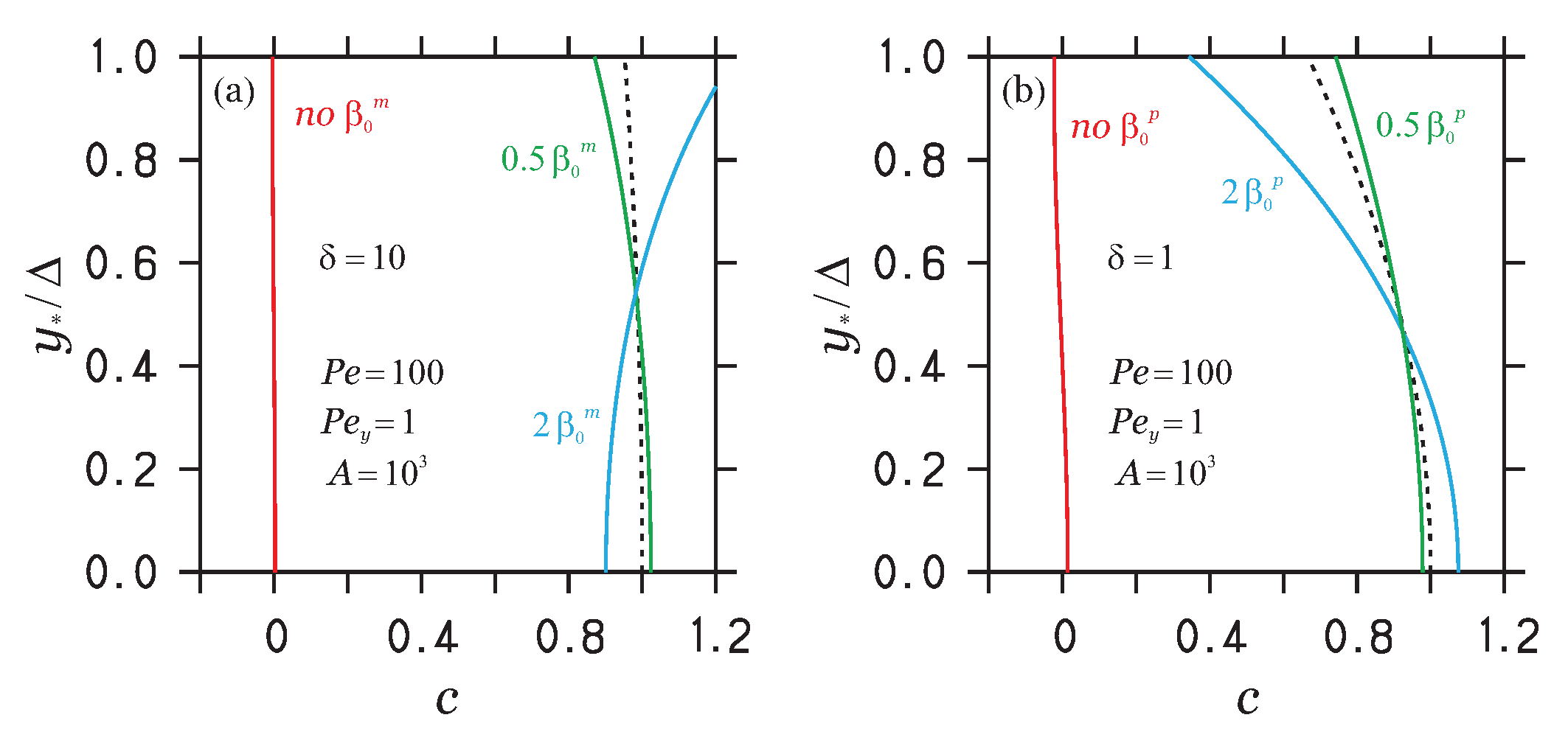
  • Arguably, our most relevant observation is that p = 2 ( 1 P e y / P e c ) / δ , which separates different eigenvalue regimes and also separates different mass transport regimes, in particular diffusion ( p > 0 , y 2 y 1 < L f ) and advection ( p < 0 , y 2 y 1 > L f )-dominated regimes. These regime separation conditions compare geometric conditions (the domain size) with the characteristic length scale L f imposed by the flow. Given a membrane size considered, knowledge of the regime separation conditions is beneficial for the understanding of upscaling requirements, i.e., the use of lab results for pilot- and full-scale applications; with respect to the same flow properties, upscaling can imply transitions from very efficient to very inefficient flow regimes. A very relevant observation is that diffusion-dominated and advection-dominated flow regimes correspond to unblocked (low concentration values) and blocked (high concentration values) flow. Hence, the mathematical characterization of the dominance of one process has relevant physical consequences. Advection-dominated flow implies blocked flow because the dominance of advection inhibits molecular diffusion, i.e., the reduction in concentration gradients.
  • Knowledge of analytical equivalence conditions for A, P e and P e y parameter variations for cases of practical relevance enables the use of various parameter variations to realize desired effects (under conditions where certain parameter variations are inappropriate). The understanding of several ways to accomplish regime changes enables transitions to preferred flow regimes (see the discussion related to Figure 7). The ZOM can provide exact conclusions about equivalent variations of OCs.
  • The FSM, but in particular the ZOM, provide an answer to question Q3 about the understanding of the overall mass transport and characteristic mass distribution features: for both flow regimes, the ZOM explains the difference between (input and output) boundary values implied by OCs and characteristic concentration variations in between these bounds. In particular, the ZOM enables the explicit calculation of global maximum/minimum concentration values c 1 ( 1 P e y / [ P e y + 2 δ ] ) X 0 ( x 2 ) s 0 ( x , y ) c 1 , which is helpful for the understanding of concentration variations.
  • Based on the FSM, the ZOM s 0 ( x , y ) = f ( y ) X 0 ( x ) was presented, which be can be easily applied. The ZOM performance was found to be excellent for all regimes of practical relevance; see above. The significant advantages offered by the ZOM are described above (see second and third points).
  • According to Equation (2), the mass transport is affected by mass transport properties (diffusivity D c ^ ), mass transport initial and BCs, and the structure of the velocity field. The transport properties are known, and there is no problem to exactly satisfy mass transport initial and BCs. Although the velocity field is only approximately represented, the boundedness property of mass transport ensures then proper transitions between the imposed exact BCs, i.e., more complex flow conditions can be covered by the method considered.
Our conclusions support the membrane system design via providing relevant guidelines for applications; see the preceding paragraph, in particular the conclusions regarding questions Q1–Q3. It can be expected that the results obtained provide valuable guidelines for CFD and experimental studies, even under conditions where spacers and other effects are present (see the conclusion to question Q5). Direct applications of our method to membrane system design are not the scope of our paper, the latter requires extensive comparisons with corresponding CFD results for a wide range of parameter variations.
The results presented may be seen as modeling of the solute concentration of oil-in an oil-in-water emulsion (see the reference to a corresponding stochastic particle system in Section 2.1). However, in fact, the same equations can be used to model a variety of other systems, as, for example, saltwater systems for brackish water and seawater reverse osmosis. It is worth noting that the method presented actually represents a design strategy that can be applied to other (radial) geometries; it can be extended to three-dimensional analyses, and it can be applied with other initial and boundary conditions. Results obtained on this basis can be expected to provide valuable additional information and conclusions in support of numerical and experimental studies of membrane systems.

Author Contributions

Conceptualization, S.H.; Methodology, J.A.B.; Software, J.H.; Validation, J.H.; Formal analysis, S.H. and J.H.; Investigation, J.H.; Resources, J.A.B.; Data curation, J.H.; Writing—original draft, S.H.; Writing—review & editing, J.H. and J.A.B.; Visualization, J.H.; Supervision, S.H. and J.A.B.; Project administration, J.A.B.; Funding acquisition, J.A.B. All authors have read and agreed to the published version of the manuscript.

Funding

This research was funded by the United States Department of Energy (DOE) grant number DE-FE0031855.

Institutional Review Board Statement

Not applicable.

Informed Consent Statement

Not applicable.

Data Availability Statement

Not applicable.

Acknowledgments

The authors gratefully acknowledge the financial support for this work that was provided by the United States Department of Energy (DOE) under the following Federal Grant Number: DE-FE0031855.

Conflicts of Interest

The authors declare no conflict of interest.

Nomenclature

Aaspect ratio, x 2 / ( y 2 y 1 )
cdispersed phase concentration
c i n initial value in c ( x , y , 0 ) = c i n
c 1 model parameter, see Equation (A13)
D M molecular diffusion coefficient
D c capillary diffusion coefficient
D c ^ D c / ϵ p
f ( y ) imposed boundary condition
g ( x , y ) imposed initial condition
L f characteristic length, P e c D c ^ / V ^
P e Péclet number, U ^ x 2 / D c ^
P e y Péclet number, V ^ ( y 2 y 1 ) / D c ^
P e c critical Péclet number, 4 / ( 2 + δ )
pparameter, 2 / δ ( 1 + 2 / δ ) P e y / 2
Rparameter, [ 1 + ( 1 + β n 2 ) U 2 / V 2 ] 1 / 2
s , w stationary, transitional solutions
ttime
t non-dim., V ^ 2 t / ( 4 D c ^ )
U n shifted y eigenfunction
U , V velocities in x , y directions
U / V non-dim., P e / ( A P e y )
U ^ , V ^ U / ϵ p , V / ϵ p
X n x eigenfunction
x , y positions in space
x 1 , x 2 x domain bounds
y 1 , y 2 y domain bounds
x , y non-dim., U ^ x / ( 2 D c ^ ) , V ^ y / ( 2 D c ^ )
x 2 non-dim., U ^ x 2 / ( 2 D c ^ ) = P e / 2
y 1 , y 2 non-dim., V ^ y 1 / ( 2 D c ^ ) , V ^ y 2 / ( 2 D c ^ )
β 0 , β 0 m , β 0 p eigenvalues, see Equations (12) and (13)
Δ non-dim., y 2 y 1 = P e y / 2
δ 1 membrane permeability in Equation (4)
ϵ p membrane porosity
ν kinematic viscosity
( ) m i n , m a x minimum, maximum values
( ) 0 zeroth order contributions

Appendix A. Stationary and Transitional Solutions

Appendix A.1. Stationary Solution

The stationary solution satisfies the stationary partial differential equation
2 U 2 V 2 s x + 2 s y = U 2 V 2 2 s x 2 + 2 s y 2 ,
combined with non-homogeneous BCs,
s ( 0 , y ) = f ( y ) , s x ( x 2 , y ) = 0 , s y ( x , y 1 ) = 0 , s ( x , y 2 ) + δ 2 s y ( x , y 2 ) = 0 .
The solution s ( x , y ) of Equation (A1) can be obtained by separation of variables [56]. It reads
s ( x , y ) = n = 0 N s n = e y n = 0 N a n X n ( x ) U n ( y ) ,
where N is supposed. The x eigenfunctions, which read the eigenvalues β n of y eigenfunctions, are given by
X n ( x ) = e ( 1 R ) x 1 + R ( 1 R ) e 2 R ( x 2 x ) 1 + R ( 1 R ) e 2 R x 2 ,
where R = [ 1 + ( 1 + β n 2 ) U 2 / V 2 ] 1 / 2 . Equation (A3) applies the modification Y n ( y ) = e y U n ( y ) of y eigenfunctions, which simplifies the ordinary differential equation (ODE) for y eigenfunctions because of a vanishing first-order derivative. For n = 1 , 2 , , the modified eigenfunctions are found to be given by
U n ( y ) = β n c o s β n ( y y 1 ) s i n β n ( y y 1 ) .
For the case n = 1 , 2 , considered, the y eigenvalues β n satisfy the equation
π 1 β n ( y 2 y 1 ) n = π 1 a r c t a n β n 1 + δ ( 1 + β n 2 ) / 2 .
This equation can be solved iteratively starting with β n = n π / ( y 2 y 1 ) on the right-hand side (RHS). The solution is obtained after fewer than 20 iterations. The converged solution can be written β n = ν π / ( y 2 y 1 ) , where ν refers to the shifted eigenvalue (in contrast to n). Depending on the BCs (the setting of δ ), it turns out that ν is bounded, n ν n + 1 / 2 . Here, the lower and upper limits correspond to δ and δ = 0 , respectively.
However, there are also contributions for n = 0 . In particular, these contributions are determined by the sign of p = 2 / δ ( 1 + 2 / δ ) Δ , where Δ = y 2 y 1 is applied [56]. Here, p arises from the BCs of U [56]. One finds 0 = U ( y 1 ) p 1 U ( y 1 ) and 0 = U ( y 2 ) + p 2 U ( y 2 ) , where p 1 = 1 and p 2 = 1 + 2 / δ . The latter implies p = p 1 + p 2 + p 1 p 2 Δ . Let us consider these two cases in the following two paragraphs (the consideration of p = 0 has little practical value because it implies a specific setting for Δ which can be avoided).
(a) Case p > 0 : In this case, there is one additional positive eigenvalue (denoted by β 0 p , p refers to a positive eigenvalue) below β 1 = π / ( y 2 y 1 ) . The eigenfunction follows Equation (A5),
U 0 p ( y ) = β 0 p c o s β 0 p ( y y 1 ) s i n β 0 p ( y y 1 ) .
The eigenvalue β 0 p is determined by the solution of Equation (A6) with n = 0 ,
β 0 p ( y 2 y 1 ) = a r c t a n β 0 p 1 + δ ( 1 + [ β 0 p ] 2 ) / 2 .
This equation was solved iteratively in the same way as Equation (A6) by applying, however, 1000 iterations starting with β 0 m = 10 8 .
(b) Case p < 0 : In this case, there is one additional negative eigenvalue (denoted by β 0 m , m refers to a negative eigenvalue). The corresponding eigenfunction reads
U 0 m ( y ) = β 0 m c o s h [ β 0 m ( y y 1 ) ] s i n h [ β 0 m ( y y 1 ) ] = = γ 1 2 e β 0 m ( y y 1 ) + γ + 1 2 e β 0 m ( y y 1 ) ,
where β 0 m is given by the solution of
β 0 m ( y 2 y 1 ) = a r c t a n h β 0 m 1 + δ ( 1 [ β 0 m ] 2 ) / 2 .
An alternative formulation of this equation, which is based on the solution of the quadratic equation for β 0 m , reads
β 0 m = 1 δ t a n h ( β 0 m Δ ) + 1 δ 2 t a n h 2 ( β 0 m Δ ) + 1 + 2 δ .
The latter equation was found to deal correctly with the limit β 0 m 1 . It was numerically solved in the same way as Equation (A8) by applying 1000 iterations starting with β 0 m = 10 6 .
The coefficients a n in Equation (A3) are chosen such that the stationary solution s matches an imposed boundary function f ( y ) at x = 0 ; this means s ( 0 , y ) = f ( y ) . The key for deriving the coefficient formula is to make use of the orthogonality of U n ( y ) eigenfunction, y 1 y 2 U n ( y ) U m ( y ) d y = δ n m w n 2 , where the squared norm w n 2 of U n is given in Table A1.
Table A1. Fourier coefficients a n and a 0 m of the stationary solution, where a 0 p = a 0 .
Positive eigenvalues
a n = c 1 s i n ( β n Δ ) w n 2 e y 2 c 1 e y 2 k 1 n c o s ( β n Δ ) + k 2 n s i n ( β n Δ ) 4 β n e y 1 w n 2 Δ ( Δ + δ ) ( 1 + β n 2 ) 2 ,
k 1 n = 2 β n 2 + ( 1 + β n 2 ) Δ , k 2 n = 1 2 β n 2 + 1 + ( 1 + β n 2 ) Δ 2 ,
w n 2 = 1 + β n 2 2 Δ 1 β n 2 4 β n s i n ( 2 β n Δ ) + 1 2 c o s ( 2 β n Δ ) 1 2
Negative eigenvalue
a 0 m = c 1 s i n h ( β 0 m Δ ) w m 2 e y 2 c 1 e y 2 k 1 m c o s h ( β 0 m Δ ) + k 2 m s i n h ( β 0 m Δ ) 4 β 0 m e y 1 w m 2 Δ ( Δ + δ ) ( 1 [ β 0 m ] 2 ) 2 ,
k 1 m = 2 β 0 m 2 + ( 1 [ β 0 m ] 2 ) Δ , k 2 m = 1 + 2 [ β 0 m ] 2 + 1 + ( 1 [ β 0 m ] 2 ) Δ 2 ,
w m 2 = 1 2 1 [ β 0 m ] 2 2 Δ + ( 1 β 0 m ) 2 8 β 0 m e 2 β 0 m Δ ( 1 + β 0 m ) 2 8 β 0 m e 2 β 0 m Δ
By using this property, one obtains
a n = 1 w n 2 y 1 y 2 e y f ( y ) U n ( y ) d y .
The requirement for the imposed function f ( y ) is that it needs to satisfy the BCs. In order to do so, it is assumed that
f ( y ) = c 1 1 ( y y 1 ) 2 Δ ( Δ + δ ) .
The use of this expression in Equation (A12) provides a n as given in Table A1. The abbreviations a 0 p and a 0 m are used to refer to the coefficients related to positive and negative eigenvalues, respectively. It is worth noting that w n 2 and w m 2 refer to the squared norm of U n and U 0 m , respectively. In correspondence to the notation used before, w 0 2 refers to the squared norm of U 0 p . With respect to a 0 m , there arises a question about the limit β 0 m 1 , which is relevant to some parameter regimes. In this limit case, one finds a 0 m to be given by
a 0 m = c 1 s i n h ( β 0 m Δ ) w m 2 e y 2 c 1 1 e 2 Δ ( 1 + 2 Δ + 2 Δ 2 ) 4 w m 2 Δ ( Δ + δ ) e y 1 .
The latter expression was applied for | β 0 m 1 | 10 8 . The model (A3) obtained in this way represents the stationary Fourier series model (FSM).

Appendix A.2. Transitional Solution

The transitional solution satisfies the non-stationary equation,
w t + 2 U 2 V 2 w x + 2 w y = U 2 V 2 2 w x 2 + 2 w y 2 ,
combined with homogeneous BCs,
w ( 0 , y , t ) = w x ( x 2 , y , t ) = w y ( x , y 1 , t ) = 0 , w ( x , y 2 , t ) + δ 2 w y ( x , y 2 , t ) = 0 ,
and the initial condition w ( x , y ) = g ( x , y ) . The solution w ( x , y , t ) of Equation (A15) can be found via separation of variables. It is given by
w ( x , y , t ) = c i n w 1 ( x , t ) w 2 ( y , t ) ,
where (by supposing N and M )
w 1 ( x , t ) = m = 1 M c m s i n α m x e x p x ( 1 + α m 2 ) [ U / V ] 2 t ,
w 2 ( y , t ) = = n = 0 N b n β n c o s β n ( y y 1 ) s i n β n ( y y 1 ) e x p y ( 1 + β n 2 ) t .
With respect to w 2 ( y , t ) , the terms of zeroth order are provided in dependence on p as described above regarding the stationary solution; see cases (a) and (b). This means, for p > 0 Equation (A19) is applied, whereas s i n [ ] and c o s [ ] are replaced by the corresponding s i n h [ ] and c o s h [ ] functions for p < 0 .
In consistency with Table A1, the y Fourier coefficients (which were determined by the condition to integrate to one, meaning no initial y variation was considered) are given in Table A2.
Table A2. y Fourier coefficients b n and b 0 m of the transitional solution ( b 0 p = b 0 ).
Positive eigenvalues
b n = s i n ( β n Δ ) w n 2 e y 2 , w n 2 = 1 + β n 2 2 Δ 1 β n 2 4 β n s i n ( 2 β n Δ ) + 1 2 c o s ( 2 β n Δ ) 1 2
Negative eigenvalue
b 0 m = s i n h ( β 0 m Δ ) w m 2 e y 2 , w m 2 = 1 [ β 0 m ] 2 2 Δ + 1 + [ β 0 m ] 2 4 β 0 m s i n h ( 2 β 0 m Δ ) 1 2 c o s h ( 2 β 0 m Δ ) + 1 2
The corresponding x Fourier coefficients can be calculated on the basis of the orthogonality property of x eigenfunctions, 0 x 2 s i n α n x s i n α m x d x = δ n m w x 2 , where the squared norm of x eigenfunctions is given by
w x 2 = x 2 2 s i n ( 2 α m x 2 ) 4 α m .
The x eigenvalues α m in Equation (A18) satisfy the equation
π 1 α m x 2 n = π 1 a r c t a n ( α m ) .
Here, n = 1 , 2 , refers to non-disturbed eigenvalue numbers. The technique to solve this equation for n = 1 , 2 , is equivalent to the solution of Equation (A6) related to the stationary solution, where 20 iterations were applied. There is one positive eigenvalue below α 1 = π / x 2 which is included in the solution of Equation (A22) for n = 1 , 2 , .
With respect to the x Fourier coefficients, the condition reads
c m = 1 w x 2 0 x 2 e x g ( x ) s i n ( α m x ) d x ,
where g ( x ) is an imposed x profile. Regarding the latter,
g ( x ) = c i n e x x 2 1 + ( x 2 x ) ( 1 + 1 / x 2 ) x / x 2
is applied. This function follows the e x variation of w 1 ( x , t ) ; the factor e x 2 is included for normalization. The function g ( x ) is positive, bounded, and correctly satisfies the x BCs; this means g ( 0 ) = 0 and g ( x 2 ) = 0 . By using Equation (A22), the x Fourier coefficients obtained read
c m = 2 ( 1 + 1 / x 2 ) e x 2 x 2 w x 2 α m 3 1 c o s ( α m x 2 ) .
The model Equation (A17) obtained represents the transitional Fourier series model (FSM).

References

  1. Gruber, M.F.; Johnson, C.J.; Tang, C.Y.; Jensen, M.H.; Yde, L.; Hélix-Nielsen, C. Computational fluid dynamics simulations of flow and concentration polarization in forward osmosis membrane systems. J. Membr. Sci. 2011, 379, 488–495. [Google Scholar] [CrossRef]
  2. Gruber, M.F.; Johnson, C.J.; Tang, C.Y.; Jensen, M.H.; Yde, L.; Hélix-Nielsen, C. Validation and analysis of forward osmosis CFD model in complex 3D geometries. Membranes 2012, 2, 764–782. [Google Scholar] [CrossRef] [PubMed] [Green Version]
  3. Gruber, M.F.; Aslak, U.; Hélix-Nielsen, C. Open-source CFD model for optimization of forward osmosis and reverse osmosis membrane modules. Sep. Purif. Technol. 2016, 158, 183–192. [Google Scholar] [CrossRef] [Green Version]
  4. Rahimi, M.; Madaeni, S.S.; Abolhasani, M.; Alsairafi, A.A. CFD and experimental studies of fouling of a microfiltration membrane. Chem. Eng. Process. Process Intensif. 2009, 48, 1405–1413. [Google Scholar] [CrossRef]
  5. Zare, M.; Ashtiani, F.Z.; Fouladitajar, A. CFD modeling and simulation of concentration polarization in microfiltration of oil–water emulsions; Application of an Eulerian multiphase model. Desalination 2013, 324, 37–47. [Google Scholar] [CrossRef]
  6. Lotfiyan, H.; Ashtiani, F.Z.; Fouladitajar, A.; Armand, S.B. Computational fluid dynamics modeling and experimental studies of oil-in-water emulsion microfiltration in a flat sheet membrane using Eulerian approach. J. Membr. Sci. 2014, 472, 1–9. [Google Scholar] [CrossRef]
  7. Tashvigh, A.A.; Fouladitajar, A.; Ashtiani, F.Z. Modeling concentration polarization in crossflow microfiltration of oil-in-water emulsion using shear-induced diffusion; CFD and experimental studies. Desalination 2015, 357, 225–232. [Google Scholar] [CrossRef]
  8. Zoubeik, M.; Salama, A.; Henni, A. A novel antifouling technique for the crossflow filtration using porous membranes: Experimental and CFD investigations of the periodic feed pressure technique. Water Res. 2018, 146, 159–176. [Google Scholar] [CrossRef]
  9. Behroozi, A.H.; Kasiri, N.; Mohammadi, T. Multi-phenomenal macroscopic investigation of cross-flow membrane flux in microfiltration of oil-in-water emulsion, experimental & computational. J. Water Process. Eng. 2019, 32, 100962. [Google Scholar]
  10. Behroozi, A.H. A modified resistance model for simulating baffle arrangement impacts on cross–flow microfiltration performance for oily wastewater. Chem. Eng. Process. Process Intensif. 2020, 153, 107962. [Google Scholar] [CrossRef]
  11. Alshwairekh, A.M.; Alghafis, A.A.; Alwatban, A.M.; Alqsair, U.F.; Oztekin, A. The effects of membrane and channel corrugations in forward osmosis membrane modules–Numerical analyses. Desalination 2019, 460, 41–55. [Google Scholar] [CrossRef]
  12. Schwinge, J.; Wiley, D.E.; Fletcher, D.F. Simulation of the flow around spacer filaments between narrow channel walls. 1. Hydrodynamics. Ind. Eng. Chem. Res. 2002, 41, 2977–2987. [Google Scholar] [CrossRef]
  13. Schwinge, J.; Wiley, D.E.; Fletcher, D.F. Simulation of the flow around spacer filaments between channel walls. 2. Mass-transfer enhancement. Ind. Eng. Chem. Res. 2002, 41, 4879–4888. [Google Scholar] [CrossRef]
  14. Schwinge, J.; Neal, P.R.; Wiley, D.E.; Fletcher, D.F.; Fane, A.G. Spiral wound modules and spacers: Review and analysis. J. Membr. Sci. 2004, 242, 129–153. [Google Scholar] [CrossRef]
  15. Song, L.; Ma, S. Numerical studies of the impact of spacer geometry on concentration polarization in spiral wound membrane modules. Ind. Eng. Chem. Res. 2005, 44, 7638–7645. [Google Scholar] [CrossRef]
  16. Siddiqui, A.; Lehmann, S.; Haaksman, V.; Ogier, J.; Schellenberg, C.; Van Loosdrecht, M.C.M.; Kruithof, J.C.; Vrouwenvelder, J.S. Porosity of spacer-filled channels in spiral-wound membrane systems: Quantification methods and impact on hydraulic characterization. Water Res. 2017, 119, 304–311. [Google Scholar] [CrossRef] [Green Version]
  17. Mojab, S.M.; Pollard, A.; Pharoah, J.G.; Beale, S.B.; Hanff, E.S. Unsteady laminar to turbulent flow in a spacer-filled channel. Flow Turbul. Combust. 2014, 92, 563–577. [Google Scholar] [CrossRef]
  18. Ranade, V.V.; Kumar, A. Fluid dynamics of spacer filled rectangular and curvilinear channels. J. Membr. Sci. 2006, 271, 1–15. [Google Scholar] [CrossRef] [Green Version]
  19. Ranade, V.V.; Kumar, A. Comparison of flow structures in spacer-filled flat and annular channels. Desalination 2006, 191, 236–244. [Google Scholar] [CrossRef]
  20. Keir, G.; Jegatheesan, V. A review of computational fluid dynamics applications in pressure-driven membrane filtration. Rev. Environ. Sci. Bio Technol. 2014, 13, 183–201. [Google Scholar] [CrossRef]
  21. Fimbres-Weihs, G.A.; Wiley, D.E. Review of 3D CFD modeling of flow and mass transfer in narrow spacer-filled channels in membrane modules. Chem. Eng. Process. Process Intensif. 2010, 49, 759–781. [Google Scholar] [CrossRef]
  22. Lau, K.K.; Abu Bakar, M.Z.; Ahmad, A.L.; Murugesan, T. Effect of feed spacer mesh length ratio on unsteady hydrodynamics in 2d spiral wound membrane (swm) channel. Ind. Eng. Chem. Res. 2010, 49, 5834–5845. [Google Scholar] [CrossRef]
  23. Kostoglou, M.; Karabelas, A.J. On the fluid mechanics of spiral-wound membrane modules. Ind. Eng. Chem. Res. 2009, 48, 10025–10036. [Google Scholar] [CrossRef]
  24. Koutsou, C.P.; Karabelas, A.J.; Kostoglou, M. Fluid dynamics and mass transfer in spacer-filled membrane channels: Effect of uniform channel-gap reduction due to fouling. Fluids 2018, 3, 12. [Google Scholar] [CrossRef] [Green Version]
  25. Kavianipour, O.; Ingram, G.D.; Vuthaluru, H.B. Investigation into the effectiveness of feed spacer configurations for reverse osmosis membrane modules using Computational Fluid Dynamics. J. Membr. Sci. 2017, 526, 156–171. [Google Scholar] [CrossRef] [Green Version]
  26. Kavianipour, O.; Ingram, G.D.; Vuthaluru, H.B. Studies into the mass transfer and energy consumption of commercial feed spacers for RO membrane modules using CFD: Effectiveness of performance measures. Chem. Eng. Res. Des. 2019, 141, 328–338. [Google Scholar] [CrossRef]
  27. Horstmeyer, N.; Lippert, T.; Schön, D.; Schlederer, F.; Picioreanu, C.; Achterhold, K.; Pfeiffer, F.; Drewes, J. CT scanning of membrane feed spacers–Impact of spacer model accuracy on hydrodynamic and solute transport modeling in membrane feed channels. J. Membr. Sci. 2018, 564, 133–145. [Google Scholar] [CrossRef]
  28. Liang, Y.Y.; Toh, K.Y.; Fimbres-Weihs, G.A. 3D CFD study of the effect of multi-layer spacers on membrane performance under steady flow. J. Membr. Sci. 2019, 580, 256–267. [Google Scholar] [CrossRef]
  29. Liang, Y.Y.; Fimbres Weihs, G.A.; Wiley, D.E. Comparison of oscillating flow and slip velocity mass transfer enhancement in spacer-filled membrane channels: CFD analysis and validation. J. Membr. Sci. 2020, 593, 117433. [Google Scholar] [CrossRef]
  30. Foo, K.; Liang, Y.Y.; Tan, C.K.; Fimbres Weihs, G.A. Coupled effects of circular and elliptical feed spacers under forced-slip on viscous dissipation and mass transfer enhancement based on CFD. J. Membr. Sci. 2021, 637, 119599. [Google Scholar] [CrossRef]
  31. Appadu, A.R. Numerical solution of the 1D advection-diffusion equation using standard and nonstandard finite difference schemes. J. Appl. Math. 2013, 2013. [Google Scholar] [CrossRef]
  32. Smith, R. Optimal and near–optimal advection–diffusion finite–difference schemes I. Constant coefficient in one dimension. Proc. R. Soc. Lond. Ser. A 1999, 455, 2371–2387. [Google Scholar] [CrossRef]
  33. Smith, R. Optimal and near-optimal advection–diffusion finite-difference schemes. II. Unsteadiness and non-uniform grid. Proc. R. Soc. Lond. Ser. A 2000, 456, 489–502. [Google Scholar] [CrossRef]
  34. Smith, R. Optimal and near-optimal advection—diffusion finite-difference schemes III. Black—Scholes equation. Proc. R. Soc. Lond. Ser. A 2000, 456, 1019–1028. [Google Scholar] [CrossRef]
  35. Smith, R. Optimal and near-optimal advection-diffusion finite-difference schemes. IV. Spatial non–uniformity. Proc. R. Soc. Lond. Ser. A 2001, 457, 45–65. [Google Scholar] [CrossRef]
  36. Smith, R.; Tang, Y. Optimal and near–optimal advection–diffusion finite–difference schemes. V. Error propagation. Proc. R. Soc. Lond. Ser. A 2001, 457, 803–816. [Google Scholar] [CrossRef]
  37. Smith, R.; Tang, Y. Optimal and near–optimal advection–diffusion finite–difference schemes. VI Two–dimensional alternating directions. Proc. R. Soc. Lond. Ser. A 2001, 457, 2379–2396. [Google Scholar] [CrossRef]
  38. Smith, R. Optimal and near–optimal advection—diffusion finite–difference schemes. VII Radionuclide chain transport. Proc. R. Soc. Lond. Ser. A 2001, 457, 2719–2740. [Google Scholar] [CrossRef]
  39. Flotron, S.; Rappaz, J. Conservation schemes for convection-diffusion equations with Robin boundary conditions. ESAIM. Math. Model. Numer. Anal. 2013, 47, 1765–1781. [Google Scholar] [CrossRef]
  40. Singh, K.M.; Tanaka, M. Dual reciprocity boundary element analysis of transient advection-diffusion. Int. J. Numer. Methods Heat Fluid Flow 2003, 13, 633–646. [Google Scholar] [CrossRef]
  41. Mokhtarpoor, R.; Heinz, S.; Stoellinger, M. Dynamic unified RANS-LES simulations of high Reynolds number separated flows. Phys. Fluids 2016, 28, 095101/1–095101/36. [Google Scholar] [CrossRef]
  42. Mokhtarpoor, R.; Heinz, S. Dynamic large eddy simulation: Stability via realizability. Phys. Fluids 2017, 29, 105104/1–105104/22. [Google Scholar] [CrossRef] [Green Version]
  43. Heinz, S. The large eddy simulation capability of Reynolds-averaged Navier-Stokes equations: Analytical results. Phys. Fluids 2019, 31, 021702/1–021702/6. [Google Scholar] [CrossRef]
  44. Heinz, S.; Mokhtarpoor, R.; Stoellinger, M. Theory-Based Reynolds-Averaged Navier-Stokes Equations with Large Eddy Simulation Capability for Separated Turbulent Flow Simulations. Phys. Fluids 2020, 32, 065102/1–065102/20. [Google Scholar] [CrossRef]
  45. Heinz, S. A review of hybrid RANS-LES methods for turbulent flows: Concepts and applications. Prog. Aerosp. Sci. 2020, 114, 100597/1–100597/25. [Google Scholar] [CrossRef]
  46. Heinz, S. The Continuous Eddy Simulation Capability of Velocity and Scalar Probability Density Function Equations for Turbulent Flows. Phys. Fluids 2021, 33, 025107/1–025107/13. [Google Scholar] [CrossRef]
  47. Heinz, S.; Peinke, J.; Stoevesandt, B. Cutting-Edge Turbulence Simulation Methods for Wind Energy and Aerospace Problems. Fluids 2021, 6, 288. [Google Scholar] [CrossRef]
  48. Heinz, S. Minimal error partially resolving simulation methods for turbulent flows: A dynamic machine learning approach. Phys. Fluids 2022, 34, 051705/1–051705/7. [Google Scholar] [CrossRef]
  49. Verrall, D.P.; Read, W.W. A quasi-analytical approach to the advection–diffusion–reaction problem, using operator splitting. Appl. Math. Model. 2016, 40, 1588–1598. [Google Scholar] [CrossRef]
  50. Huysmans, M.; Dassargues, A. Review of the use of Péclet numbers to determine the relative importance of advection and diffusion in low permeability environments. Hydrogeol. J. 2005, 13, 895–904. [Google Scholar] [CrossRef] [Green Version]
  51. Phattaranawik, J.; Jiraratananon, R.; Fane, A.G.; Halim, C. Mass flux enhancement using spacer filled channels in direct contact membrane distillation. J. Membr. Sci. 2001, 187, 193–201. [Google Scholar] [CrossRef]
  52. Yun, Y.; Wang, J.; Ma, R.; Fane, A.G. Effects of channel spacers on direct contact membrane distillation. Desalin. Water Treat. 2011, 34, 63–69. [Google Scholar] [CrossRef]
  53. Tirabassi, T.; Buske, D.; Moreira, D.M.; Vilhena, M.T. A two-dimensional solution of the advection–diffusion equation with dry deposition to the ground. J. Appl. Meteorol. Climatol. 2008, 47, 2096–2104. [Google Scholar] [CrossRef]
  54. McKee, S.; Dougall, E.A.; Mottram, N.J. Analytic solutions of a simple advection-diffusion model of an oxygen transfer device. J. Math. Ind. 2016, 6, 1–22. [Google Scholar] [CrossRef]
  55. Bird, R.B.; Stewart, W.E.; Lightfoot, E.N. Transport Phenomena, 2nd ed.; John Wiley & Sons: New York, NY, USA, 2006. [Google Scholar]
  56. Strauss, W.A. Partial Differential Equations: An Introduction; John Wiley & Sons: New York, NY, USA, 1992. [Google Scholar]
  57. Heinz, S. Mathematical Modeling; Springer: Heidelberg, Gemany, 2011. [Google Scholar]
  58. WolframAlpha. Available online: https://www.wolframalpha.com/input (accessed on 3 October 2022).
Figure 1. Membrane system illustration.
Fluids 07 00369 g001
Figure 4. Parameter regimes: the black curve shows P e y values for which p = 2 / δ ( 1 + 2 / δ ) P e y / 2 = 0 .
Fluids 07 00369 g004
Figure 8. Eigenvalues β 0 m and β 0 p as function of (a) P e y (depending on δ ) and (b) δ (depending on P e y ). The vertical lines separate β 0 m from β 0 p .
Fluids 07 00369 g008
Publisher’s Note: MDPI stays neutral with regard to jurisdictional claims in published maps and institutional affiliations.

