Article

Deep Learning Forecasts a Strained Turbulent Flow Velocity Field in Temporal Lagrangian Framework: Comparison of LSTM and GRU

by
Reza Hassanian
1,2,*,
Ásdís Helgadóttir
1,2 and
Morris Riedel
1,3
1
The Faculty of Industrial Engineering, Mechanical Engineering and Computer Science, University of Iceland, 102 Reykjavík, Iceland
2
Computational Fluid Dynamics, Simulation and Data Lab, National Competence Centre of Iceland, University of Iceland, 102 Reykjavík, Iceland
3
Juelich Supercomputing Centre, 52428 Jülich, Germany
*
Author to whom correspondence should be addressed.
Fluids 2022, 7(11), 344; https://doi.org/10.3390/fluids7110344
Submission received: 15 September 2022 / Revised: 27 October 2022 / Accepted: 1 November 2022 / Published: 3 November 2022
(This article belongs to the Special Issue Machine Learning in Fluid Flow and Heat Transfer)

Abstract

:
The subject of this study presents an employed method in deep learning to create a model and predict the following period of turbulent flow velocity. The applied data in this study are extracted datasets from simulated turbulent flow in the laboratory with the Taylor microscale Reynolds numbers in the range of 90 < R λ < 110. The flow has been seeded with tracer particles. The turbulent intensity of the flow is created and controlled by eight impellers placed in a turbulence facility. The flow deformation has been conducted via two circular flat plates moving toward each other in the center of the tank. The Lagrangian particle-tracking method has been applied to measure the flow features. The data have been processed to extract the flow properties. Since the dataset is sequential, it is used to train long short-term memory and gated recurrent unit model. The parallel computing machine DEEP-DAM module from Juelich supercomputer center has been applied to accelerate the model. The predicted output was assessed and validated by the rest of the data from the experiment for the following period. The results from this approach display accurate prediction outcomes that could be developed further for more extensive data documentation and used to assist in similar applications. The mean average error and R2 score range from 0.001–0.002 and 0.9839–0.9873, respectively, for both models with two distinct training data ratios. Using GPUs increases the LSTM performance speed more than applications with no GPUs.

1. Introduction

Turbulent flow is a nonlinear and random phenomenon [1,2,3]. Water flow in a river, waterfall, airflow passing a wind turbine blade, flow in an engine mixing chamber, smoke from a chimney, and two working flows inside the heat exchanger are examples of turbulent flow in natural events and artificial applications [1,2,3,4,5]. The complexity and multiscale features of turbulent flows make the forecasting of the fluid flow a considerable problem. There are many previous works using experiments and/or numerical methods of turbulent flow to investigate and make efforts to forecast flow periods with specified conditions. However, experiments are costly and, for many applications, could not be performed in a laboratory environment. Computational methods based on partial differential equations, i.e., applying a full-order model, are capable of predicting fluid flow accurately but are computationally costly. High-performance computing is, therefore, essential in those computational methods, yet we are still far from having computing capability to solve even moderately sized problems. Thus, there are limitations in computing costs [6].
These restrictions determine a reliable tool is required to overcome the above-mentioned obstacles. Machine learning based on artificial intelligence has become a pivotal approach to encountering nonlinear events. Deep learning networks (DL) applications have recently been represented as having strong capability to model and forecast phenomena with unknown patterns. DL is able to extract hidden features from complex and nonlinear dynamic systems [7,8]. Recurrent neural networks (RNNs) are neural networks appropriate for sequential datasets, such as time series [7]. An RNN is composed of an individual hidden layer with a feedback loop in which the hidden layer output with the current input is returned to the hidden layer [7]. RNNs define the temporal relationship because of sequential input data and three weight matrices and two biases characterize it. RNNs can almost not train the sequential data with long-range temporal dependencies because a vanishing gradients problem exists [7]. Long short-term memory (LSTM) networks were developed and suggested in 1995 [9], which apply a gating structure to control the recurrent connectors’ transients and deal with a vanishing gradient issue. Moreover, it is able to model longer temporal dependencies than standard RNNs [7].
A gated recurrent unit (GRU) is a variant of LSTM, which has fewer parameters than LSTM, and its training rate is faster [10,11]. In GRU, the forget gate and input gate in LSTM are replaced with only one update gate [11]. GRU requires fewer data to train the model, therefore, gaining a similar performance in multiple tasks with less computation [11]. Recently, LSTM has been employed in many studies to model time series prediction. Interest in this method has also increased in the fluid dynamics area. Vinuesa et al. [7] have used LSTM to predict a shear turbulence flow. Veisi et al. [8] used LSTM hybrid model prediction for unsteady flows. LSTM potential has led to hybrid models, such as convolutional neural networks (CNNs)-LSTM, Autoencoders-LSTM, and LSTM/RNN [11]. Bukka et al. [6] applied a hybrid deep learning prediction model based on a reduced-order model for unsteady flow. Duru et al. [12] used CNN to predict transonic flow around the airfoils. GRU has been employed to forecast wind speed and anticipate electricity demands [10,11].
Most fluid flow studies that applied ML/DL are composed of data extracted from CFD studies’ known equations. On the other hand, many works include preliminary steps to autoencoders to extract the main features, such as proper orthogonal decomposition, dynamic mode decomposition, and well-known reduced-order methods [8,13,14,15].
The subject of the current study is a novel approach to present a capability in the DL context to make a training method with raw measured data from the Lagrangian framework velocity field with non-specified pattern and to predict followed fluid flow period. In many applications of industry and experiments, it is possible to measure the velocity fields directly or indirectly via devices, such as a constant temperature anemometer, flowmeter (and obtain the velocity), pitot tube, laser doppler anemometry, and light detection and ranging. This study will introduce an application of an empirical dataset from a laboratory with unknown patterns composed of 2D velocity components and time. LSTM and GRU have been used to create a prediction model for a strained turbulent flow. In order to accelerate the deep models’ execution, they were implemented in the DEEP-DAM module from a parallel computing machine at the Juelich supercomputing center. Hence, this paper is organized as follows. The applied theory is introduced in Section 2. In Section 3, the data set from the experiment is explained. Section 4 determines the models used. The results and discussion are provided in Section 5, and the conclusion is presented in Section 6.

2. Theory

2.1. Fluid Flow in Lagrangian Framework

In turbulent flow, it is well-known what statistical aspects of the flow features are applicable [1,2,3]. A Lagrangian framework is an exploration of fluid motion that keeps track of the velocity vector and displacement vector of each flow point, called a fluid particle [1,16]. A fluid particle is a point that moves with the local fluid velocity, and, therefore, it identifies the position at the time t of a fluid particle [16]. The definition of a fluid particle arithmetically is [1]:
x i = x i ( t , x i , 0 ) ,   i = 1 , 2 , 3
U i = U i ( t , x 1 ( t , x 1 , 0 ) , x 2 ( t , x 2 , 0 ) , x 3 ( t , x 3 , 0 ) )
where the fluid particle position and velocity in 3D coordinates is determined by (1) and (2), respectively, x is the position, U is the velocity, t is the time, and i specifies the vector component.
Based on the Lagrangian definition, there is time series data for fluid particles that determine a position and velocity at a specific time. In particular, in turbulent flow, which has no known equation and is investigated using statistics, a sequential dataset could be used from the Lagrangian view for the forecasting model. It is a crucial challenge to be able to have accurate prediction for turbulent flow velocity via an approach that does not need preprocessing to extract hidden features or reduced order methods [6,7,8,17,18,19]. Some numerical methods due have drawbacks, such as missing features because of dimension reduction [6,7,8,17,18,19]. Based on the above description for the velocity in the Lagrangian framework, in this study we will apply velocity denotation (2) to train LSTM or GRU model via velocity component as an input. Then, the model will predict the velocity component for next period as an output.
This study used the dataset for a strained turbulent flow that has been generated in a laboratory. Turbulence intensity has been created with the action of impeller rotors in the corners of a box turbulence facility. The turbulent flow has been strained in the vertical direction (see Figure 1) by the motion of flat circular plates, as shown in the sketch. Equation (3) defines the mean velocity field of the flow:
U = ( Sx , 2 Sy , Sz )
where 2S is the primary strain rate in the Y-dir, S is the mean strain rate for the other two directions, and x, y and z are the particle location. In this work, the flow was considered in 2D, therefore, Z-dir is not addressed.
The straining flow case has been created in the experiment with mean strain rate, 2S = 8 s−1. Equation (3) is based on laminar flow; however, we know that velocity fluctuates in turbulent flow. Further details on the experimental setup are described in Section 3.
The Stokes number for a seeded particle is calculated to ensure a tracer particle meets the requirements and specifies whether a particle introduced to the flow will follow the flow streamline or not. This identification is defined by Equation (4):
St = τ p τ η
where τ p is Stokes’ relaxation time. Kolmogorov scale ( τ η , defined in Equation (6)) is based on the flow quantities before applying the strain. Stokes’ relaxation time τ p is, in turn, calculated by Equation (5):
τ p = ρ p d p 2 18 μ
where ρ p is particle density, d p is a spherical particle diameter, and μ is the dynamic fluid viscosity that, in the conducted experiment, was water.
The Stokes number significantly greater than 1 (St ≫ 1) describes particles that are unaffected by a fluid velocity change and continue their original trajectory; if St ≪ 1, the particle will follow the fluid’s local velocity. To extract the flow properties, particle image velocimetry method has been employed and once dissipation rate specified via second-order longitudinal velocity structure function, Kolmogorov scales were calculated by:
τ η = ( ν ε ) 1 2
where ν is kinematic viscosity of the fluid, τ η is the Kolmogorov’s time scale, and ε is dissipation rate evaluated via second-order longitudinal velocity structure function.
The Stokes number for the tracer particles used in the performed experiment are in the range of 0.0063–0.0094.

2.2. LSTM and GRU Architecture

The subject of this study is using the velocity components U x and U y , according to definition (2) as sequential input training data for LSTM or GRU model. The model for each component is separated. Even though the velocity is a profound feature in the flow field description and is based on the Lagrangian perspective, it is spatiotemporal; therefore, it carries many flow effects, such as fluctuation, strain, turbulence intensity, and geometry boundary [1,2,3,4,5]. This is the capital concept of this novel proposed approach.
Since the flow velocity is spatial-temporal and is affected via the above-nominated effects, the LSTM or GRU model is trained and learns how to forecast the next period according to received effects. The predicted flow velocity via LSTM or GRU model is validated by test data in the x and y components separately.
Recurrent neural networks are deep network models that can extract sequential data dynamics through recurrent connections. They can be considered as cycles in the network of nodes. Although gradient contraction in recurrent neural networks seems to help exploding gradients, handling vanishing gradients requires a more precise solution [20,21,22]. One of the first and most successful techniques to solve the vanishing problems was presented in the long short-term memory model [9].
In simple recurrent neural networks, long-term memory is in the form of weights, and the weights change gradually during the training and encode general knowledge about the data. Additionally, these networks have short-term memory, which is in the form of fast transient activations and is continuously transferred from one node to another. In the LSTM model, an intermediate storage type is defined through a memory cell (see Figure 2). A memory cell is a composite unit that consists of simpler nodes and acts through a specific connectivity pattern by imbedding new multiplicative nodes.
Each memory cell is composed of an internal state and several multiplicative gates, which control the data as follows: (i) a given input should affect the internal state (the input gate) or not, (ii) the internal state should drive to 0 (the forget gate), (iii) a given neuron’s internal state should be able to impact the cell output (the output gate).
A significant distinction between standard RNNs and LSTM is a hidden state gate determined in LSTM. This state provides an appropriate mechanism for when a hidden state should be updated and when it should be reset. These mechanisms are learned, and they resolve the known concerns from standard RNNs. For example, if the first token has a major significance, it will learn not to update the hidden state after the first perception. In addition, it will learn to omit incoherent temporary perceptions. Eventually, it will learn to reset the hidden state whenever it is essential.
GRU is a next-generation determination from LSTM with a bit distinction in the model architecture [23]. Literature reports that GRU is comparable in performance is considerably faster to compute than LSTM and has a streamlined model [17,19,24]. The GRU cell that is displayed in Figure 3 is composed of a hidden state, reset gate, and update gate. We can control how much of the previously hidden state might be remembered from the reset gate.
On the other hand, via the update gate, we can understand how much of the new hidden state is just a copy of the old hidden state. This architecture in the GRU establishes two significant features: the reset gate captures short-term dependencies in sequences and the update gate receives long-term dependencies in sequences [23].

3. Experiment and Dataset

3.1. Apparatus and Experiment Setup

The experiment has been performed at the Laboratory of Fundamental Turbulence Research (LFTR) at Reykjavik University and the applied facility is shown in Figure 4. The water tank (60 cm × 60 cm × 60 cm) has 20 mm thick acrylic walls (transparent Plexiglas XT) that enables optical access to the data. The eight corners of the box have a triangular shape, while the top and the bottom are nearly circular. An aluminum frame holds the components of the turbulence box together. The turbulence has been generated by eight impellers driven by independently controlled servo motors (Lenz-model: MCS), which were mounted at the eight corners of the cube and point to the center of the tank. The rotation rate of each servo motor is adjustable over a range of 100–4500 rpm at a gearing rate of 0.075. For the used dataset in this study the speed is 1000 rpm. The motion-view filtering software that came with these motors was used to monitor and set up the suited speed of each impeller. The degassing system was used to remove bubbles and solid dust from the water before starting the experiment. The tank has been specifically designed for studying turbulence (Lagrangian and Eulerian motion at moderate Reynolds numbers). The flow facility produces a nearly stationary homogeneous isotropic turbulence near the center of the tank, where measurements have been performed.
Circular plates, shown at the top and bottom (see Figure 1), generate the strain motions; a linear actuator drove each plate with a piston rod (Parker, model: ETV32M10PA47JMA400A). When they are moved towards the center with a pre-described rate, a nearly constant strain rate is ensured in the fluid. Spherical and hollow glass beads with a median diameter of 8–10 μm and a specific gravity of 1.1 g/cm3 seed the flow. The recording area is located in the center of the tank with a size of 24.5 × 24.5 mm2 (see Figure 1). The particle image velocimetry technique is applied and extracts the flow properties before strain deformation. Thus, via a second-order longitudinal velocity structure function, the turbulent flow dissipation rate is obtained; therefore, the Kolmogorov time scale is calculated based on Equation (6) and a Stokes number is obtained from Equation (4). The Taylor microscale Reynolds number is achieved in the range of 90 < R λ < 110 in the performed experiment. For the dataset used, the strain rate produced by the two above-described circular plates is 8 s−1, and the Lagrangian particle-tracking techniques are applied to inscribe the data. A high-speed camera used as a detection system was set at 10 kHz (10,000 fps) for well-resolved particle velocity statistics. This very high temporal resolution (0.1–0.2 ms) is considerably smaller than the Kolmogorov time τ η (35–99 ms) of the smallest eddies present in the flow; therefore, the properties of the dissipation range in the flow are resolved. However, in contrast to the previous numerical works, this empirical study considers the velocity field explored by tracer particles in the presence of gravity. Each video has 2000 frames, and to collect sufficient statistical data, the strain motion was repeated 20 times to record 20 videos. All videos together have created 40,000 frames. Each of the videos was statistically independent, as the flow is given a generous time to recover to near isotropy between different strokes.

3.2. Sequential Velocity Dataset

The recorded videos from the experiment are processed via programming based on Lagrangian particle-tracking method and are not subject of this study, and the detail can be seen in [25,26]. Each particle has vector of velocity and displacement during the strain motion. According to denotation (1) and (2) in the Lagrangian view, these statistics could be used to investigate the turbulent flow. As one of the reviewers mentioned, some statistical features can be calculated from extracted data from the experiment [27]. In this study, however, our focus is on velocity because it is a feature that can be measured in many applications, and its prediction model can be helpful. For example, wind speed is a crucial issue in wind energy production; it is, therefore, essential to have a prediction model for speed itself so producers can forecast the power production in the following period, long or short term.
The dataset of this study composed of 2,862,119 tracking points for every vector is as follows:
-
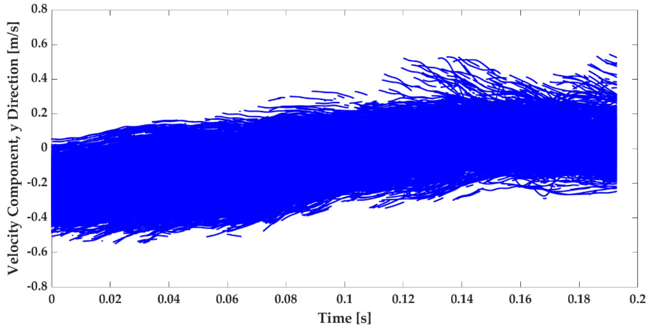
Velocity component in y direction;
-
Velocity component in x direction;
-
Time vector specifies the time t for every tracking point.
These tracking points consist of all particles’ velocity vectors achieved via 20 recordings, and every video recording includes several particles. Moreover, it is expected to observe several tracking lines, as it is presented for the velocity in the results in Section 5; every tracking line specifies a particle.
Although the dataset is sequential, we split it into training data and test data for the first model, 80% and 20%, respectively, and for the second model, 60% and 40%, proportionally. Therefore, we assessed and validated the velocity prediction of the following period with the test data for LSTM and GRU models.

4. LSTM and GRU Model Set Up

We coded the models in Python and used the TensorFlow platform [28,29]. The LSTM model is set up with 100 layers and one dense layer, and Adam is specified as an optimizer. The GRU model has also been set up with the same layers and optimizer. The dataset was normalized by MinMaxScaler transformation [30]. The MinMaxScaler is a type of scaler that scales the minimum and maximum values to be 0 and 1, respectively [30]. Since the modeling was implemented on the DEEP-DAM module [31] parallel computing machine, we have applied a distributed strategy application programming interface from the TensorFlow platform abstraction to distribute the training across multiple custom training loops [32]. The strategy has been set up with one to four GPUs on one node. The result of the computing and the models’ performance distinction are reported in Section 5.

5. Result and Discussion

5.1. Meseured Turbulent Flow Velocity

As is described in Section 3, from the experiments, based on the Lagrangian-particle tracking, the recorded videos included velocity vectors for particles moving in the flow velocity field. Figure 5 and Figure 6 illustrate the velocity component in the y and x directions, respectively. Since the initial strain rate was generated in the flow in the y direction, as was expected, the velocity component in the y direction has an inclined average velocity relative to the velocity in the x direction. In this study, these extracted data have been used to train LSTM and GRU with a ratio of the training data and assess the prediction with the test data proportion. According to Equation (3), which defines the velocity field for laminar flow, it can be seen in Figure 5 and Figure 6 that the turbulent flow behaves differently than the laminar equation because of velocity fluctuations.

5.2. Turbulent Flow Velocity Predicition via LSTM and GRU

Figure 7, Figure 8, Figure 9 and Figure 10 display the velocity prediction via GRU and LSTM model for the y and the x directions. The models trained and assessed with two distinct data ratios. In the first model, 80% of the data have applied as training and 20% rest of the dataset validated the prediction. In second model, 60% of the training data have been applied and 40% used as test data.
LSTM and GRU models have provided accurate predictions of a strained turbulent flow velocity with no known pattern in theory. We must notice that the period of the experiment and data used in this study are short, but proportionally the prediction model could be used for similar velocity field application.
Figure 7 and Figure 8 represent the velocity in y direction, forecasting 80% training and 60% training. As can be seen, the prediction section is an impressive match for the test data for LSTM and GRU model with two training ratios. The mean average error (MAE) = 0.001–0.002 and R2 score is in range of 0.983–0.987 for both models.
Figure 9 and Figure 10 illustrate the prediction of the velocity in the x direction with two different training data ratios. The MAE and R2 for x direction forecasting has the same range and with an outstanding match.
The result of the velocity prediction of the turbulent flow represents the capability of LSTM and GRU models, which can forecast unknown sequential data. The Lagrangian view provides temporal data, and it appears possible to apply this approach in similar turbulent flow with a longer period.

5.3. LSTM and GRU Models Performance

It has been reported in the literature that the GRU model has faster performance than the LSTM model [10,11]. For 80% training, GRU is 8–12% faster than LSTM and for 60% training it is 5–10% faster. However, when the number of GPU increases, LSTM performs modeling faster than GRU, which can be explained by the application of GPUs that provides much more memory for the LSTM. We investigated the performance of LSTM and GRU on DEEP-DAM module on one node with four GPUs. For all models in this study, LSTM executed 7–8% faster than the GRU model. Table 1 shows the result of this evaluation.

6. Conclusions

The subject of this study was using LSTM and GRU models to provide a prediction for distortion turbulent flow performed in a laboratory with specific turbulent intensity and mean strain rate in the primary direction. For two training efforts, the dataset was split into 80% first and secondly 60%. Every ratio of training in the rest of the data was applied for test and prediction validation. LSTM and GRU models were applied and executed on the DEEP-DAM module of parallel computing machine at Juelich supercomputing center. Two different GPU set ups were applied to assess the model’s performance.
The result of this study shows that LSTM and GRU models can predict the straining turbulence flow appropriately and match in quality and quantity. The mean average error (MAE) = 0.001–0.002 and R2 score is in the range of 0.983–0.987 for both models. Without GPU, the GRU model has faster performance than the LSTM and, with less training ratio (60%), can provide prediction with the same performance of training with 80%. Nevertheless, we must notice the period of the dataset used was short, so the forecast was also brief. However, with GPUs set up, LSTM gets faster performance than GRU, which is related to GPUs memory, which strengthens the LSTM memory.
In many applications of fluid dynamics, there is a possibility to collect the velocity field data in the Lagrangian framework in which data are sequential. It seems this advantage of the Lagrangian view could be applied to predict the velocity field via such LSTM and GRU models.

Author Contributions

R.H. contributed with the conceptualization, method, software, data analysis, visualization, and writing—original draft preparation. Á.H. contributed with writing—review and editing. M.R. contributed with resources, writing—review and editing, and supervision. All authors have read and agreed to the published version of the manuscript.

Funding

This work was performed in the Center of Excellence (CoE) Research on AI and Simulation-Based Engineering at Exascale (RAISE) and the EuroCC projects receiving funding from EU’s Horizon 2020 Research and Innovation Framework Programme under the grant agreement no. 951733 and no. 951740, respectively.

Institutional Review Board Statement

Not applicable.

Informed Consent Statement

Not applicable.

Data Availability Statement

Not applicable.

Acknowledgments

We thank Ármann Gylfason from Reykjavik University for his technical comments on the experiment conducted at the Laboratory of Fundamental Turbulence Research (LFTR) at Reykjavik University. We also acknowledge Chung-Min Lee from California State University Long Beach for her assistance. We thank Lahcen Bouhlali from Reykjavik University for his experimental work in data preparation.

Conflicts of Interest

The authors declare no conflict of interest.

References

  1. Pope, S.B. Turbulent Flows; Cambridge University Press: Cambridge, UK, 2000. [Google Scholar]
  2. Tennekes, H.; Lumley, J.L. A First Course in Turbulence; The MIT Press: Cambridge, MA, USA, 1972. [Google Scholar]
  3. Davidson, P.A. Turbulence: An Introduction for Scientists and Engineers; Oxford University Press: Oxford, UK, 2004. [Google Scholar]
  4. Toschi, F.; Bodenschatz, E. Lagrangian Properties of Particles in Turbulence. Annu. Rev. Fluid Mech. 2009, 41, 375–404. [Google Scholar] [CrossRef]
  5. Lee, C.; Gylfason, Á.; Perlekar, P.; Toschi, F. Inertial particle acceleration in strained turbulence. J. Fluid Mech. 2015, 785, 31–53. [Google Scholar] [CrossRef] [Green Version]
  6. Bukka, S.R.; Gupta, R.; Magee, A.R.; Jaiman, R.K. Assessment of unsteady flow predictions using hybrid deep learning based reduced-order models. Phys. Fluids 2021, 33, 013601. [Google Scholar] [CrossRef]
  7. Srinivasan, P.A.; Guastoni, L.; Azizpour, H.; Schlatter, P.; Vinuesa, R. Predictions of turbulent shear flows using deep neural networks. Phys. Rev. Fluids 2019, 4, 054603. [Google Scholar] [CrossRef] [Green Version]
  8. Eivazi, H.; Veisi, H.; Naderi, M.H.; Esfahanian, V. Deep neural networks for nonlinear model order reduction of unsteady flows. Phys. Fluids 2020, 32, 105104. [Google Scholar] [CrossRef]
  9. Hochreiter, S.; Schmidhuber, J. Long Short-Term Memory. Neural Comput. 1999, 9, 1735–1780. [Google Scholar] [CrossRef] [PubMed]
  10. Wang, Y.; Zou, R.; Liu, F.; Zhang, L.; Liu, Q. A review of wind speed and wind power forecasting with deep neural networks. Appl. Energy 2021, 304, 117766. [Google Scholar] [CrossRef]
  11. Gu, C.; Li, H. Review on deep learning research and applications in wind and wave energy. Energies 2022, 15, 1510. [Google Scholar] [CrossRef]
  12. Duru, C.; Alemdar, H.; Baran, O.U. A deep learning approach for the transonic flow field predictions around airfoils. Comput. Fluids 2022, 236, 105312. [Google Scholar] [CrossRef]
  13. Lumely, J.L. The structure of inhomogeneous turbulent flows. In Atmospheric Turbulence and Radio Wave Propagation; Publishing House Nauka: Moscow, Russia, 1967. [Google Scholar]
  14. Lumely, J.L. Stochastic Tools in Turbulence; Elsevier: Amsterdam, The Netherlands, 1970. [Google Scholar]
  15. Schmid, P.J. Dynamic mode decomposition of numerical and experimental data. J. Fluid Mech. 2010, 656, 5–28. [Google Scholar] [CrossRef]
  16. Cengel, Y.Y.; Cimbala, J. Fluid Mechanics Fundamentals and Applications; McGraw Hill: New York, NY, USA, 2017. [Google Scholar]
  17. Hassanian, R.; Riedel, M.; Helgadottir, A.; Costa, P.; Bouhlali, L. Lagrangian Particle Tracking Data of a Straining Turbulent Flow Assessed Using Machine Learning and Parallel Computing. In Proceedings of the 33rd Parallel Computational Fluid Dynamics (ParCFD) 2022, Alba, Italy, 25–27 May 2022. [Google Scholar]
  18. Hassanian, R.; Riedel, M.; Lahcen, B. The capability of recurrent neural networks to predict turbulence flow via spatiotemporal features. In Proceedings of the IEEE 10th Jubilee International Conference on Computational Cybernetics and Cyber-Medical Systems (ICCC 2022), Reykjavik, Iceland, 6–9 July 2022. [Google Scholar]
  19. Hassanian, R.; Helgadottir, A.; Riedel, M. Parallel computing accelerates sequential deep networks model in turbulent flow forecasting. In Proceedings of the International Conference for High Performance Computing, Networking, Storage, and Analysis, SC22, Dallas, TX, USA, 15–17 November 2022. [Google Scholar]
  20. Elman, J.L. Finding structure in time. Cogn. Sci. 1990, 14, 179–211. [Google Scholar] [CrossRef]
  21. Bengio, Y.; Simard, P.; Frasconi, P. Learning long-term dependencies with gradient descent is difficult. IEEE Trans. Neural Netw. 1994, 5, 157–166. [Google Scholar] [CrossRef] [PubMed]
  22. Hochreiter, S.; Bengio, Y.; Frasconi, P.; Schmidhuber, J. Gradient Flow in Recurrent Nets the Difficulty of Learning Long-Term Dependencies; IEEE Press: Piscataway, New Jersey, USA, 2001. [Google Scholar]
  23. Kyunghyun, C.; Bart, V.M.; Dzmitry, B.; Yoshua, B. On the Properties of Neural Machine Translation: Encoder-Decoder Approaches. In Proceedings of the SSST-8, Eighth Workshop on Syntax, Semantics and Structure in Statistical Translation, Doha, Qatar, 25 October 2014. [Google Scholar]
  24. Junyoung, C.; Caglar, G.; Kyunghyun, C.; Yoshua, B. Empirical evaluation of gated recurrent neural networks on sequence modeling. In NIPS 2014 Workshop on Deep Learning; Curran Associates, Inc.: Brooklyn, NJ, USA, 2014. [Google Scholar]
  25. Hassanian, R. An Experimental Study of Inertial Particles in Deforming Turbulence: In Context to Loitering of Blades in Wind Turbines; Reykjavik University: Reykjavik, Iceland, 2020. [Google Scholar]
  26. Bouhlali, L. On the Effects of Buoyancy on Passive Particle Motions in the Convective Boundary Layer from the Lagrangian Viewpoint; Reykjavik University: Reykjavik, Iceland, 2012. [Google Scholar]
  27. Ireland, P.; Bragg, A.; Collins, L. The effect of Reynolds number on inertial particle dynamics in isotropic turbulence. Part 1. Simulations without gravitational effects. J. Fluid Mech. 2016, 796, 617–658. [Google Scholar] [CrossRef]
  28. Abadi, M.; Agarwal, A.; Barham, P.; Brevdo, E.; Chen, Z.; Citro, C.; Corrado, G.S.; Davis, A.; Dean, J.; Devin, M.; et al. TensoreFlow: Large-Scale Machine Learning on Heterogeneous Distributed Systems. arXiv 2016, arXiv:1603.04467. [Google Scholar]
  29. Abadi, M.; Barham, P.; Chen, J.; Chen, Z.; Davis, A.; Dean, J.; Devin, M.; Ghemawat, S.; Irving, G.; Isard, M.; et al. TensorFlow: A System for Large-Scale Machine Learning. In Proceedings of the 12th Usenix Symposium on Operating Systems Design and Implementation (OSDI ’16), Savannah, GA, USA, 2–4 November 2016. [Google Scholar]
  30. Kramer, O. Scikit-Learn. In Machine Learning for Evolution Strategies; Springer: Berlin/Heidelberg, Germany, 2022. [Google Scholar]
  31. Riedel, M.; Sedona, R.; Barakat, C.; Einarsson, P.; Hassanian, R.; Cavallaro, G.; Book, M.; Neukirchen, H.; Lintermann, A. Practice and Experience in using Parallel and Scalable Machine Learning with Heterogenous Modular Supercomputing Architectures. In Proceedings of the 2021 IEEE International Parallel and Distributed Processing Symposium Workshops (IPDPSW), Portland, OR, USA, 17–21 June 2021. [Google Scholar]
  32. TensorFlow. TensorFlow Core Tutorials; TensorFlow: Mountain View, CA, USA, 2022. [Google Scholar]
Figure 1. A sketch of the straining mechanism and turbulence generation.
Fluids 07 00344 g001
Figure 2. Long short-term memory cell; h ( t 1 ) is hidden state from previous step, X ( t ) is current input, h ( t ) is new hidden state, c ( t 1 ) is memory cell internal state, c ( t ) is new memory cell internal state, f ( t ) is forget gate, i ( t ) is input gate, d ( t ) is input node, o ( t ) is output gate, σ is sigmoid function, tanh is hyperbolic tangent function; descriptions are based on [9].
Fluids 07 00344 g002
Figure 3. Gated recurrent unit cell; h ( t 1 ) is hidden state from previous step, X ( t ) is current input, h ( t ) is new hidden state, y ( t ) is output, r ( t ) is reset gate, z ( t ) is update gate, g ( t ) is candidate hidden state, σ is sigmoid function, tanh is hyperbolic tangent function [18].
Fluids 07 00344 g003
Figure 4. The turbulence flow facility at the Laboratory of Fundamental Turbulence Research, Reykjavik University [18,25,26].
Fluids 07 00344 g004
Figure 5. Velocity component in y direction from twenty videos, which involves 40,000 frames extracted via Lagrangian-particle tracking technique.
Fluids 07 00344 g005
Figure 6. Velocity component in x direction from twenty videos, which involves 40,000 frames extracted via Lagrangian-particle tracking technique.
Fluids 07 00344 g006
Figure 7. Prediction of velocity component in the y direction for a strained turbulent flow with mean strain rate 8 s−1, GRU model on the left-hand side, and LSTM model on the right-hand side. Training data are 80% and test data 20%.
Fluids 07 00344 g007
Figure 8. Prediction of velocity component in the y direction for a strained turbulent flow with mean strain rate 8 s−1, GRU model on the left-hand side, and LSTM model on the right-hand side. Training data are 60% and test data 40%.
Fluids 07 00344 g008
Figure 9. Prediction of velocity component in the x direction for a strained turbulent flow with mean strain rate 8 s−1, GRU model on the left-hand side, and LSTM model on the right-hand side. Training data are 80% and test data 20%.
Fluids 07 00344 g009
Figure 10. Prediction of velocity component in the x direction for a strained turbulent flow with mean strain rate 8 s−1, GRU model on the left-hand side, and LSTM model on the right hand side. Training data are 60% and test data 40%.
Fluids 07 00344 g010
Table 1. Evaluation of the LSTM and the GRU model on DEEP-DAM module on one node and several GPUs.
Training ProportionComputing ModulePerformanceLSTMGRU
80%1 node, 1 GPUScalability11.12
MAE0.0010.002
R2 score0.9840.984
1 node, 4 GPUsScalability3.453.20
MAE0.0020.002
R2 score0.9830.983
60%1 node, 1 GPUScalability11.08
MAE0.00150.0015
R2 score0.9850.987
1 node, 4 GPUsScalability3.613.36
MAE0.0020.002
R2 score0.9850.987
Publisher’s Note: MDPI stays neutral with regard to jurisdictional claims in published maps and institutional affiliations.

